Universitat de Barcelona
M. Sc. Artificial Intelligence
Master’s Thesis Written During an Erasmus Exchange at TU Delft, The Netherlands
Semi-Generative Modelling: Learning
With Cause and Effect Features
Author:
Julius von K¨ugelgen
Supervisors: Dr. Marco Loog Alexander Mey
Semi-Generative Modelling:
Learning With Cause and Effect Features
Julius von K¨ugelgen [email protected]
Pattern Recognition Laboratory
Delft University of Technology, The Netherlands
Facultat d’Inform`atica de Barcelona
Universitat Polit`ecnica de Catalunya, Spain
Editor:
Abstract
Current methods for covariate shift (CS) adaptation use unlabelled data for computing importance weights or finding new feature representations, before training a model on the transformed labelled sample. When the amount of labelled data is the bottleneck, however, we would like to not only adapt, but also actively improve the supervised source model with unlabelled data. Yet, recent findings suggest that such semi-supervised learning is not possible in a causal setting (X → Y) as is usually assumed implicitly in standard CS. We thus consider a case of CS where prior causal inference or expert knowledge has identified some features as effects, and show how this setting—when analysed from a causal perspective—gives rise to a semi-generative modelling framework: P(Y, Xeff|Xcau, θ). Our approach combines concepts from invariant prediction and semi-supervised learning, and at its heart is the idea to impose a model constraint by unsupervised learning of a map from causes to effects. Finally, our method for learning with cause and effect features is not exclusive to CS but provides a general approach for semi-supervised learning in changing environments when causal knowledge is available.
Keywords: domain adaptation, covariate shift, semi-supervised learning, independent causal mechanisms, semi-generative model
1. Introduction
With recent advances in both algorithms and hardware, the amount of high-quality, labelled training data is becoming the bottleneck for many machine learning tasks. Methods making use of unlabelled data are thus an active area of research with great potential. Semi-supervised learning (SSL) aims to improve a model of P(Y|X) via a better estimate of the marginal P(X) by linking these quantities through certain assumptions (Chapelle et al., 2010). Domain adaptation (DA), on the other hand, intends to adapt a model from a source domain to a different, but related target domain (Quionero-Candela et al., 2009; Pan and Yang, 2010). The subject of this paper is combining unsupervised DA under covariate shift (CS) (Sugiyama and Kawanabe, 2012) with SSL.
Some current methods for unsupervised CS adaptation use unlabelled data for impor-tance reweighting of source-domain training data (Shimodaira, 2000; Sugiyama et al., 2007); others use it to find a transformation which leads to domain-invariant features (e.g., Pan
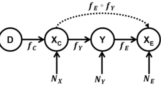
Figure 1: Our setting - CS holds, SSL possible.
et al., 2011). The final target model is then trained on the reweighted/transformed la-belled source sample. Such methods thus focus on the adaptation task which can loosely be thought of as a preprocessing step, but do not involve unlabelled data in the model fitting. When the amount of labelled data is the bottleneck, however, we would like to not only adapt, but also actively improve the supervised source model with unlabelled data.
However, recent work on the independence of causal mechanisms (ICM) (Janzing and Sch¨olkopf, 2010) suggests that such SSL is not possible in a causal learning setting (X →Y) (Sch¨olkopf et al., 2012). Since standard CS implicitly treats all features as causal (Storkey, 2009) (see Section 2.2 for more details), further assumptions are necessary to make SSL work in such a setting. We thus consider an unsupervised CS-adaptation setting for which the amount of labelled data is the main limiting factor, but for which the true causal structure is known. In doing so, we attempt to answer the following question: How can causal knowledge guide a more principled and more effective use of unlabelled data in changing environments?
Specifically, we assume that through prior causal inference, expert knowledge, or back-ground information some features have been identified as effects XE of a target variable Y
while the remaining features represent causes XC. This setting with effect features allows
to combine CS adaptation and SSL, as shown schematically in Fig. 1. Since CS is assumed, it is required that the domain shift (D) does not directly influenceXE (as the v-structure
atXE would otherwise induce a domain dependence ofY, see Fig. 2a).
Two examples of real world scenarios compatible with our idea of prediction from cause and effect features are the following: (i) predicting disease,Y, from risk factors like genetic predisposition or smoking, XC, and symptoms, XE; while we might have (possibly
unla-belled) data from multiple geographical regions or demographic groups leading to different distributions over risk factors (D→XC), we would not necessarily expect this to affect the
behaviour of the disease itself (XC → Y → XE); (ii) predicting the hidden intermediate
state Y of a physical system with inputsXC and outputs XE; again, we might have data
from various experiments with differing input distributions (D → XC), but the laws of
physics or nature (XC →Y →XE) would not be expected to change.
Our approach is a semi-generative model, P(Y, XE|XC, θ), which combines ideas from
invariant prediction (Peters et al., 2016) and SSL, and which arises from the asymmetric roles played by cause and effect features in our setting and under the ICM assumption. This framework leads to a domain invariant model by conditioning on XC and naturally allows
to include unlabelled data in the fitting process by summing or integrating out Y. The latter allows for unsupervised learning of a map from cause to effect features, P(XE|XC),
1.1 Contributions and Organisation of the Paper
In Section 2 we present preliminaries and previous work on which this paper build upon in a common context. Section 3 then forms the theoretical main-part, where we clearly state problem setting and assumptions, and derive our semi-generative modelling framework. In Section 4 we show how our approach can be applied to classification and certain regression problems in practice by describing our experiments on synthetic and real data sets. Em-pirical results of these experiments are presented in Section 5. In Section 6 we critically discuss our results in the context of related work and comment on the general applicability of our approach. Finally, we summarise our findings in Section 7. Some supplementary information is included in the Appendices.
2. Preliminaries & Previous Work
This section covers preliminaries and related work such as the unsupervised domain adapta-tion setting, the covariate shift assumpadapta-tion, causal vs predictive models, the independence of causal mechanisms, the co-training algorithm, and hybrid generative-discriminative models. It may be skipped by a reader familiar with these concepts.
2.1 Unsupervised Domain Adaptation (DA)
In the unsupervised domain adaptation (DA) setting we have access to unlabelled data for the same task but from a different distribution (also called domain in this context). This setting occurs, for example, when training and test sets are not from the same distribution (Quionero-Candela et al., 2009). Formally, we are given a labelled sample SS ={xi, yi}ni=1S
from the source domainP(X, Y|D= 0) and an unlabelled sampleST ={xj}nj=S+nSn+1T from the
target domainP(X, Y|D= 1), whereDis the domain indicator.1 The aim of unsupervised DA is to find a mapping from the shared feature to label space,f :X → Y, which minimises the expected target loss w.r.t. a given loss function L:Y × Y → R. An optimal f is
f∗ ∈argminfEP(·|D=1) h L f(X), Y i = argminf Z P(x, y|D= 1)L f(x), ydxdy. (1)
Since the target distribution P(X, Y|D = 1) is not only unknown but also cannot be estimated due to the lack of target labels, this learning problem is inherently ill posed. Thus, further assumptions about the similarities of source- and target domain are necessary.
2.2 Covariate Shift (CS)
One of the most commonly used assumptions for unsupervised DA is covariate shift (CS). CS states that the difference between domains is only due to a shift in the marginal distri-bution over covariates, or features, while the conditional distridistri-bution of labels given features remains invariant: P(X|D = 0)6= P(X|D = 1), but P(Y|X, D = 0) =P(Y|X, D = 1) =
P(Y|X). This can also be expressed asY ⊥⊥D|X and is depicted as a graphical model in Fig. 2a. Note that the similar graph shown in Fig. 2b does not satisfy the CS assumption due to the v-structure at X, which causes Y to be conditionally dependent of D given X.
(a) CS holds (b) CS does not hold
Figure 2: Two scenarios for domain adaptation: (a) when X causes Y, CS holds since
Y ⊥⊥ D|X; (b) when Y causes X, CS does not hold since the V-structure at X makes Y
dependent on the domainDgivenX. (It is usually assumed, that the domain shift does not directly affect the targetY, for work on such ”target shift” see, e.g., Zhang et al. (2013).)
When changes in environment lead to CS (also termed “domain shift”), it makes sense to consider the edge (D→X) as being truly causal, and such CS can thus be seen as treating all features as causes of Y. We note, however, that other processes such as, for example, sample selection bias can also be seen as instance of CS. For the rest of this work though, we focus on CS in the sense of domain shift and use these words analogously.
As a consequence of CS, the target distribution can be rewritten as
P(X, Y|D= 1) =P(X|D= 1)P(Y|X) =w(X)P(X, Y|D= 0) (2)
where w(X) = PP((XX||DD=1)=0) are so-called importance weights (Shimodaira, 2000; Sugiyama et al., 2007). This implicitly assumes that the target support is contained in the source support; however, different techniques exist to circumvent this requirement, see, e.g., Cortes et al. (2010) for some theoretical analysis of importance weighting.
Since the rightmost expression in Eq. (2) does not involve target labels, it can be used to approximate the expectation in Eq. (1) empirically:
EP(·|D=1) h L f(X), Y i =EP(·|D=0) h w(X)L f(X), Y i ≈ 1 nS nS X i=1 w(xi)L f(xi), yi.
This corresponds to training a model on the importance-weighted source data where the weights can be interpreted as measure of how representative a certain source example is of the target domain (Sugiyama and Kawanabe, 2012).
Another family of approaches for unsupervised DA under CS avoids the use of im-portance weights, and is based instead on finding domain-invariant features in a common subspace (e.g., Gong et al., 2012; Fernando et al., 2013). Generally speaking, these methods first project the inputs to a new spaceX0 via some mapφ:X → X0, and then train a model on these transformed features. φis usually chosen as to minimise the discrepancy between domains: P(φ(X)|D= 0)≈P(φ(X)|D= 1). Note that P(φ(x)|D = 0) =P(φ(x)|D= 1) implies that w(φ(x)) = 1, thus eliminating the need for importance weights when training on fully domain invariant features. Various criteria have been used to measure the dis-crepancy between domains from finite data, such as, e.g., MMD (Pan et al., 2011), HSIC (Yan et al., 2017), mutual information with a domain indicator (Shi and Sha, 2012), or performance of a domain classifier (Ganin et al., 2016).
2.3 Causal Models
Most of the field of machine learning is concerned with predictive models which learn depen-dencies and correlations between variables from training data. Such models are generally
good at making predictions for observational data, i.e., data observed in one environment, and therefore from the same distribution; however, when the underlying system is inter-vened upon—leading to a change in distribution—such predictive models can show arbitrar-ily poor performance. Causal models (Pearl, 2000; Spirtes et al., 2000), on the other hand, by capturingcausation among variables, rather thancorrelation, are able to also predict the behaviour of a system under interventions. They are thus a more general model class than purely predictive models. The drawback of causal models, however, is their need for inter-ventional training data which is often not available; learning cause-effect relationships from purely observational data is difficult in general, and, without further assumptions, some-times even impossible.2 The interested reader is referred to Pearl (2009) for an overview of causal inference techniques, and to Peters et al. (2017) for a more recent account.
Formally, a structural causal model (SCM) (Pearl, 2000) over a set of random variables
{Xi}di=1 is defined by the set of equations
Xi :=fi Pa(Xi), Ni
for i= 1, . . . , d (3)
where Pa(Xi) is the set of causal parents of Xi (i.e., those variables having a direct causal
effect onXi),Niare mutually independent, random noise variables, andfiare deterministic
functions. An illustration of such models in the bivariate case can be found in Fig. 3. Since
Ni are stochastic, the set of Equations (3) induces a distribution P over {Xi}di=1 which
depends on the noise distributions. The corresponding directed acyclic graph (DAG) with
{Xi}di=1 as nodes and Xi → Xj an edge iff. Xi ∈ Pa(Xj) can be thought of as a causal
Bayesian network (Pearl, 1985), i.e., a directed probabilistic graphical model (PGM) in which the direction of edges truly indicates causal influence. The joint distribution factorises over this causal Bayesian network as
P(X1, . . . , Xd) =
d
Y
i=1
P(Xi|Pa(Xi)). (4)
The true power of SCMs over general PGMs is that the former can model interventions, while the latter cannot. An intervention corresponds to setting one of theXito a fixed value
xi, and is denoted using Pearl’s do-operator asdo(Xi =xi). In the SCM framework this can
be modelled by replacing all occurrences of Xi in Equations (3) by the new assignmentxi.
The newly induced distribution (as there is no stochastic contribution fromNi anymore) is
denoted P(·|do(Xi =xi)). It is obtained by replacing the factor P(Xi|Pa(Xi)) in Eq. (4)
withδ(Xi =xi) and all occurrences ofXi ∈Pa(Xj) by xi. We stress here that intervening
on a variable is fundamentally different from conditioning on it: an intervention on Xi
only affects its causal descendants (as these are the only equations in which Xi occurs),
but not its causal ancestors;conditioning onXi, on the other hand, usually affects both its
descendants and ancestors.
While causal models are not necessary for the standard supervised and i.i.d. learning set-ting for which distributions remain unchanged, they can play an important role in analysing and understanding variations to this classical scheme. This is reflected in numerous recent works drawing on ideas from causality to tackle ML problems such as, for example, data
(a) Causal learning, SSL not possible (b) Anticausal learning, SSL possible
Figure 3: Under the ICM assumption, (a) SSL should not be possible ifY :=fY(X, NY),
asP(X) and P(Y|X) are independent in this case; (b) if X := fX(Y, NX) then SSL is, in
principle, possible asP(X) and P(Y|X) may share some information. [Figure reproduced from Sch¨olkopf et al. (2012)]
fusion (Pearl and Bareinboim, 2014; Bareinboim and Pearl, 2016), transfer learning (Magli-acane et al., 2017), multitask learning (Rojas-Carulla et al., 2015), and domain adaptation (Zhang et al., 2015).
2.4 Independence of Causal Mechanisms (ICM)
An assumption with roots in causal modelling which has received attention in recent years is the independence of causal mechanisms (ICM) which was inspired by Lemeire and Dirkx (2006) and formalised in terms of algorithmic complexity by Janzing and Sch¨olkopf (2010). At its heart is the assumption that the fi in Equations (3) are mutually independent, so
that the conditionalsP(Xi|Pa(Xi)), orcausal mechanisms, on the RHS of Eq. (4) represent
”autonomous modules that do not inform or influence each other” (Parascandolo et al., 2017).
The implications of this assumption for different learning settings have been discussed by Sch¨olkopf et al. (2012), which is one of the main inspirations for the current work. In particular, the authors argue that since SSL relies on linking P(X) and P(Y|X) it should not be possible in the causal direction (Fig. 3a) asP(X) andP(Y|X) represent independent causal mechanisms in this case. In an ”anticausal” learning setting (Fig. 3b), on the other hand, when the causal mechanisms are P(Y) andP(X|Y), P(X) andP(Y|X) might still exhibit some dependence so that SSL is, in principal, possible. Empirical evidence supports the validity of this argument (Sch¨olkopf et al., 2012).
2.5 Other Previous Work
In addition to those referred to already in the previous sections, we review similarities and differences to some other previous work below.
Co-Training: One of the earlier and most influential works on combining labelled and
unlabelled data is the ”Co-Training” algorithm by Blum and Mitchell (1998). Motivated by boosting performance of a web-page classifier using a large unlabelled sample the authors assume that: (i) the feature set can be split into two disjoint views,X= (X1, X2), which are
conditionally independent givenY; and (ii) each view is sufficient for learning the task given enough data. They then train a weak classifier on each view, and use these to iteratively label unlabelled examples and add them to the training set. While there are some clear parallels to our approach, e.g., assumption (i) above also holds in our setting, we do not
assume that each view (XC and XE in our case) is sufficient on its own (assumption (ii)
above). More importantly, our approach does not rely on assigning labels to unlabelled data and is therefore not part of the family of self-learning approaches to SSL of which co-training is a member.
Hybrid Generative-Discriminative Models: Since Ng and Jordan (2002) shed light
on some of the advantages and disadvantages of discriminative vs. generative models, some works have attempted to combine these two approaches for SSL. Multi-conditional learning (McCallum et al., 2006) considers objective functions like P(Y|X)αP(X)β and has been
successfully applied to SSL (Druck et al., 2007). An example of combining SVM and naive Bayes for SSL can be found in Jiang et al. (2013). The idea of combining supervised and unsupervised components in the objective function is also reflected in our approach. However, the above-mentioned works train both a generative and a discriminative model using the former for unlabelled and the latter for labelled data; on the other hand, we only trainone model which is neither fully generative nor fully discriminative, and which can be used to include both unlabelled and labelled data.
Learning with Cause and Effect Features: To the best of our knowledge no
pre-vious works explicitly consider learning from both cause and effect features. The closest may be that of Kang and Tian (2006) where—even though not in a causal context—they consider two sets of features X1 and X2 on either side of Y. The resulting likelihood P(Y|X1)P(X2|Y) is similar to ours, but is not used in combination with unlabelled data.
3. Semi-Generative Modelling
In this Section we explicitly state our assumptions, use them to derive our semi-generative framework, and show how it gives rise to a modelling approach which naturally allows for including unlabelled data, while remaining robust to distribution shifts over causal features.
3.1 Assumptions
We consider the unsupervised domain adaptation problem of predicting the outcome of a random variable Y in a target domain (D = 1) from an observation of a set of random variables, or features, X. We assume that the set of features can be partitioned into two disjoint, non-empty sets: X =XC∪XE and XC 6=∅6=XE. As training data we are given
a labelled, typically small set of observations SS ={(xiC, yi, xiE)}ni=1S from a source domain
(D= 0) and an unlabelled, typically large set ob observationsST ={(xjC, x j E)}
nS+nT
j=nS+1 from
a target domain (D= 1). Moreover, we make the following main assumption.
Assumption 1 (Known Causal Structure & ICM) The relationship between the
vari-ables XC, Y,XE and the domain indicatorD is accurately captured by the following SCM:
XC :=fC(D, NC)
Y :=fY(XC, NY)
XE :=fE(Y, NE)
(5)
whereNC,NY, andNE are mutually-independent random noise variables, and the functions
This SCM is shown schematically in Fig. 4. The (unknown) distributions over noise vari-ables together with Equations (5) induce a distribution over (XC, Y, XE) which depends
on D: P(XC, Y, XE|D). We will refer to the two distributions P(XC, Y, XE|D = 0) and
P(XC, Y, XE|D= 1) as source and target distributions, or domains, respectively.3
3.2 Analysis
From Eq. (4) and Assumption 1 it follows that the distributionP factorises as
P(XC, Y, XE|D) =P(XC|D)P(Y|XC)P(XE|Y). (6)
where the factors on the RHS correspond to the three independent causal mechanisms. This factorisation can be used to show that the CS assumption is satisfied in our setting (as intended by construction).
Proposition 1 CS holds for the setting described by Assumption 1.
Proof By the factorisation of P given in Eq. (6), it follows that:
P(Y|XC, XE, D) = P(XC, Y, XE|D) P(XC, XE|D) = P(Y, XE|XC)P(XC|D) P(XE|XC)P(XC|D) = P(Y, XE|XC) P(XE|XC) .
The last equality shows that the conditional distribution does not depend on the domainD.
In fact, we can make a stronger statement than Proposition 1. This is due to the assumed chain-like problem structure which results in a direct shift only in the distribution over causes, P(XC|D). Whereas this change in distribution is propagated through the
mecha-nisms P(Y|XC) and P(XE|Y) thereby also affectingY and XE, the only shift that needs
to be corrected for is that inXC. This follows directly from the factorisation (6):
P(XC, Y, XE|D= 1) =w(XC)P(XC, Y, XE|D= 0) (7)
wherew(XC) =PP((XXCC||DD=1)=0) are importance weights (Shimodaira, 2000). Hence, conditioning
on XC is sufficient to obtain domain-invariance.
Eq. (7) also reveals a first side-benefit of identifying some features as effects in a CS setting: training a model on reweighted source data only requires estimation of the distri-bution over causes, but not over effects. Since the correct weights are generally not known, estimating such ratios of (potentially high-dimensional) distributions from limited data is often a challenge a practice. Performing this estimation over a lower-dimensional space could thus be advantageous.
The focus of our work, however, lies on actively improving the source model from unla-belled data, rather than on the adaptation task. By improvement here we refer to obtaining a better estimate of the conditional distributionP(Y|XC, XE) and ultimately a lower error
rate on an unseen test set drawn from the target domain. According to the ICM assumption, such semi-supervised learning is not possible in the causal direction but might work in the anticausal direction (see Fig. 3) (Sch¨olkopf et al., 2012). This has the following implications for our setting:
3. Note that even though we focus on the caseD∈ {0,1}here, it should be simple to include additional labelled or unlabelled data from different sources as in domain generalisation.
Figure 4: A schematic illustration of the assumed causal problem structure. The dashed arrow illustrates the main idea of our approach, namely learning a map from cause to effect features from unlabelled data and using it as a soft model constraint.
• The distribution over causal features does not share any information with the condi-tional distribution of Y. A better estimate of P(XC|D) obtainable from unlabelled
data will therefore not help to improve our estimate of the conditional, and so ex-plicitly modelling the cause distribution unnecessarily introduces model complexity without apparent benefits.
• P(Y) and P(XE|Y) are independent mechanisms, but P(XE) and P(Y|XE) may
contain shared information. We can therefore hope to improve our estimate of the conditional via a better estimate ofP(XE) from the unlabelled sample. This suggests
explicitly modelling the distribution over effects in our case.
One way to convince oneself of the above is from the domain invariant form of the condi-tional, P(Y,XE|XC)
P(XE|XC) , where XC only appears as a variable which we condition on, whereas
XE appears explicitly. We note here that while it is also possible to write the conditional
P(Y|XC, XE) differently, only conditioning onXC leads to a domain invariant form. Such
invariance is required as those terms involving Y can only be estimated from the source domain, while we wish to make predictions for the target domain.
Another way to understand the different roles played by cause and effect features is from the SCM (5) in Assumption 1. Even if one could perfectly learn the data generating process for the causal features, XC :=fX(D, NC), this does not reveal anything aboutY.
The generating process for the effects,XE :=fE(Y, NE), on the other hand, clearly depends
on Y. In particular, when Y is unknown but XC is known—as is the case for the large
unlabelled sample from the target domain—we can substitute forY to obtain
XE :=fE(Y, NE) =fE fY(XC, NY), NE
. (8)
Equation (8) above demonstrates our main idea: by learning a (noisy) map from causes to effects from unlabelled data we hope to improve our estimates of the functionsfY andfE,
and thereby also our predictive model. Such a map can be viewed as a noisy composition of functions, fE◦fY, as indicated by the dashed arrow in Fig. 4.
In terms of the distribution P this idea corresponds to improving our estimate of
P(XE|XC). Factorising the distribution from which the unlabelled sample is drawn as
helps to illustrate the point of our approach. Whereas CS adaptation by importance weight-ing would only use the first term on the RHS of Eq. (9) thereby disregardweight-ing half the un-labelled sample, our approach will make full use of all unun-labelled data by using the second term for semi-supervised learning.
3.3 Modelling Approach
The previous analysis of the asymmetric roles played by cause and effect features suggests using a model of the form P(Y, XE|XC, θ). We refer to this modelling framework as
semi-generative, as it can be seen as an intermediate between a fully semi-generative,P(XC, Y, XE|θ),
and a fully discriminative, P(Y|XC, XE, θ), framework. As opposed to a fully generative
model, the semi-generative model is domain invariant due to conditioning on XC. At the
same time, the semi-generative framework also allows including unlabelled data by summing (ifY is discrete) or integrating (if Y is continuous) out Y,
P(XE|XC, θ) =
XZ
y∈Y
P(Y =y, XE|XC, θ) [dy] (10)
which is not possible for fully discriminative models which condition on all features. For our setting, a semi-generative framework thus combines the best from both worlds: domain invariance and the possibility to include unlabelled data in the fitting process.
As it does not depend on labels, we will also refer to Eq. (10) as the unsupervised model. It is clear that we can always obtain the unsupervised model for classification tasks, while for regression we are restricted to special types of submodels for which the integral can be computed analytically. When other models are desired, approximating the integral is an option, but this is left for future work.
Moreover, the semi-generative formulation has another advantage in our setting: it factorises into the two independent mechanisms
P(Y, XE|XC, θ) =P(Y|XC, θY)P(XE|Y, θE) (11)
where θ= (θY, θE) are the parameters of the two submodels. Note that this can also help
avoid problems with missing data. E.g., if xiC is missing for some i, the pair (yi, xiE) can still be used to train P(XE|Y, θE).
With our model P(Y, XE|XC, θ), a way to include unlabelled data via Eq. (10), and
the factorisation into two submodels given by Eq. (11) we are now ready to give a high-level summary of our approach:
1. Train two supervised submodels, P(Y|XC, θY) and P(XE|Y, θE), on labelled pairs
(xiC, yi) and (yi, xiE), such that the corresponding unsupervised model (10) ’agrees well’ with the unlabelled cause-effect pairs (xjC, xjE).
2. Construct the probabilistic conditional from P(Y|XC, θY) andP(XE|Y, θE) as:
P(Y|XC, XE, θ) =
P(Y|XC, θY)P(XE|Y, θE)
PR
y∈YP(Y =y|XC, θY)P(XE|Y =y, θE) [dy]
(12)
A likelihood-based version of the above is described in detail in the next section and sum-marised for classification in Algorithms 1 and 2 in Appendix B.
3.4 (Log-)Likelihoods
The average supervised source likelihood,P(Y, XE|XC, θ), of our model given the observed
labelled data is given by:
LS(θ) =L(θ|SS) = nS Y i=1 P(yi, xiE|xiC, θ) 1 nS = nS Y i=1 P(yi|xiC, θY) 1 nSP(xi E|yi, θE) 1 nS.
We consider average (log-)likelihoods in order to be able to compare models trained on different amounts of data; such averaging does, of course, not affect the resulting parameter MLEs. The corresponding average log-likelihood`is given by
`S(θ) = 1 nS nS X i=1 logP(yi|xiC, θY) + logP(xiE|yi, θE) (13)
and can be maximised w.r.t. θY andθE separately. Closed form MLEs are thus often
avail-able for simple enough models. The same holds true for LW S and `W S which additionally
importance-reweigh term iinLS and `S, respectively, byw(xiC) (Shimodaira, 2000).
`W S = 1 nS nS X i=1 w(xiC) logP(yi|xiC, θY) + logP(xiE|yi, θE) (14)
Note that importance weights arise from an empirical source approximation to the expected target loss and are thus not subject to logarithms.
Our approach suggests additionally including unlabelled data via the average unsuper-vised target likelihood, P(XE|XC, θ):
LT(θ) =L(θ|ST) = nS+nT Y j=nS+1 P(xjE|xjC, θ) 1 nT = nS+nT Y j=nS+1 XZ y∈Y P(y|xjC, θY)P(xjE|y, θE)[dy] 1 nT
where the last equality follows from Equations (10) and (11). The corresponding target log-likelihood is `T(θ) = 1 nT nS+nT X j=nS+1 log X Z y∈Y P(y|xjC, θY)P(xjE|y, θE)[dy] .
We propose to combine labelled and unlabelled data in the pooled likelihood as
LP(θ) =L(θ|SS, ST) =LS(θ)λLT(θ)1−λ
with corresponding log-likelihood
`P(θ) =λ `S(θ) + (1−λ)`T(θ) (15)
where the hyperparameter λ ∈ (0,1) interpolates between the average source- and target likelihoods and can be chosen depending on nS and nT. E.g., λr = nSn+SnT gives equal
weight to all observations and is therefore a natural choice, while changing this ratio leads to different weights for labelled and unlabelled data.
4. Experiments
In order to analyse our approach, we perform some regression and classification experiments on synthetic data sets. Moreover, we apply our semi-generative approach to a real world protein-signalling network data set (Sachs et al., 2005) to investigate its applicability in practice. For classification, we consider maximum likelihood and Bayesian approaches under both correct parametrisation and model misspecification to identify potential strengths and weaknesses in different settings. This Section contains the necessary experimental details to reproduce our results, and can be used as a guide to applying our semi-generative modelling approach for new classification and regression problems.
4.1 Estimators
Since our method requires making certain assumptions about the causal structure, and in order to make comparisons as fair as possible, we study our approach relative to versions of the source-only baseline and the importance-weighting technique, which take the known causal structure into account. In particular, we compare:
• θˆS: training a model on the labelled source data only. It ignores the unlabelled data
and thus corresponds to no adaptation, but takes causal knowledge into account.
• θˆW S: training a model on the importance-weighted source data. It thus uses only the
“XC-part” of the unlabelled sample and ignores the “XE-part”, see Eq. (7). In our
experiments we use known weights; however, in practice these would also have to be estimated from data.
• θˆP (our proposed estimator): training a model on the pooled data set combining
unweighted labelled and unlabelled data via λas explained in Section 3.4. (A second pooled estimator ˆθW P using weighted, instead of unweighted, labelled data was
ini-tially considered, but was then dropped for clarity of results as it suffered from the same problems as ˆθW S related to reweighting.)
• θˆLR: training a standard linear/logistic regression model on the joint feature set
(XC, XE), i.e., ignoring the known causal structure. Where applicable, we report the
performance ofθLR for comparison.
Moreover, we compare our method to some state-of-the-art feature-transformation based approaches to unsupervised DA such as transfer component analysis (TCA, Pan et al., 2011), maximum independence domain adaptation (MIDA, Yan et al., 2017), subspace alignment (SA Fernando et al., 2013), geodesic flow kernel (GFK Gong et al., 2012), and information theoretical learning (ITL, Shi and Sha, 2012, for classification only). As would be the case without any knowledge of the causal structure, we apply these methods on the pooled data set (including source labels where applicable), and then train a linear/logistic regression model (as for ˆθLR) on the new set of transformed features. We use the implementation
and default parameters provided in the MATLAB domain adaptation toolbox by Yan, Ke (2016).
4.2 Model Fitting: Maximum Likelihood and Bayesian Approaches
For model fitting by maximum likelihood (ML), we minimize the negative log-likelihood (NLL) which acts as a proxy for the 0-1 loss in the case of classification and root mean squared error (RMSE) in the case of regression. The ML estimates ˆθS, ˆθW S, and ˆθP are
thus found by maximising `S (13), `W S (14), and `P (15), respectively. We use
analyti-cal solutions where available and gradient descent to minimise the negative log-likelihoods otherwise.
For a Bayesian approach, we place a rather flat (i.e., with large σ) normal prior π on
θ, so as to not include much prior knowledge on how the data is generated. We can then compute the log-posterior distribution up to additive constants:
logP(θP |SS, ST) = logπ(θ) + (nS+nT)`P(θ) + const., (16)
In order to make predictions for new data (xnewC , xnewE ), we estimate the required integral using a Monte Carlo approximation:
P(Y =y|xnewC , xnewE ) = Z θ P(Y =y|xnewC , xnewE , θ)P(θ|SS, ST) dθ ≈ 1 K K X k=1 P(Y =y|xCnew, xnewE , θ(k))
whereθ(k) are samples from the posterior distribution. We use a Metropolis-Hastings algo-rithm (Metropolis et al., 1953; Hastings, 1970) with a multivariate normal proposal distribu-tion to sample from the corresponding unnormalised log-posterior distribudistribu-tion (16). In our experiments we use a step size of 0.1 and generate 10 randomly-initialised Markov chains of length 1100, in order to avoid the sampler getting stuck in local maxima of spiky, multi-modal posteriors. Discarding the first 100 samples from each chain as burn-in, this leaves 10,000 samples for prediction. (Of course, more elaborate sampling schemes are possible.)
4.3 Synthetic Classification Experiments
For the classification experiments, we focus on binary classification. However, it is straight-forward to extend our method to multi-class classification as well. To generate synthetic classification data sets with a simple linear decision boundary, but which are still some-what challenging due to class-overlap, and which comply with our assumptions, we use the following SCM: XC := ( µC +C if D= 0, −µC+C if D= 1, where C ∼ N(0, σC2) Y := ( 1 if Y ≤sigm s(XC−m) , 0 if Y >sigm s(XC−m) , where Y ∼U(0,1) XE := ( µ0+σ0E if Y = 0, µ1+σ1E if Y = 1, where E ∼ N(0,1) (17)
with all noise variables i mutually independent, and where sigm is the logistic sigmoid
function, sigm(x) = (1 +e−x)−1. This induces the distributions
Y |(XC =xC)∼Bernoulli sigm s(xC−m) XE|(Y =y)∼ ( N(µ0, σ02) if y = 0 N(µ1, σ12) if y = 1 . (18)
From (18) we can compute the unsupervised model (Eq. (10)) by summing outY:
P(XE =xE|XC =xC, θ) = 1 X y=0 P(XE =xE|Y =y, θE)P(Y =y|XC =xC, θC) = 1 +e−s(xC−m)−1φ(x E|µ0, σ02)e−s(xC−m)+φ(xE|µ1, σ12) where φ(x|µ, σ2) = (2πσ2)−12e− (x−µ)2
2σ2 is the pdf of a normally distributed random variable
with mean µand standard deviationσ. Substituting this expression in`P and maximising
w.r.t. θ yields our estimator ˆθP. We can then classify new examples using the probabilistic
conditional P(Y|XC, XE,θˆP) from Eq. (12).
To reduce the number of unknown parameters fitted from very little data and to make it comparable to the three parameters of a standard logistic regression model for our setting, we assume all σ2 and the sigmoid shape parameter s to be known and equal to one in our simulations. At each iteration, we then draw a new set of parameters µC, θY = m,
θE = (µ0, µ1), where µC, µ1 ∼ U(0,1), m ∼ U(−1,1), and µ0 ∼ U(−1,0). Next, we
generate a synthetic data set by drawing nS labelled and nT unlabelled samples from the
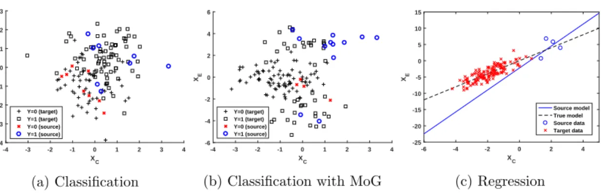
source- and target domains, respectively, according to Eq. (17). One such classification data set is shown examplary in Fig. 5a. For ˆθS and ˆθW S we use the closed-form weighted least
squares solutions as MLEs for µ0 and µ1, whereas all other estimates need to be found by
gradient descent due to the non-linearity of the sigmoid function.
Furthermore, we perform some additional classification experiments to investigate the behaviour of our approach under model-misspecification. To achieve this, we fit exactly the same model as before (i.e., a linear decision boundary) while changing one of the normal distributions into a mixture of Gaussians (MoG). Specifically, we set µ0 = 0 and µ1= 3 to
ensure strong non-linearity and then draw the class-1 effects according to
XE|(Y = 1)∼
1
2N(−µ1,1) + 1
2N(µ1,1).
An example of such a classification data set generated with a MoG is shown in Fig. 5b.
4.4 Synthetic Regression Experiments
For our synthetic regression experiments, we focus on a linear setting with Gaussian noise. Albeit a very simple model, linear regression is still widely used on small data sets. Morevoer, it has the advantage of high interpretability of parameter estimates and is thus still a pop-ular choice, e.g., in social sciences. Finally, the integral in Eq. (10) required for continuous
-4 -3 -2 -1 0 1 2 3 4 XC -4 -3 -2 -1 0 1 2 3 XE Y=0 (target) Y=1 (target) Y=0 (source) Y=1 (source) (a) Classification -4 -3 -2 -1 0 1 2 3 4 XC -6 -4 -2 0 2 4 6 XE Y=0 (target) Y=1 (target) Y=0 (source) Y=1 (source)
(b) Classification with MoG
-6 -4 -2 0 2 4 XC -25 -20 -15 -10 -5 0 5 10 15 XE Source model True model Source data Target data (c) Regression
Figure 5: Our synthetic data sets. Shown are classification data under normal conditions in (a), and with a mixture of Gaussians forXE|Y = 1 as used for the model-misspecification
experiments in (b). For both, target labels are not available during training. (c) shows the regression data along with the true model and the corresponding fit from source data.
models). We thus generate synthetic regression data according to the following linear SCM:
XC := ( α+C if D= 0, −α+C if D= 1, where C ∼ N(0, σ2C) Y :=a+bXC+Y, where Y ∼ N(0, σ2Y) XE :=c+dY +E, where E ∼ N(0, σE2) (19)
with all noise variables i mutually independent. This induces the distributions
Y |(XC =xC)∼ N(a+bxC, σY2)
XE|(Y =y)∼ N(c+dy, σE2).
(20)
Substituting for Y in the last line of Eq. (19), we obtain
XE =c+ad+bdXC +dY +E.
From a standard result about the sum of two normally distributed random variables applied todY andE, it then follows that
XE|(XC =xC)∼ N(c+ad+bdxC, d2σ2Y +σE2) (21)
which allows us to compute and maximise`P to obtain our proposed estimator ˆθP. In order
to predict in the regression setting, we also need to provide a closed form solution to the argmax of the probabilistic conditional P(Y|XC, XE,θˆP):
Proposition 2 Given the regression model in Eq. (19) and a parameter estimate θ, the
most likely outcome for a new observation (x∗C, x∗E) is given by
y∗= σ 2 E(a+bx ∗ C) +d2σ2Y( x∗E−c d ) σ2 E+d2σ2Y .
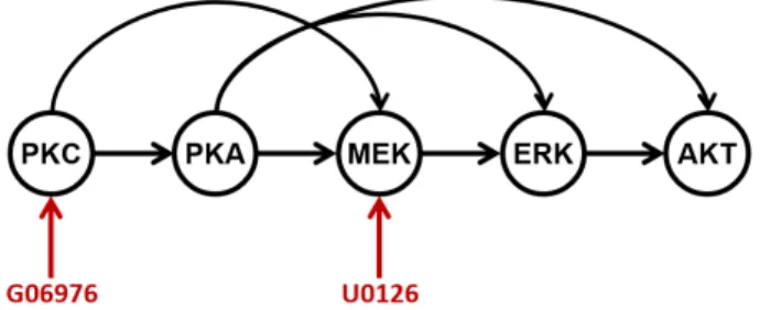
Figure 6: Shown is the subset of variables from the protein-signalling network which we used for our experiments. Arcs indicate causal links, and shown in red are interventions on PKC and MEK via the substances G06976 and U0126, respectively. For more details the reader is referred to the original paper (Sachs et al., 2005).
The predictiony∗ in Proposition 2 can be seen as a weighted average of the two submodels’ predictions, where inverse weights correspond to each model’s uncertainty.
Simulations are then performed as follows: Firstly, all σ2s are assumed to be known and equal to one, while the remaining parametersα,θY = (a, b), andθE = (c, d) are drawn
anew from a hyperprior at each iteration, where α ∼ U(0,2) and a, b, c, d ∼ U(−2,2). Next, we generate a synthetic data set by drawing nS labelled and nT unlabelled samples
from the source- and target domains, respectively, according to Eq. (19). We then compute the different estimators using the analytical (weighted) least squares solutions forθS,θW S,
and θLR, whereas θP is found using gradient descent, as the unsupervised target model is
non-linear in the parameters, see Eq. (21).
4.5 Real-Data Regression Experiments
As a real-world example we use the “Causal Protein-Signalling Network” data set published by Sachs et al. (2005). It contains single-cell measurements of 11 phospho-proteins and phospho-lipids under 14 different experimental conditions, as well as—importantly for our method—the corresponding causal Bayesian network inferred from this interventional data. In our experiments, we focus on a subset of variables which is shown in Fig. 6. This subset was selected to be most compatible with our assumptions.
We extract two data sets of different difficulty from this subset of variables: D1, which
corresponds to MEK (XC)→ ERK (Y)→AKT (XE), and D2, which coresponds to PKC
(XC) → PKA (Y) → AKT (XE). For both, source data consists of measurements under
normal conditions and target data is obtained by intervening on MEK in the case ofD1 and
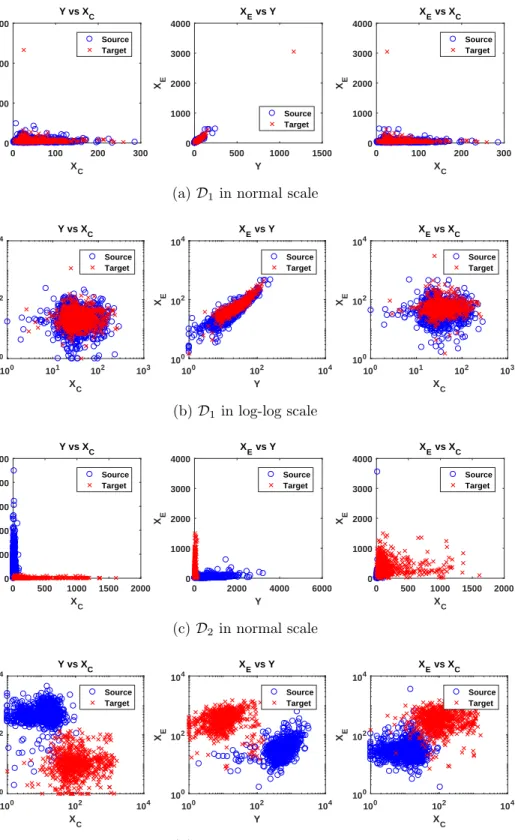
on PKC in the case of D2. The two real-world data sets are shown in normal and log-log
scale in Fig. 7. As can be seen, D1 shows a high similarity between domains, whereas D2
appears to be more challenging due to the high domain discrepancy.
As is often the case with biological data, features span multiple orders of magnitude and are thus more easily visualised in log-space. Moreover, all relationships between variables, i.e., protein-protein interactions, seem to be reasonably-well approximated by power laws (Y =AXb) which is also often true for natural systems. In our case, we can think of protein
X as either facilitating or inhibiting expression of proteinY, roughly resulting in an either linear or inverse relationship, respectively. For these reasons, we decide to first transform
the data by taking logarithms (which is not a problem as all features, being protein counts, are ≥1). We then fit a linear model in log-space (logY =a+blogX) which corresponds to fitting a power law in the original space.
We then perform simulations on the real data sets as follows. At each iteration, we draw a fixed number nS of labelled observations from the source domain, and reserve 200
observations from the target domain as a test set. From the remaining target data, we
draw nT = 2,4, ...,512 additional observations as unlabelled training data. We then fit a
linear model as described in the previous Section for synthetic regression experiments, with the difference that we also treat σ2Y and σE2 as unknown. The model parameters are thus
θY = (a, b, σ2Y), and θE = (c, d, σE2), with mechanisms as in Eq. (20), the unsupervised
model as in Eq. (21), and predictions are made according to Proposition 2.
Finally, to investigate how background knowledge can aid our approach in real world applications, we also perform simulations on D2 under the constraintb, d≤0 , i.e., fitting lines with negative slope. This constraint captures that both PKC → PKA and PKA →
AKT are inverse relationships which might be known from domain expertise. To accommo-date parameter constraints in our optimisation routine, we maximise over β, δ, sY, sE ∈R
setting b=−eβ,d=−eδ,σY2 =esY, and σ2
E =esE.
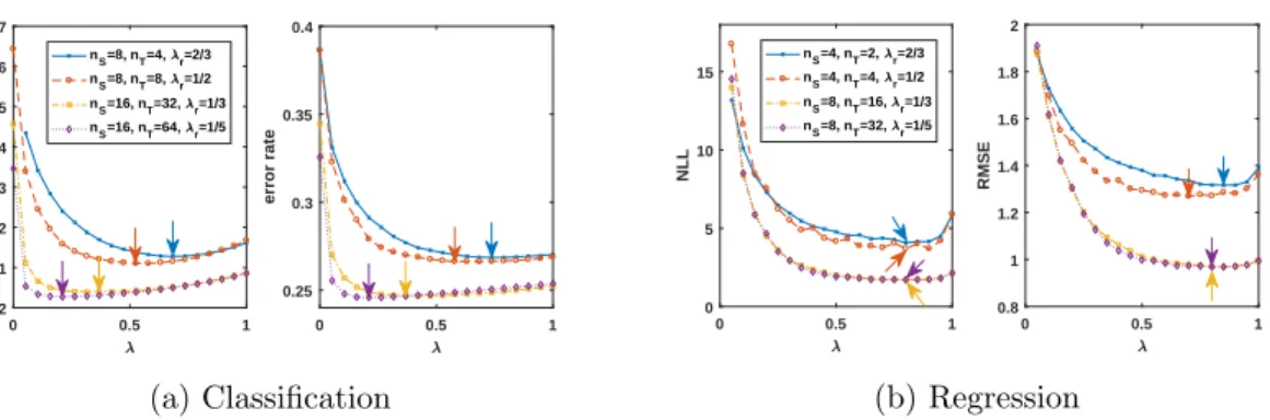
4.6 Choosing λ
To choose the hyperparameter λ ∈ (0,1) we perform a grid search, considering different combinations of nS and nT. This is done for synthetic classification and regression data
generated as described in the previous section with a fixed choice of parameters. The results are shown in Fig. 8. For classification, we find thatλr(nS, nT) = nnS
S+nT giving equal weight
to all observations (i.e., more weight to the unsupervised model asnT is increased) appears
to be a good choice across different settings, see Fig. 8a.
In contrast, for regression a good choice of λ does not seem to depend on nT. Rather
than weighting all observations equally, values of λ giving large weight to the supervised model appear to be preferred for regression. Following the results of Fig. 8b, we thus choose a constant λ= 0.8 for our regression experiments.
Finally, we note that as the amount of labelled data is increased, the unsupervised model seems to become obsolete for simple linear regression problems. One could thus also consider choosingλ(nS) to approach 1 for largenS: e.g., a choice likeλ(nS) = 1−n1S could
be reasonable.
4.7 Evaluation
For both classification and regression experiments on synthetic data, we draw a test set of size 103 from the target domain and use it to evaluate the different estimators. The simulation steps described in Sections 4.3 and 4.4 are then repeated niter ≥ 103 times,
which each iteration corresponding to a different set of model parameters. This yields an average performance over many different classification/regression problems, thus avoiding overfitting to any particular parameter configuration and increasing the robustness of our findings.
We report both negative log-likelihood (NLL) and actual loss (RMSE/error rate) test-set averages, as recommended by Loog and Jensen (2015), for the following reason: while
0 100 200 300 XC 0 500 1000 1500 Y Y vs X C Source Target 0 500 1000 1500 Y 0 1000 2000 3000 4000 XE X E vs Y Source Target 0 100 200 300 XC 0 1000 2000 3000 4000 XE X E vs XC Source Target
(a)D1 in normal scale
100 101 102 103 XC 100 102 104 Y Y vs XC Source Target 100 102 104 Y 100 102 104 XE XE vs Y Source Target 100 101 102 103 XC 100 102 104 XE XE vs XC Source Target (b)D1 in log-log scale 0 500 1000 1500 2000 XC 0 1000 2000 3000 4000 5000 Y Y vs XC Source Target 0 2000 4000 6000 Y 0 1000 2000 3000 4000 XE XE vs Y Source Target 0 500 1000 1500 2000 XC 0 1000 2000 3000 4000 XE XE vs XC Source Target (c) D2 in normal scale 100 102 104 XC 100 102 104 Y Y vs XC Source Target 100 102 104 Y 100 102 104 XE XE vs Y Source Target 100 102 104 XC 100 102 104 XE XE vs XC Source Target (d)D2 in log-log scale
Figure 7: Shown are the two real-world data sets used in our experiments. D1 corresponds
to MEK(XC) → ERK(Y) → AKT(XE), and D2 to PKC(XC) → PKA(Y) → AKT(XE).
0 0.5 1 0.25 0.3 0.35 0.4 error rate 0 0.5 1 2 2.1 2.2 2.3 2.4 2.5 2.6 2.7 NLL nS=8, nT=4, r=2/3 nS=8, nT=8, r=1/2 nS=16, nT=32, r=1/3 nS=16, nT=64, r=1/5 (a) Classification 0 0.5 1 0 5 10 15 NLL nS=4, nT=2, r=2/3 nS=4, nT=4, r=1/2 nS=8, nT=16, r=1/3 nS=8, nT=32, r=1/5 0 0.5 1 0.8 1 1.2 1.4 1.6 1.8 2 RMSE (b) Regression
Figure 8: Tuning the hyperparameterλ- Shown are negative log-likelihood and RMSE/error rate against λ∈(0,1) for different combinations of nS and nT (see legends); arrows mark
the minima of each curve. All results are test set averages over 104 runs.
we are often mainly interested in a small RMSE or 0-1 loss, optimisation of this quantity generally suffers from non-convexity-related issues so that our model is instead trained to minimise a surrogate loss. In our case, this surrogate loss is the semi-generative, negative log-likelihood: −logP(Y, XE|XC, θ) =−logP(Y|XC, θY)−logP(XE|Y, θE).
5. Results
Here we present the results of our experiments described in the previous section. Unless explicitly stated, all curves show test-set averages over 104 simulations usingλ= nS
nS+nT for
classification andλ= 0.8 for regression. As we report averages over many different synthetic data sets, variances can be quite large, and so we omit error bars for clarity. However, applying a paired t-test to, e.g., the results from Fig. 9 indicates statistical significance
withp <0.05 (and much smaller p-values for largenT), and similar results can be expected
for the other plots, provided that sufficiently many simulations are performed.
Throughout, we mainly consider two settings: one with a very small amount of labelled data (nS = 8 for classification,nS = 4 for regression) and the other with a medium amount
of labelled data (nS = 64 for classification,nS = 16 for regression). We then investigate the
relative performance of our approach as the amount of unlabelled data (nT) is increased.
This reflects our aim of improving the source model with unlabelled data, when labelled training data is very scarce.
Note that whilenS = 8 (or even 4 for regression) may seem like an unrealistically small
amount of labelled data, this always has to be considered relative to the dimensionality. As our synthetic (and real) data sets have two-dimensional feature space, this corresponds to
≈3 (or 2 for regression) observations per dimension. Due to the curse of dimensionality (i.e., the number of data required increase exponentially with the dimensionality of the problem) our setting of 2 or 3 observations per dimension, is thus quite realistic for high-dimensional problems.
100 101 102 103 104 105 n T 2 2.05 2.1 2.15 2.2 2.25 2.3 NLL 100 101 102 103 104 105 n T 0.22 0.24 0.26 0.28 0.3 0.32 error rate P S WS LR (a)nS = 8 100 101 102 103 104 105 nT 1.98 2 2.02 2.04 NLL 100 101 102 103 104 105 nT 0.22 0.225 0.23 0.235 0.24 0.245 0.25 error rate (b)nS = 64 100 101 102 103 104 nT 4.4 4.6 4.8 5 5.2 5.4 NLL 100 101 102 103 104 nT 0.3 0.32 0.34 0.36 error rate P S WS LR (c) nS= 8 (misspecified) 100 101 102 103 104 nT 4 4.5 5 NLL 100 101 102 103 104 nT 0.3 0.32 0.34 0.36 0.38 error rate (d)nS = 64 (misspecified)
Figure 9: Classification results using maximum likelihood parameter estimates under correctly-specified (top row) and misspecified models (bottom row).
5.1 Synthetic Classification Results
Using our synthetic classification data set, we perform maximum likelihood estimation and Bayesian modelling under both correctly specified and misspecified models. Moreover, in the case of a correct model and fitting by maximum likelihood, we also compare our estimators with different feature-transformation methods followed by fitting a logistic regression model. Results of using maximum likelihood estimation are shown in Fig. 9. For a correct model (top row), the curves of NLL and error rate look very similar and follow the same behaviour (despite the NLL curve being slightly smoother). For both small and medium
nS, the source-only baselineθS performs better than the importance-weighted model θW S.
Our pooled-data estimatorθP performs best, with error and NLL decreasing monotonically
withnT. This decrease is much more pronounced fornS = 8 with an absolute improvement
of 4% in error rate for large nT, compared to θS. With nS = 64 labelled examples, on the
other hand, this improvement in error rate drops to only a little over 0.5%.
Under model-misspecification (bottom row), the observed behaviour is very different as the curves of NLL and error rate are no longer aligned. Specifically, while NLL is mono-tonically increasing with nT, error rate increases initially, then peaks for an intermediate
value of nT, and eventually decreases again reaching the lowest value among all estimators
100 101 102 103 104 nT 2 2.2 2.4 2.6 NLL P S WS 100 101 102 103 104 nT 0.22 0.24 0.26 0.28 0.3 0.32 error rate (a)nS = 8 100 101 102 103 104 n T 1.98 2 2.02 2.04 2.06 2.08 NLL 100 101 102 103 104 n T 0.22 0.225 0.23 0.235 0.24 0.245 0.25 error rate (b)nS = 64 100 101 102 103 104 nT 4.6 4.8 5 5.2 5.4 NLL P S WS 100 101 102 103 104 nT 0.29 0.3 0.31 0.32 0.33 0.34 0.35 error rate (c) nS= 8 (misspecified) 100 101 102 103 104 n T 4 4.5 5 NLL 100 101 102 103 104 n T 0.3 0.32 0.34 0.36 error rate (d)nS = 64 (misspecified)
Figure 10: Classification results using a Bayesian approach for correctly-specified (top row) and misspecified (bottom row) models. Shown are averages over 103 simulations.
attained over the range of nT considered is lower than for nS = 64. In the case of the
latter, the structure-agnostic logistic regression model,θLR, yields the lowest error rate for
nT <5×10³. θS and θW S show similar performance in terms of error rate both for small
and medium nS, and yield the lowest error fornS = 8 andnT <4×10² beyond which θP
is to be preferred.
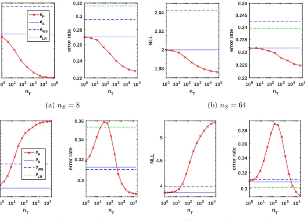
Bayesian results for the same experiments as in Fig. 9 are shown in Fig. 10. While the overall behaviour is very similar between ML- and Bayesian approaches, mainly two differences can be observed. Firstly, using a Bayesian approach under a correct model (top row), we find that some learning curves are no longer strictly decreasing, but instead reach a minimum and increase again for very large nT. For both NLL curves this minimum
occurs at about nT ≈103. Moreover, for nS= 64, the later increase in NLL is much more
pronounced and even error rate reaches a minimum before increasing again, which is not the case for nS= 8.
The second observed difference using a Bayesian as opposed to a maximum likelihood approach is that the former seems to be somewhat more robust under model misspecification than the latter. While error rate initially increases withnT in either approach, the maximum
error occurs at smaller nT in the case Bayesian modelling, and less unlabelled data is
(a) correct model (nS = 8,nT = 1024) (b) misspecified model (nS = 8,nT = 256) Figure 11: Metropolis-Hastings sampling-based approximations to the posterior distribu-tions over classification parameters in the case of correctly- (a) and incorrectly-specified (b) models; vertical red lines indicate the corresponding true values of m,µ0, and µ1.
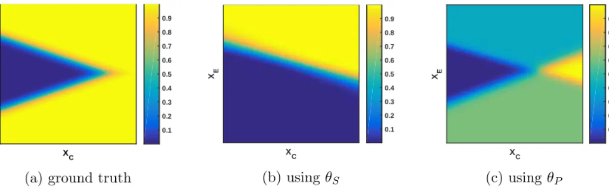
XC XE 0.1 0.2 0.3 0.4 0.5 0.6 0.7 0.8 0.9
(a) ground truth
XC XE 0.1 0.2 0.3 0.4 0.5 0.6 0.7 0.8 0.9 (b) usingθS XC XE 0.1 0.2 0.3 0.4 0.5 0.6 0.7 0.8 0.9 (c) usingθP
Figure 12: Visualization of the probabilistic conditional P(Y = 1|XC, XE) under
model-misspecification, and its Bayesian approximations withnS= 8,nT = 256, corresponding to
the posteriors shown in Fig. 11b. Both XC and XE range from -10 to 10.
Figures 9c and 10c). Moreover, with a Bayesian approach to model misspecification and given 8 labelled observations the peak error reached is about 1.5% lower than with maximum likelihood. FornS = 64 this difference rises to 2.5% in absolute error rate.
Fig. 11 shows two examples of posterior distributions overθS,θW S, andθP given labelled
and unlabelled training data, along with the true parameter values marked by red lines. (Note, however, that the role of µ1 changes between correct and incorrect models, see
Section 4.3 for details.) For a correct model and given 8 labelled and 1024 unlabelled data (Fig. 11a), the posterior over θP, unlike those over θS and θW S, is approximately centred
around the true parameter values. Moreover, it is more spiked as indicated by the scaling of axes. Under model-misspecification as shown in Fig. 11b, on the other hand, the posterior over θP appears to be bimodal with respect toµ0 and µ1, whereas posteriors over θS and
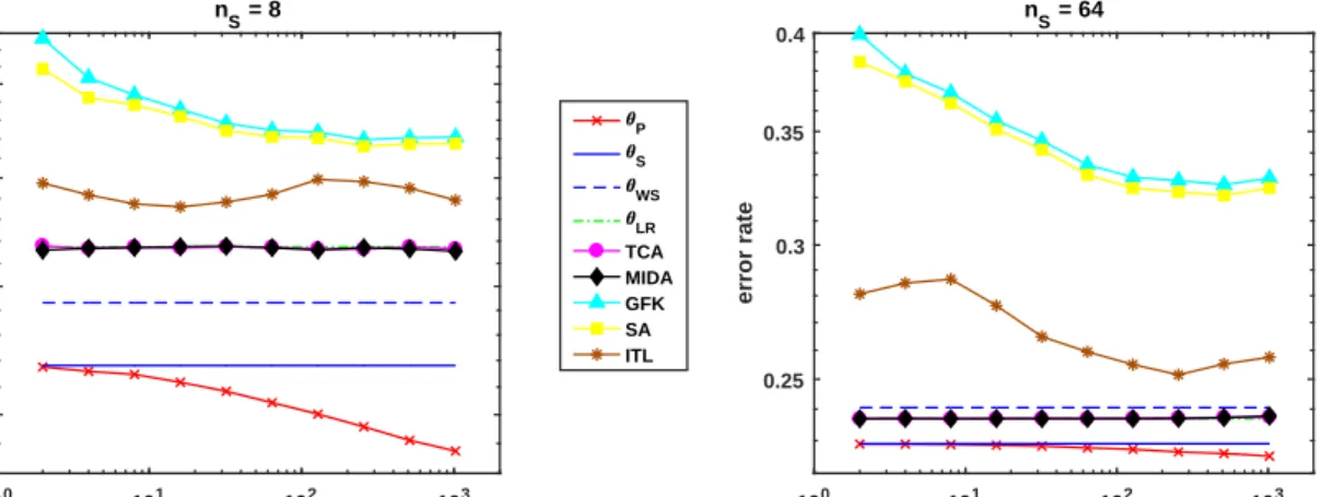
100 101 n 102 103 T 0.25 0.3 0.35 0.4 error rate nS = 8 P S WS LR TCA MIDA GFK SA ITL 100 101 n 102 103 T 0.25 0.3 0.35 0.4 error rate nS = 64
Figure 13: Comparison of our pooled ML estimator with feature-transformation DA meth-ods on synthetic classification data sets with 8 (left) and 64 (right) labelled training exam-ples. Results of TCA and θLR mostly coincide with MIDA and are thus hard to see.
The decision surfaces, P(Y = 1|XC, XE), resulting from the different posteriors in
Fig. 11b are shown in Fig. 12. It also contains the ground truth as used for generating the data in Fig. 5b. As can be seen, the true decision boundary, P(Y = 1|XC, XE) = 0.5, is
formed by two straight lines separating the“Y = 0-cluster” from the Gaussian mixture for
Y = 1. The decision boundary found usingθS corresponds to one of these linear segments,
whereas that found using θP is more differentiated. It appears to be the average of both
linear segments taken individually, resulting in class probabilities close to 0.5 over a wide range of (XC, XE). This observation is consistent with the bimodal posterior overµ0andµ1
found forθP in Fig. 11b, with each mode corresponding to one of the two linear boundaries.
Finally, a comparison of our pooled-data maximum likelihood estimator with logistic regression models trained after different feature transformations is shown in Fig. 13. For 8 labelled examples (left), estimators based on the submodels P(Y|XC) and P(XE|Y) (θS,
θW S, θP) outperform the remaining ones, which train one model on the joint feature set;
for nS = 64, this holds only for θS, and θP. Across both settings, TCA and MIDA lead
to almost identical results as θLR, while ITL, SA, and GFK yield the highest errors. Our
pooled estimator θP is the only one which is strictly improving with more unlabelled data
throughout; however, this improvement is very slim in the case ofnS = 64.
5.2 Synthetic Regression Results
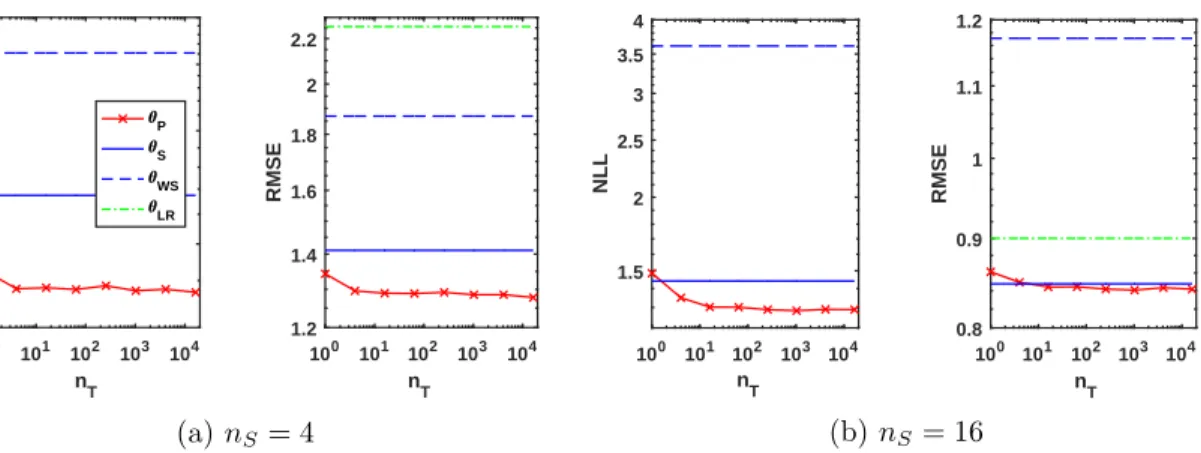
On the synthetic regression data set we perform maximum likelihood estimation and in-vestigate the effect of the interpolating hyperparameter λfurther. Figure 14 shows results for using λ = 0.8 given 4 (a) or 16 (b) labelled training points. As in Fig. 9 (top) with error rate, also for regression with a correct model the surrogate loss curve aligns well with the RMSE. For both values ofnS,θS performs better than θW S. The pooled estimator θP
achieves the lowest RMSE overall and quickly improves uponθS given only a few unlabelled
observations. However, adding more unlabelled data beyondnT >10 does not lead to any
100 101 102 103 104 nT 5 10 15 20 NLL 100 101 102 103 104 nT 1.2 1.4 1.6 1.8 2 2.2 RMSE P S WS LR (a)nS = 4 100 101 102 103 104 n T 1.5 2 2.5 3 3.5 4 NLL 100 101 102 103 104 nT 0.8 0.9 1 1.1 1.2 RMSE (b)nS = 16
Figure 14: Regression results using maximum likelihood estimates with λ= 0.8.
results in a reduction of about 0.1 in RMSE compared to θS. For nS = 16, on the other
hand, this gain is at least an order of magnitude smaller and thus negligible.
The same experiment as is Fig. 14a is repeated in Fig. 15, but this time withλ= nS
nS+nT
(as used for classification). Learning curves of θP (top row) for both NLL and RMSE
decrease initially, quickly reach a minimum at nT = 2, and then rise again leading to
increasingly worsened performance as more unlabelled data is added. For the minimum at nT = 2 and another point at nT = 128 (black arrows), example model fits (lines) are
shown in the middle and bottom rows, respectively. With 2 unlabelled points (middle row), all estimators fit the submodel XE|Y well, but the line fits of θP to XE|XC and Y |XC
are closer to the true model than those of θS and θW S. For nT = 128 (bottom row), all
estimators result in a decent fit toXE|XC withθP almost coinciding with the true model.
The two submodels Y |XC and XE|Y, however, are fitted very poorly by θP, as opposed
toθS and θW S.
5.3 Real-Data Regression Results
On the real-world data sets, we compare the performance of our approach using maximum likelihood estimation with linear regression models trained after different feature transfor-mations. Results from using λ= 0.8 on D1 and D2 are shown in Fig. 16. As can be seen, RMSEs of all methods are much lower on D1 than on D2 supporting our claim that D2 is
the more challenging one.
On D1 with nS = 4 (a), both θS and θP outperform the structure-agnostic feature
transformation methods; θP reaches the lowest RMSE of a little under 0.6—an absolute
improvement of 0.1 over θS with an RMSE of 0.7. For smallnT, MIDA outperforms TCA,
GFK, and SA but for large nT all feature tranformation methods converge in RMSE to
the linear regression modelθLR (coinciding with TCA). With 16 labelled examples (b), on
the other hand, all feature transformation methods except GFK outperform θS and θP,
with MIDA achieving the lowest RMSE, followed by TCA andθLR. SA and GFK lead to
the highest errors on D1, especially for small nT, but both are strictly improving as more
100 101 n 102 103 T 1.4 1.6 1.8 2 2.2 2.4 RMSE 100 101 n 102 103 T 100 101 102 NLL 0 1 2 3 4 X C -10 -5 0 5 10 15 Y 2 4 6 8 Y -20 -15 -10 -5 X E -2 0 2 4 X C -40 -20 0 20 40 X E S WS P true Source Target -2 -1 0 1 2 3 XC -4 -2 0 2 4 6 Y -2 -1 0 1 2 3 Y -10 -5 0 5 X E -4 -2 0 2 4 X C -20 -10 0 10 X E
Figure 15: ML regression results with nS = 4 andλ= n nS
S+nT, showing learning curves of
NLL and RMSE vsnT (top). Arrows marknT = 2 withλ= 32, andnT = 128 withλ≈0.03
100 101 102 103 nT 0.6 0.7 0.8 0.9 1 1.1 1.2 1.3 1.4 RMSE P S LR TCA MIDA GFK SA (a)D1: nS = 4 100 101 102 103 n T 0.3 0.4 0.5 0.6 0.7 0.8 0.9 1 1.1 RMSE (b)D1: nS = 16 100 101 102 103 n T 4 4.2 4.4 4.6 4.8 5 5.2 5.4 5.6 5.8 RMSE (c)D2: nS = 4 100 101 102 103 n T 3.8 4 4.2 4.4 4.6 4.8 5 5.2 5.4 RMSE (d)D2: nS = 16 Figure 16: Regression learning curves for the real data setsD1 andD2with 4 and 16 labelled source observations. Throughout, we usedλ= 0.8 and fitted an (unrestricted) linear model in log-space, see Fig. 7. θLR is not visible as its curve coincides with that of TCA here.
On D2, GFK, despite leading to the worst results on D1, achieves the lowest error for both settings, closely followed by SA. As onD1, both show a monotonic decrease in RMSE with respect to nT, which is not the case for MIDA on either of the data sets. Both θS
and our pooled estimator θP show poor performance on D2, and, as opposed to the other
methods, do not experience improvements in RMSE asnS is increased from 4 to 16.
In the case of D2, we also analyse the effect of additional model restrictions in Fig. 17, considering both λ = 0.8 and λ = nS
nS+nT. Restricting the two linear submodels used in
θS and θP to have negative slope (capturing the inverse relationship between the involved
proteins) leads to considerably lower RMSEs. Unlike their unrestricted counterparts in Fig. 16, the restricted versions of θS and θP clearly outperform the feature tranformation
methods to which no restrictions were applied (to be discussed further later on).
Forλ= 0.8,θP consistently performs better thanθS by an absolute difference in RMSE
of roughly 0.1. However, this difference can be achieved using as little as 2 unlabelled data points beyond which learning curves for θP seem to remain constant; this can also be
observed in Fig. 16, where λ= 0.8 was used throughout.
Forλ= nS
nS+nT, on the other hand, learning curves ofθP show more complex behaviour.
For both 4 (b) and 16 (d) labelled training examples, RMSE initially decreases, then reaches a minimum, and eventually increases again. FornS = 4, though, this minimum occurs much
sooner so that an initial improvement compared to using λ = 0.8 as in (a) is almost not noticeable; for large nT the learning curve in (b) even crosses that of θS attaining a higher
maximum RMSE. WithnS= 16 (d), the minimum occurs much later leading to considerable