Evolving Data Streams
Albert Bifet1, Geoff Holmes1, Bernhard Pfahringer1, and Ricard Gavald`a2 1
University of Waikato, Hamilton, New Zealand
{abifet,geoff,bernhard}@cs.waikato.ac.nz 2
Universitat Polit`ecnica de Catalunya, Barcelona, Spain
{gavalda}@lsi.upc.edu
Abstract. We propose two new improvements for bagging methods on evolving data streams. Recently, two new variants of Bagging were pro-posed:ADWIN Bagging and Adaptive-Size Hoeffding Tree (ASHT) Bag-ging. ASHT Bagging uses trees of different sizes, andADWIN Bagging uses ADWIN as a change detector to decide when to discard underperforming ensemble members. We improveADWIN Bagging using Hoeffding Adap-tive Trees, trees that can adapAdap-tively learn from data streams that change over time. To speed up the time for adapting to change of Adaptive-Size Hoeffding Tree (ASHT) Bagging, we add an error change detector for each classifier. We test our improvements by performing an evaluation study on synthetic and real-world datasets comprising up to ten million examples.
1
Introduction
Data streams pose several challenges on data mining algorithm design. First, algorithms must make use of limited resources (time and memory). Second, by necessity they must deal with data whose nature or distribution changes over time. In turn, dealing with time-changing data requires strategies for detecting and quantifying change, forgetting stale examples, and for model revision. Fairly generic strategies exist for detecting change and deciding when examples are no longer relevant. Model revision strategies, on the other hand, are in most cases method-specific.
The following constraints apply in the Data Stream model:
1. Data arrives as a potentially infinite sequence. Thus, it is impossible to store it all. Therefore, only a small summary can be computed and stored. 2. The speed of arrival of data is fast, so each particular element has to be
processed essentially in real time, and then discarded.
3. The distribution generating the items may change over time. Thus, data from the past may become irrelevant (or even harmful) for the current prediction. Under these constraints the main properties of an ideal classification method are the following: high accuracy and fast adaption to change, low computational
cost in both space and time, theoretical performance guarantees, and a minimal number of parameters.
Ensemble methods are combinations of several models whose individual pre-dictions are combined in some manner (for example, by averaging or voting) to form a final prediction. Often, ensemble learning classifiers provide superior predictive performance and they are easier to scale and parallelize than single classifier methods.
In [6] two new state-of-the-art bagging methods were presented: ASHT Bag-ging using trees of different sizes, andADWIN Bagging using a change detector to decide when to discard underperforming ensemble members. This paper improves on ASHT Bagging by speeding up the time taken to adapt to changes in the distribution generating the stream. It improves onADWIN Bagging by employing Hoeffding Adaptive Trees, trees that can adaptively learn from evolving data streams. The paper is structured as follows: the state-of-the-art Bagging meth-ods are presented in Section 2. Improvements to these methmeth-ods are presented in Section 3. An experimental evaluation is conducted in Section 4. Finally, con-clusions and suggested items for future work are presented in Section 5.
2
Previous Work
2.1 Bagging using trees of different size (ASHT Bagging)
T1 T2 T3 T4
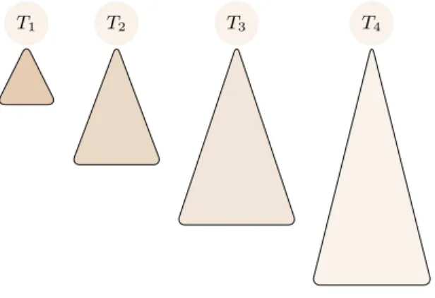
Fig. 1.An ensemble of trees of different size
In [6], a new method of bagging was presented using Hoeffding Trees of different sizes. A Hoeffding tree [10] is an incremental, anytime decision tree induction algorithm that is capable of learning from massive data streams, as-suming that the distribution generating examples does not change over time. Hoeffding trees exploit the fact that a small sample can often be enough to choose an optimal splitting attribute. This idea is supported mathematically by
the Hoeffding bound, which quantifies the number of observations (in our case, examples) needed to estimate some statistics within a prescribed precision (in our case, the goodness of an attribute). More precisely, the Hoeffding bound states that with probability 1−δ, the true mean of a random variable of range
R will not differ from the estimated mean afternindependent observations by more than:
=
r
R2ln(1/δ) 2n .
A theoretically appealing feature of Hoeffding Trees not shared by many other incremental decision tree learners is that it has sound theoretical guarantees of performance. IADEM-2 [9] uses Chernoff and Hoeffding bounds to give simi-lar guarantees. Using the Hoeffding bound one can show that the output of a Hoeffding tree is asymptotically nearly identical to that of a non-incremental learner using infinitely many examples. See [10] for details.
The Adaptive-Size Hoeffding Tree (ASHT) is derived from the Hoeffding Tree algorithm with the following differences:
– it has a value for the maximum number of split nodes, orsize
– after one node splits, if the number of split nodes of the ASHT tree is higher than the maximum value, then it deletes some nodes to reduce its size When the tree size exceeds the maximun size value, there are two different delete options:
– delete the oldest node, the root, and all of its children except the one where the split has been made. After that, the root of the child not deleted becomes the new root.
– delete all the nodes of the tree, that is, reset the tree to the empty tree The intuition behind this method is as follows: smaller trees adapt more quickly to changes, and larger trees perform better during periods with little or no change, simply because they were built on more data. Trees limited to size s will be reset about twice as often as trees with a size limit of 2s. This creates a set of different reset-speeds for an ensemble of such trees, and therefore a subset of trees that are a good approximation for the current rate of change. It is important to note that resets will happen all the time, even for stationary datasets, but this behaviour should not have a negative impact on the ensemble’s predictive performance.
In [6] a new bagging method was presented that uses these Adaptive-Size Hoeffding Trees and that sets the size for each tree. The maximum allowed size for then-th ASHT tree is twice the maximum allowed size for the (n−1)-th tree. Moreover, each tree has a weight proportional to the inverse of the square of its error, and it monitors its error with an exponential weighted moving average (EWMA) withα=.01. The size of the first tree is 2.
With this new method, the authors attempted to improve bagging perfor-mance by increasing tree diversity. It has been observed [18] that boosting tends to produce a more diverse set of classifiers than bagging, and this has been cited as a factor in increased performance.
2.2 Bagging using ADWIN (ADWIN Bagging)
ADWIN [4] is a change detector and estimator that solves in a well-specified way
the problem of tracking the average of a stream of bits or real-valued numbers.
ADWIN keeps a variable-length window of recently seen items, with the
prop-erty that the window has the maximal length statistically consistent with the hypothesis “there has been no change in the average value inside the window”.
More precisely, an older fragment of the window is dropped if and only if there is enough evidence that its average value differs from that of the rest of the window. This has two consequences: first, that change is reliably declared whenever the window shrinks; and second, that at any time the average over the existing window can be reliably taken as an estimate of the current average in the stream (barring a very small or very recent change that is still not statistically visible). A formal and quantitative statement of these two points (in the form of a theorem) appears in [4].
ADWIN is parameter- and assumption-free in the sense that it automatically
detects and adapts to the current rate of change. Its only parameter is a confi-dence boundδ, indicating how confident we want to be in the algorithm’s output, a property inherent to all algorithms dealing with random processes.
Also important for our purposes,ADWIN does not maintain the window ex-plicitly, but compresses it using a variant of the exponential histogram technique. This means that it keeps a window of length W using onlyO(logW) memory andO(logW) processing time per item.
Bagging usingADWIN is implemented asADWIN Bagging where the Bagging method is the online bagging method of Oza and Rusell [20] with the addition of
theADWIN algorithm as a change detector. The base classifiers used are Hoeffding
Trees. When a change is detected, the worst classifier of the ensemble of classifiers is removed and a new classifier is added to the ensemble.
3
Improvements for Adaptive Bagging Methods
In this section we propose two new improvements for the adaptive bagging meth-ods explained in the previous section.
3.1 ADWIN bagging using Hoeffding Adaptive Trees
The basic idea is to use Hoeffding trees, that are able to adapt to distribution changes instead of non-adaptive Hoeffding trees as the base classifier for the bagging ensemble method. We use the Hoeffding Adaptive Trees proposed in [5], where a new method for managing alternate trees is proposed. The general idea is simple: we placeADWIN instances at every node that will raise an alert whenever something worth attention happens at the node.
We use the variant of theHoeffding Adaptive Treealgorithm (HAT for short) that uses ADWIN as a change detector. It uses one instance of ADWIN in each node, as a change detector, to monitor the classification error rate at that node.
A significant increase in that rate indicates that the data is changing with respect to the time at which the subtree was created. This was the approach used by Gamaet al.in [12], using another change detector.
When any instance of ADWIN at a node detects change, we create a new alternate tree without splitting any attribute. Using two ADWIN instances at every node, we monitor the average error of the subtree rooted at this node and the average error of the new alternate subtree. When there is enough evidence (as witnessed by ADWIN) that the new alternate tree is doing better than the original decision subtree, we replace the original decision subtree by the new alternate subtree.
3.2 DDM bagging using trees of different size
We improve bagging using trees of different size, by adding a change detector for each tree in the ensemble to speed up the adaption to the evolving stream.
A change detector or drift detection method is an algorithm that takes as input a sequence of numbers and emits a signal when the distribution of its input changes. There are many such methods such as the CUSUM Test, the Geometric Moving Average test, etc. Change detection is not an easy task, since a fundamental limitation exists: the design of a change detector is a compromise between detecting true changes and avoiding false alarms. See [14] and [3] for a more detailed survey of change detection methods.
We use two drift detection methods (DDM and EDDM) proposed by Gama et al. [11] and Baena-Garc´ıa et al. [2]. These methods control the number of errors produced by the learning model during prediction. They compare the statistics of two windows: the first contains all of the data, and the second contains only the data from the beginning until the number of errors increases. Their methods do not store these windows in memory. They keep only statistics and a window of recent errors data.
The drift detection method (DDM) uses the number of errors in a sample ofn
examples, modelled by a binomial distribution. For each pointiin the sequence that is being sampled, the error rate is the probability of misclassifying (pi), with standard deviation given by si =
p
pi(1−pi)/i. They assume (as stated in the PAC learning model [19]) that the error rate of the learning algorithm (pi) will decrease while the number of examples increases if the distribution of the examples is stationary. A significant increase in the error of the algorithm, suggests that the class distribution is changing and, hence, the actual decision model is supposed to be inappropriate. Thus, they store the values ofpi andsi whenpi+sireaches its minimum value during the process (obtainingppmin and
smin). It then checks when the following conditions are triggered:
– pi+si≥pmin+2·sminfor the warning level. Beyond this level, the examples are stored in anticipation of a possible change of context.
– pi+si ≥ pmin+ 3·smin for the drift level. Beyond this level the concept drift is supposed to be true, the model induced by the learning method is reset and a new model is learnt using the examples stored since the warning level triggered. The values forpminand sminare reset too.
This approach is good at detecting abrupt changes and gradual changes when the gradual change is not very slow, but has difficulties when the change is gradual and slow. In that case, the examples will be stored for a long time, the drift level then takes too long to trigger and the examples in memory can be exceeded.
Baena-Garc´ıa et al. proposed a new method EDDM [2] in order to improve DDM. It is based on the estimated distribution of the distances between classi-fication errors. The window resize procedure is governed by the same heuristics.
4
Comparative Experimental Evaluation
MassiveOnlineAnalysis (MOA) [16] is a software environment for implement-ing algorithms and runnimplement-ing experiments for online learnimplement-ing from data streams. The data stream evaluation framework and all algorithms evaluated in this paper were implemented in the Java programming language extending the MOA soft-ware. MOA includes a collection of offline and online methods as well as tools for evaluation. In particular, it implements boosting, bagging, and Hoeffding Trees, all with and without Na¨ıve Bayes classifiers at the leaves.
One of the key data structures used in MOA is the description of an example from a data stream. This structure borrows from WEKA, where an example is represented by an array of double precision floating point values. This provides freedom to store all necessary types of value – numeric attribute values can be stored directly, and discrete attribute values and class labels are represented by integer index values that are stored as floating point values in the array. Double precision floating point values require storage space of 64 bits, or 8 bytes. This detail can have implications for memory usage.
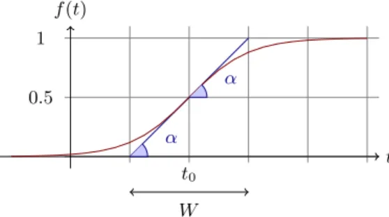
We use the new experimental framework for concept drift presented in [6]. Considering data streams as data generated from pure distributions, we can model a concept drift event as a weighted combination of two pure distributions that characterizes the target concepts before and after the drift. This framework defines the probability that every new instance of the stream belongs to the new concept after the drift. It uses the sigmoid function, as an elegant and practical solution.
We see from Figure 2 that the sigmoid function
f(t) = 1/(1 + e−s(t−t0))
has a derivative at the point t0 equal tof0(t0) = s/4. The tangent of angle α is equal to this derivative, tanα=s/4. We observe that tanα= 1/W, and as
s= 4 tanαthens= 4/W. So the parametersin the sigmoid gives the length of
W and the angleα. In this sigmoid model we only need to specify two parameters :t0the point of change, and W the length of change.
Definition 1. Given two data streams a, b, we define c=a⊕W
t0 b as the data stream built joining the two data streamsaandb, wheret0is the point of change,
t f(t) α α t0 W 0.5 1
Fig. 2.A sigmoid functionf(t) = 1/(1 + e−s(t−t0)).
– Pr[c(t) =a(t)] = e−4(t−t0)/W/(1 + e−4(t−t0)/W)
– Pr[c(t) =b(t)] = 1/(1 + e−4(t−t0)/W).
In order to create a data stream with multiple concept changes, we can build new data streams joining different concept drifts:
(((a⊕W0 t0 b)⊕ W1 t1 c)⊕ W2 t2 d). . .
4.1 Datasets for concept drift
Synthetic data has several advantages – it is easier to reproduce and there is little cost in terms of storage and transmission. For this paper we use the data generators most commonly found in the literature.
SEA Concepts Generator This artificial dataset contains abrupt concept drift, first introduced in [23]. It is generated using three attributes, where only the two first attributes are relevant. All the attributes have values between 0 and 10. The points of the dataset are divided into 4 blocks with different concepts. In each block, the classification is done usingf1+f2≤θ, wheref1 andf2represent the first two attributes andθis a threshold value. The most frequent values are 9, 8, 7 and 9.5 for the data blocks. In our framework, SEA concepts are defined as follows:
(((SEA9⊕Wt0 SEA8)⊕ W
2t0SEA7)⊕ W
3t0SEA9.5)
Rotating Hyperplane It was used as testbed for CVFDT versus VFDT in [17]. A hyperplane ind-dimensional space is the set of pointsxthat satisfy
d X i=1 wixi =w0= d X i=1 wi
wherexi, is the ith coordinate ofx. Examples for whichP d
i=1wixi≥w0are labeled positive, and examples for whichPd
i=1wixi < w0 are labeled nega-tive. Hyperplanes are useful for simulating time-changing concepts, because
we can change the orientation and position of the hyperplane in a smooth manner by changing the relative size of the weights. We introduce change to this dataset adding drift to each weight attributewi=wi+dσ, whereσis the probability that the direction of change is reversed anddis the change applied to every example.
Random RBF Generator This generator was devised to offer an alternate complex concept type that is not straightforward to approximate with a decision tree model. The RBF (Radial Basis Function) generator works as follows: A fixed number of random centroids are generated. Each center has a random position, a single standard deviation, class label and weight. New examples are generated by selecting a center at random, taking weights into consideration so that centers with higher weight are more likely to be chosen. A random direction is chosen to offset the attribute values from the central point. The length of the displacement is randomly drawn from a Gaussian distribution with standard deviation determined by the chosen centroid. The chosen centroid also determines the class label of the example. This effec-tively creates a normally distributed hypersphere of examples surrounding each central point with varying densities. Only numeric attributes are gener-ated. Drift is introduced by moving the centroids with constant speed. This speed is initialized by a drift parameter.
LED Generator This data source originates from the CART book [7]. An implementation in C was donated to the UCI [1] machine learning repository by David Aha. The goal is to predict the digit displayed on a seven-segment LED display, where each attribute has a 10% chance of being inverted. It has an optimal Bayes classification rate of 74%. The particular configuration of the generator used for experiments (led) produces 24 binary attributes, 17 of which are irrelevant.
Data streams may be considered infinite sequences of (x, y) wherexis the feature vector andythe class label. Zhang et al. [24] observe thatp(x, y) =p(x|t)·p(y|x) and categorize concept drift in two types:
– Loose Concept Drifting (LCD) when concept drift is caused only by the change of the class prior probabilityp(y|x),
– Rigorous Concept Drifting (RCD)when concept drift is caused by the change of the class prior probabilityp(y|x) and the conditional probabilityp(x|t) Note that the Random RBF Generator has RCD drift, and the rest of the dataset generators have LCD drift.
4.2 Real-World Data
It is not easy to find large real-world datasets for public benchmarking, espe-cially with substantial concept change. The UCI machine learning repository [1] contains some real-world benchmark data for evaluating machine learning tech-niques. We consider three of the largest: Forest Covertype, Poker-Hand, and Electricity.
Hyperplane Hyperplane Drift .0001 Drift .001
Time Acc. Mem. Time Acc. Mem. BagADWIN 10 HAT 3025.87 91.36±0.13 9.91 2834.85 91.12±0.15 1.23 DDM Bag10 ASHT W 1321.64 91.60±0.09 0.85 1351.1691.43±0.07 2.10 EDDM Bag10 ASHT W 1362.31 91.43±0.13 3.15 1371.46 91.17±0.11 2.77 NaiveBayes 86.97 83.40±2.11 0.01 86.87 77.54±2.93 0.01 NBADWIN 308.85 91.30±0.90 0.06 295.19 90.58±0.59 0.06 HT 157.71 86.09±1.60 9.57 159.43 82.99±1.88 10.41 HT DDM 174.10 89.36±0.24 0.04 180.51 89.07±0.26 0.01 HT EDDM 207.47 88.73±0.38 13.23 193.07 87.97±0.51 2.52 HAT 500.81 89.75±0.25 1.72 431.6 89.40±0.30 0.15 BagADWIN 10 HT 1306.22 91.18±0.12 11.40 1308.08 90.86±0.15 5.52 Bag10 HT 1236.92 87.07±1.64 108.75 1253.07 84.13±1.79 114.14 Bag10 ASHT 1060.37 90.85±0.53 2.68 1070.44 90.39±0.33 2.69 Bag10 ASHT W 1055.87 91.38±0.26 2.68 1073.96 91.01±0.18 2.69 Bag10 ASHT R 995.06 91.44±0.09 2.95 1016.48 91.17±0.12 2.14 Bag10 ASHT W+R 996.5291.62±0.08 2.95 1024.02 91.40±0.10 2.14 Bag5 ASHT W+R 551.53 90.83±0.06 0.08 562.09 90.75±0.06 0.09 OzaBoost 974.69 86.68±1.19 130.00 959.14 84.47±1.49 123.75 Table 1.Comparison of algorithms. Accuracy is measured as the final percentage of examples correctly classified over the 1 or 10 million test/train interleaved evaluation. Time is measured in seconds, and memory in MB. The best individual accuracies are indicated in boldface.
Forest Covertype Contains the forest cover type for 30 x 30 meter cells ob-tained from US Forest Service (USFS) Region 2 Resource Information Sys-tem (RIS) data. It contains 581,012 instances and 54 attributes, and it has been used in several papers on data stream classification [13, 21].
Poker-Hand Consists of 1,000,000 instances and 11 attributes. Each record of the Poker-Hand dataset is an example of a hand consisting of five playing cards drawn from a standard deck of 52. Each card is described using two attributes (suit and rank), for a total of 10 predictive attributes. There is one Class attribute that describes the “Poker Hand”. The order of cards is important, which is why there are 480 possible Royal Flush hands instead of 4.
Electricity Is another widely used dataset described by M. Harries [15] and analysed by Gama [11]. This data was collected from the Australian New South Wales Electricity Market. In this market, the prices are not fixed and are affected by demand and supply of the market. The prices in this market are set every five minutes. The ELEC dataset contains 45,312 instances. Each example of the dataset refers to a period of 30 minutes, i.e. there are 48 instances for each time period of one day. The class label identifies the change of the price related to a moving average of the last 24 hours. The class
SEA RandomRBF
W= 50000 No Drift
50 centers
Time Acc. Mem. Time Acc. Mem. BagADWIN 10 HAT 154.9188.88±0.05 2.35 5378.75 95.34±0.06 119.17 DDM Bag10 ASHT W 44.02 88.72±0.05 0.65 1230.43 93.09±0.05 3.21 EDDM Bag10 ASHT W 48.95 88.60±0.05 0.90 1317.58 93.28±0.03 3.76 NaiveBayes 5.52 84.60±0.03 0.00 111.12 72.04±0.02 0.01 NBADWIN 12.40 87.83±0.07 0.02 396.01 72.04±0.02 0.08 HT 7.20 85.02±0.11 0.33 154.67 93.80±0.10 6.86 HT DDM 7.88 88.17±0.18 0.16 185.15 93.77±0.12 13.72 HT EDDM 8.52 87.87±0.22 0.06 185.89 93.75±0.14 13.81 HAT 20.96 88.40±0.07 0.18 794.48 93.80±0.10 9.28 BagADWIN 10 HT 53.15 88.58±0.10 0.88 1238.50 95.34±0.06 67.79 Bag10 HT 30.88 85.38±0.06 3.36 995.4695.35±0.05 71.26 Bag10 ASHT 35.30 88.02±0.08 0.91 1009.62 80.08±0.14 3.73 Bag10 ASHT W 35.69 88.27±0.08 0.91 986.90 92.84±0.05 3.73 Bag10 ASHT R 33.74 88.38±0.06 0.84 913.74 90.03±0.03 2.65 Bag10 ASHT W+R 33.56 88.51±0.06 0.84 925.65 92.85±0.05 2.65 Bag5 ASHT W+R 20.00 87.80±0.06 0.05 536.61 80.82±0.07 0.06 OzaBoost 39.97 86.64±0.06 4.00 964.75 94.85±0.03 206.60 Table 2.Comparison of algorithms. Accuracy is measured as the final percentage of examples correctly classified over the 1 or 10 million test/train interleaved evaluation. Time is measured in seconds, and memory in MB.
level only reflect deviations of the price on a one day average and removes the impact of longer term price trends.
The size of these datasets is small, compared to tens of millions of training examples of synthetic datasets: 45,312 for ELEC dataset, 581,012 for Cover-Type, and 1,000,000 for Poker-Hand. Another important fact is that we do not know when drift occurs or indeed if there is any drift. We may simulate RCD concept drift, joining the three datasets, merging attributes, and supposing that each dataset corresponds to a different concept.
CovPokElec = (CoverType⊕5581,000,012Poker)⊕51,,000000,000ELEC
As all examples need to have the same number of attributes, we simple con-catenate all the attributes, and set the number of classes to the maximum num-ber of classes of all the datasets. The attribute values for a type not currently selected is a constant one, for example, zero.
4.3 Results
We use the datasets for evaluation explained in the previous sections. The exper-iments were performed on a 2.0 GHz Intel Core Duo PC machine with 2 Gigabyte
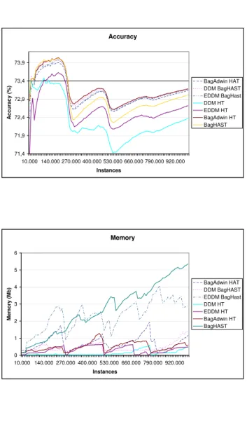
Accuracy 71,4 71,9 72,4 72,9 73,4 73,9 10.000 140.000 270.000 400.000 530.000 660.000 790.000 920.000 Instances A c c u ra c y ( %
) BagAdwin HATDDM BagHAST
EDDM BagHast DDM HT EDDM HT BagAdwin HT BagHAST Memory 0 1 2 3 4 5 6 10.000 140.000 270.000 400.000 530.000 660.000 790.000 920.000 Instances M e m o ry ( M b
) BagAdwin HATDDM BagHAST
EDDM BagHast DDM HT EDDM HT BagAdwin HT BagHAST RunTime 0 50 100 150 200 250 300 350 400 10.000 140.000 270.000 400.000 530.000 660.000 790.000 920.000 Instances T im e ( s e c .) BagAdwin HAT DDM BagHAST EDDM BagHast DDM HT EDDM HT BagAdwin HT BagHAST
RandomRBF RandomRBF Drift .0001 Drift .001
50 centers 50 centers
Time Acc. Mem. Time Acc. Mem. BagADWIN 10 HAT 2706.9185.98±0.04 0.51 1976.62 67.20±0.03 0.10 DDM Bag10 ASHT W 1349.65 83.77±0.15 0.53 1441.2270.01±0.31 3.09 EDDM Bag10 ASHT W 1366.65 84.20±0.46 0.71 1422.31 69.99±0.35 0.71 NaiveBayes 111.47 53.21±0.02 0.01 113.37 53.18±0.02 0.01 NBADWIN 272.58 68.05±0.02 0.05 249.1 62.19±0.02 0.04 HT 189.25 63.40±0.10 9.86 186.47 55.40±0.02 8.90 HT DDM 199.95 76.40±0.08 0.02 206.41 62.40±1.91 0.03 HT EDDM 214.55 76.39±0.57 0.09 203.41 63.23±0.71 0.02 HAT 413.53 79.12±0.08 0.09 294.94 65.32±0.03 0.01 BagADWIN 10 HT 1326.12 85.28±0.03 0.26 1354.03 67.20±0.03 0.03 Bag10 HT 1362.66 71.01±0.06 106.20 1240.89 58.17±0.03 88.52 Bag10 ASHT 1124.40 74.76±0.04 3.05 1133.51 66.25±0.02 3.10 Bag10 ASHT W 1104.03 75.55±0.05 3.05 1106.26 66.81±0.02 3.10 Bag10 ASHT R 1069.76 83.48±0.03 3.74 1085.99 67.78±0.02 2.35 Bag10 ASHT W+R 1068.59 84.20±0.03 3.74 1101.10 69.14±0.02 2.35 Bag5 ASHT W+R 557.20 79.45±0.06 0.09 587.46 67.53±0.02 0.10 OzaBoost 1312.00 71.64±0.07 105.94 1266.75 58.21±0.05 88.36 Table 3.Comparison of algorithms. Accuracy is measured as the final percentage of examples correctly classified over the 1 or 10 million test/train interleaved evaluation. Time is measured in seconds, and memory in MB.
main memory, running Ubuntu 8.10. The evaluation methodology used was In-terleaved Test-Then-Train on 10 runs: every example was used for testing the model before using it to train. This interleaved test followed by train procedure was carried out on 10 million examples from the hyperplane and RandomRBF datasets, and one million examples from the SEA dataset. Tables 1, 2 and 3 reports the final accuracy, and speed of the classification models induced on syn-thetic data. Table 4 shows the results for real datasets: Forest CoverType, Poker Hand, and CovPokElec. The results for the Electricity dataset were structurally similar to those for the Forest CoverType dataset and therefore not reported. Additionally, the learning curves and model growth curves for LED dataset are plotted (Figure 3).
The first, and baseline, algorithm (HT) is a single Hoeffding tree, enhanced with adaptive Naive Bayes leaf predictions. Parameter settings arenmin= 1000,
δ = 10−8 and τ = 0.05, as used in [10]. The HT DDM and HT EDDM are Hoeffding Trees with drift detection methods as explained in Section 3.2.
Bag10 is Oza and Russell online bagging using ten classifiers and Bag5 only five. BagADWIN is the online bagging version using ADWIN explained in Sec-tion 2.2. As described earlier, we implemented the following new variants of bagging:
Cover Type Poker CovPokElec Time Acc. Mem. Time Acc. Mem. Time Acc. Mem. BagADWIN 10 HAT 317.75 85.48 0.2 267.4188.63 13.74 1403.4087.16 0.62 DDM Bag10 ASHT W 249.9288.39 6.09 128.17 75.85 1.51 876.18 84.54 19.74 EDDM Bag10 ASHT W 207.10 86.72 0.37 141.96 85.93 12.84 828.63 84.98 48.54 NaiveBayes 31.66 60.52 0.05 13.58 50.01 0.02 91.50 23.52 0.08 NBADWIN 127.34 72.53 5.61 64.52 50.12 1.97 667.52 53.32 14.51 HT 31.52 77.77 1.31 18.98 72.14 1.15 95.22 74.00 7.42 HT DDM 40.26 84.35 0.33 21.58 61.65 0.21 114.72 71.26 0.42 HT EDDM 34.49 86.02 0.02 22.86 72.20 2.30 114.57 76.66 11.15 HAT 55.00 81.43 0.01 31.68 72.14 1.24 188.65 75.75 0.01 BagADWIN 10 HT 247.50 84.71 0.23 165.01 84.84 8.79 911.57 85.95 0.41 Bag10 HT 138.41 83.62 16.80 121.03 87.36 12.29 624.27 81.62 82.75 Bag10 ASHT 213.75 83.34 5.23 124.76 86.80 7.19 638.37 78.87 29.30 Bag10 ASHT W 212.17 85.37 5.23 123.72 87.13 7.19 636.42 80.51 29.30 Bag10 ASHT R 229.06 84.20 4.09 122.92 86.21 6.47 776.61 80.01 29.94 Bag10 ASHT W+R 198.04 86.43 4.09 123.25 86.76 6.47 757.00 81.05 29.94 Bag5 ASHT W+R 116.83 83.79 0.23 57.09 75.87 0.44 363.09 77.65 0.95 OzaBoost 170.73 85.05 21.22 151.03 87.85 14.50 779.99 84.69 105.63 Table 4.Comparison of algorithms on real data sets. Time is measured in seconds, and memory in MB. The results are based on a single run. Unlike synthetic datasets, it is not straightforward to add randomization to real datasets such that meaningful datasets and analysis of performance variances are obtained.
– Bagging ASHT using the DDM drift detection method
– Bagging ASHT using the EDDM drift detection method
In general terms, we observe that ensemble methods perform better than single classifier methods, and that explicit drift detection is better. However, these improvements come at a cost of runtime and memory. In fact, the results indicate that memory is not as big an issue as the runtime accuracy tradeoff. We observe that the variance in accuracy goes up when the drift increases, and vice versa. All classifiers have a small accuracy variance for the dataset RandomRBF with no drift, as shown in Table 2.
RCD drift produces much greater differences than LCD - for example, the best result in Table 3 goes down 16% when increasing the drift from 0.0001 to 0.001 - in Hyperplane the same change in drift elicits only a fractional change in accuracy. For RCD drift all methods drop significantly. The bagging methods have the most to lose and go down between 14-17% (top three) and 10-18% (bottom of table). The base methods have less to lose going down (0-14%).
For all datasets one of the new methods always wins in terms of accuracy. Specifically, on the nine analysed datasets: BagADWIN 10 HAT wins four times out of nine,DDM Bag10 ASHT Wwins three times,DDM Bag10 ASHT Wwins once; this relationship is consistent in the following way: whenever the single HAT
versa. Note that the bad result forDDM Bag10 ASHT Won the Poker dataset must be due to too many false positive drift predictions that wrongly keep the model too small (this can be verified by observing the memory usage in this case), which is mirrored by the behavior of HT DDMon the Poker dataset.
The new improved ensemble methods presented in this paper are slower than the old ones, withBagADWIN 10 HATbeing worst, because it pays twice: through the addition of ADWIN and HAT, the latter being slower than HT by a factor between two and five. Change detection can be time-consuming, the extreme case beingNaive Bayesvs.NBAdwin, whereNaive Bayescan be up to six times faster. However, change detection helps accuracy, with improvements of up to 20 percentage points (see, for example, CovPokElec).
Non-drift-aware non-adaptive ensembles likeBag10 HTandOzaBoostusually need the most memory, sometimes by a very large margin. Bag10 ASHT W+R
needs a lot more memory thanBag5 ASHT W+R, because the last trees in aBag
N ASHT W+R needs as much space as the fullBag N-1 ASHT W+Rensemble.
Recall that data stream evaluation is fundamentally three-dimensional. When adding adaptability to evolving data streams using change detector methods, we increase the run-time, obtaining more accurate methods. For example, adding a change detector DDM to HT, or toBag10 ASHT W, in Table 1, we observe a higher cost in runtime, but also an improvement in accuracy.
5
Conclusions and Future Work
We have presented two new improvements for bagging methods, using Hoeffding Adaptive Trees and change detection methods. In general terms, we observe that using explicit drift detection methods we improve accuracy. However, these improvements come at a cost of runtime and memory. It seems that the cost of improving accuracy in bagging methods for data streams, is large in runtime, but small in memory.
As future work, we would like to build new ensemble methods that perform with an accuracy similar to the methods presented in this paper, but using less runtime. These new methods could be a boosting ensemble method, or a bagging method using new change detection strategies. We think that a boosting method could improve bagging performance by increasing tree diversity, as it is shown by the increased performance of boosting for the traditional batch learning setting. This could be a challenging topic since in [6], the authors didn’t find any boosting method in the literature [20, 22, 8] that outperformed bagging in the streaming setting.
References
[1] A. Asuncion and D. Newman. UCI machine learning repository, 2007.
[2] M. Baena-Garc´ıa, J. del Campo- ´Avila, R. Fidalgo, A. Bifet, R. Gavald`a, and R. Morales-Bueno. Early drift detection method. InFourth International Work-shop on Knowledge Discovery from Data Streams, 2006.
[3] M. Basseville and I. V. Nikiforov. Detection of abrupt changes: theory and appli-cation. Prentice-Hall, Inc., Upper Saddle River, NJ, USA, 1993.
[4] A. Bifet and R. Gavald`a. Learning from time-changing data with adaptive win-dowing. InSIAM International Conference on Data Mining, pages 443–448, 2007. [5] A. Bifet and R. Gavald`a. Adaptive learning from evolving data streams. InIDA,
2009.
[6] A. Bifet, G. Holmes, B. Pfahringer, R. Kirkby, and R. Gavald`a. New ensemble methods for evolving data streams. InKDD ’09. ACM, 2009.
[7] L. Breiman et al. Classification and Regression Trees. Chapman & Hall, New York, 1984.
[8] F. Chu and C. Zaniolo. Fast and light boosting for adaptive mining of data streams. InPAKDD, pages 282–292. Springer Verlag, 2004.
[9] J. del Campo- ´Avila, G. Ramos-Jim´enez, J. Gama, and R. M. Bueno. Improving the performance of an incremental algorithm driven by error margins.Intell. Data Anal., 12(3):305–318, 2008.
[10] P. Domingos and G. Hulten. Mining high-speed data streams. In Knowledge Discovery and Data Mining, pages 71–80, 2000.
[11] J. Gama, P. Medas, G. Castillo, and P. Rodrigues. Learning with drift detection. InSBIA Brazilian Symposium on Artificial Intelligence, pages 286–295, 2004. [12] J. Gama, P. Medas, and R. Rocha. Forest trees for on-line data. In SAC ’04:
Proceedings of the 2004 ACM symposium on Applied computing, pages 632–636, New York, NY, USA, 2004. ACM Press.
[13] J. Gama, R. Rocha, and P. Medas. Accurate decision trees for mining high-speed data streams. InKDD ’03, pages 523–528, August 2003.
[14] F. Gustafsson. Adaptive Filtering and Change Detection. Wiley, 2000.
[15] M. Harries. Splice-2 comparative evaluation: Electricity pricing. Technical report, The University of South Wales, 1999.
[16] G. Holmes, R. Kirkby, and B. Pfahringer. MOA: Massive Online Analysis. http://sourceforge.net/projects/ moa-datastream. 2007.
[17] G. Hulten, L. Spencer, and P. Domingos. Mining time-changing data streams. In KDD’01, pages 97–106, San Francisco, CA, 2001. ACM Press.
[18] D. D. Margineantu and T. G. Dietterich. Pruning adaptive boosting. InICML ’97, pages 211–218, 1997.
[19] T. Mitchell. Machine Learning. McGraw-Hill Education (ISE Editions), October 1997.
[20] N. Oza and S. Russell. Online bagging and boosting. In Artificial Intelligence and Statistics 2001, pages 105–112. Morgan Kaufmann, 2001.
[21] N. C. Oza and S. Russell. Experimental comparisons of online and batch versions of bagging and boosting. InKDD ’01, pages 359–364, August 2001.
[22] R. Pelossof, M. Jones, I. Vovsha, and C. Rudin. Online coordinate boosting. http://arxiv.org/abs/0810.4553, 2008.
[23] W. N. Street and Y. Kim. A streaming ensemble algorithm (SEA) for large-scale classification. In KDD ’01, pages 377–382, New York, NY, USA, 2001. ACM Press.
[24] P. Zhang, X. Zhu, and Y. Shi. Categorizing and mining concept drifting data streams. InKDD ’08, pages 812–820. ACM, 2008.