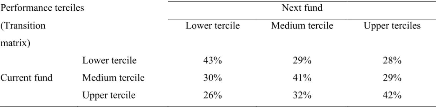
The Performance of Private Equity Funds
Ludovic Phalippou and Oliver Gottschalg
September 2006
Using a unique and comprehensive dataset, we show that the sample of mature private equity funds used in previous research and as an industry benchmark is biased towards better performing funds. We also show that accounting values reported by these mature funds for non-exited investments are substantial and we provide evidence that they mostly represent living dead investments. After correcting for sample bias and overstated accounting values, average fund performance changes from slight overperformance to substantial underperformance of -3.83% per year with respect to the S&P 500. Assuming a typical fee structure, we find that gross-of-fees these funds outperform by 2.96% per year. We conclude that the stunning growth in the amount allocated to this asset class cannot be attributed to genuinely high past performance. We discuss several potentially misleading aspects of standard performance reporting and discuss some of the added benefits of investing in private equity funds as a first step towards an explanation for our results.
JEL: G23, G24
Keywords: Private equity funds, performance Please address all correspondence to: Ludovic Phalippou,
University of Amsterdam, Faculty of Economics and Econometrics, Finance group, 11 Roerterstraat, 1018 Amsterdam, The Netherlands.
Tel: +31 20 525 4153, Email: [email protected]
Oliver Gottschalg is affiliated to the strategy and business policy department at HEC Paris. Financial support from the R&D Department at INSEAD, the Fondation HEC and the Wharton-INSEAD Alliance are gratefully acknowledged. The authors would like to thank Gemma Postlethwaite and Jesse Reyes from Thomson Venture Economics for making this project possible through generous access to their databases. We also thank Bernard Dumas, Alexander Groh, Tim Jenkinson (WFA discussant), Ron Kaniel, Robert Kosowski, Josh Lerner, Dima Leshchinskii, Vinay Nair, Eric Nowak, Andrew Metrick, Manju Puri, Anna Scherbina, Antoinette Schoar, Clemens Sialm (EFA discussant), Per Stromberg, Charles Trzcinka (FFC discussant), Annette Vissing-Jorgensen, Maurizio Zollo and seminar participants at INSEAD, Toulouse Business School, University College Dublin, SIFR-Stockholm, the EFMA meeting in Basle, the CEPR meeting in Gerzensee, the EFA meeting in Moscow, the Frontiers of Finance Conference in Bonaire, the Gutmann Center symposium in Vienna, and the WFA meeting in Keystone for their constructive comments.
The Performance of Private Equity Funds
Using a unique and comprehensive dataset, we show that the sample of mature private equity funds used in previous research and as an industry benchmark is biased towards better performing funds. We also show that accounting values reported by these mature funds for non-exited investments are substantial and we provide evidence that they mostly represent living dead investments. After correcting for sample bias and overstated accounting values, average fund performance changes from slight overperformance to substantial underperformance of -3.83% per year with respect to the S&P 500. Assuming a typical fee structure, we find that gross-of-fees these funds outperform by 2.96% per year. We conclude that the stunning growth in the amount allocated to this asset class cannot be attributed to genuinely high past performance. We discuss several potentially misleading aspects of standard performance reporting and discuss some of the added benefits of investing in private equity funds as a first step towards an explanation for our results.
When The Economist dubbed private equity funds as “Capitalism’s new kings”,1 it was in part commenting on the astonishing growth in the amount of money managed by these funds.2 Indeed, the capital committed to US private equity funds increased from $5 billion in 1980 to $300 billion in 2004, and in the course of the past 25 years, over $1 trillion has passed through the hands of private equity funds (Lerner et al., 2004). Moreover, as many investments are highly levered, the economic impact is even greater than the amounts invested suggest. According to the press, the spectacular growth of this asset class is primarily due to a widely held belief among investors that it has exhibited high performance in the past (see Appendix B). However, and despite the fact that private equity funds represent a major class of financial assets, we are still missing a comprehensive account of the historic performance of private equity funds.
Two partial yet important exceptions are the studies by Ljungqvist and Richardson (2003) and Kaplan and Schoar (2005), which both report that private equity funds outperform the S&P 500. Importantly, the focus of these two studies is not on measuring performance but rather on certain important aspects of investing in private equity funds (e.g. the flow-performance relationship, performance persistence, or determinants of the speed at which capital is invested). One likely explanation for these studies not focusing on performance is data limitations. Indeed, our data show that at least 1,579 funds have been raised between 1980 and 1993. In comparison, Ljungqvist and Richardson (2003) have a sample of 73 funds while Kaplan and Schoar (KS, 2005) have a sample of 639 funds for the same time period.
This paper draws on a unique and comprehensive dataset to investigate whether the historic performance of private equity funds surpasses that of public equity. The data used in this study include an updated version of KS’s dataset, comprised of 852 mature funds for which the cash-flows (to/from investors) are available. Industry-standard performance benchmarks, such as performance statistics published by Thomson Venture Economics as well as the KS performance estimates are based on these “in-sample” funds. The unique feature of our data is that we have, in addition, access to an ‘investment dataset’ with information on the characteristics of most in-sample funds and 727 additional mature “out-of-in-sample” funds. This ‘investment dataset’ includes data on the proportion of the investments exited via either an IPO or an M&A (exit success), which is a widely used proxy for fund performance (e.g. Hochberg, Ljungqvist and Lu,
1 27 November 2004, The Economist.
2 Note that real estate and entrepreneurial investments in non-public companies are sometimes referred to as private
2005). This additional dataset, therefore, enables us to test whether out-of-sample funds are similar to in-sample funds in terms of performance.
We regress exit success on fund characteristics and on a dummy variable that takes the value 1 if the fund is in-sample, and 0 otherwise. This dummy variable is both highly statistically significant (t-stats above 3) and economically significant. A fund that is in-sample is expected to have an additional 6% of invested capital that is exited successfully. Consequently, this result provides a first indication that out-of-sample funds have lower performance than in-sample funds, which suggests that performance estimates based on in-sample funds are overstated.
To assess the magnitude of the corresponding bias in performance estimates, we need to estimate the relationship between exit success and cash-flow based measures of fund performance. Our data offer us this unique opportunity for 618 of the 852 in-sample funds for which both investment data and cash-flow data are available. We find evidence of a statistically significant relationship between cash-flow based performance (Profitability Index, PI)3 and exit success that is robust to: (a) the inclusion of various control variables; (b) the treatment of residual values;4 and, (c) the correction for sample selection bias. In terms of economic magnitudes, we find that a 1% increase in (1+) fraction of successful exits entails a 0.3% increase in (1+PI), all else held equal.
We proceed to quantify the performance spread between in-sample funds and out-of-sample funds. We do so by extrapolating the performance of out-of-out-of-sample funds given the estimated relationship between PI and exit success. We find that the out-of-sample average PI is 0.12 below the in-sample average PI, which is a statistically significant spread (t-stat of 3.11). In-sample funds representing more capital invested than out-of-In-sample funds, the average performance estimate decreases by 0.05 after sample bias correction.
A second potentially important determinant of performance estimates is the assumption regarding residual values. The ‘in-sample’ funds are funds that have reached the typical liquidation age (10 years) and are either officially liquidated or have shown no sign of activity (no investment, no distribution, no fee collection) over the last six quarters. These funds can be
3 Profitability Index (PI) is the present value of the cash flow received by investors divided by the present value of
the capital paid by investors. Discount rates are the realized S&P 500 rate of return. A PI above 1 thus indicates outperformance.
4 Residual value is the value of non-exited investments reported by funds at the end of our time period (Dec 2003).
Two alternative treatments can be made: 1) these residual values are assumed to equal the market value of the fund (literature and industry standard) or 2) the residual values are written-off.
considered ‘effectively’ liquidated given their age and lack of activity. We thus argue that writing-off their residual values, as in Ljungqvist and Richardson (2003), is the most reasonable assumption. We note, however, that in the construction of industry benchmarks and in part of the literature (e.g. Jones and Rhodes-Kropf, 2003, and Kaplan and Schoar, 2005), the final residual value is assumed to be an accurate estimate of fund market value and is then converted into a cash equivalent inflow at the end of the sample period. The choice between these two alternative treatments of residual values is typically thought to have little impact on a sample of mature funds like ours because such funds are virtually liquidated and are therefore not expected to report high residual values (see Kaplan and Schoar, 2005).
We find that, in fact, half of the mature funds still report residual values at the end of our sample period and these residual values are so large that writing them off instead of treating them as accurate decreases average PI by 0.07, i.e. more than the magnitude of the sample selection bias correction.
Looking at the detail of the evolution of the residual values over time brings further support to our decision of writing final residual values off. We find that 40% of the total final residual value (RV) is reported by funds that have neither updated RVs nor shown cash flow activities over at least the last five years. The next most common case (31% of total RV) contains funds that have neither changed their RVs nor shown cash flow activities over at least the last three years (and maximum five years). Altogether, these funds represent 71% of the total reported RVs and 58% of the value invested by non liquidated funds. If we were to write-off only these obvious living deads, and treating all the other RVs as accurate, then the average PI would still decrease by 0.05 (instead of 0.07 when all RVs are written-off). Moreover, among the remainder funds, many RVs still appear ‘suspicious’.
Determining which investment is a living-dead and thus which accounting valuation is exaggerated is bound to be a subjective exercise. We argue that it is most reasonable to write-off all residual values of effectively liquidated funds but it is important to bear in mind that erasing only the most obvious ones and treating as correct the remaining ones would affect average performance only marginally as seen above. Furthermore, we notice that the more suspicious a fund’s RV looks, the lower fund’s performance is. This is an additional hint that RVs might be strategically set as a function of performance. Finally, it is interesting to note that RVs appear to
be less sticky in up-markets (1999-2000) than in down markets (2001-2003). These are yet more reasons to believe that RVs are typically overstated.
A third, and relatively minor, correction that we operate concerns performance weights. Standard practice is to weight each fund by the total capital committed. However, the value invested differs from total capital committed as funds do not invest all capital upfront and vary in the speed at which they call capital (Ljungqvist and Richardson, 2003). If poorly performing funds invest more slowly, then capital-committed-weighted performance is downward biased (and vice versa). We thus weight fund performance by the present value of the stream of investments throughout the paper and find that for our sample, this choice reduces the average PI by 0.02 compared to a standard capital-committed weighting.
If we compute average performance following common practice, i.e. using ‘in-sample’ funds only, treating final residual values as market values and weighting by capital committed then the average profitability index is 1.01. This corresponds to a slight outperformance of the S&P 500 and is in line with prior work (e.g. Kaplan and Schoar, 2005). After considering ‘out-of-sample’ funds, writing-off residual values, and weighting funds by value invested, the average PI goes down to 0.87 (=1.01-0.05-0.07-0.02), which is statistically significantly below 1 (t-stat is 3.30). A PI of 0.87 means that private equity funds have lost 13% of the value invested in present value terms. To obtain a more tangible measure of performance, we compute an alpha for each fund and find that it is -3.8% per year on average. Finally, we note that while average alphas differ only slightly between venture capital funds and buyout funds (-2.9% versus -3.0%), but average PI is much lower for venture capital funds (0.81) than for buyout funds (0.91).5
We note that more money and more funds were raised between 1994 and 2000 than between 1980 and 1993 (when ‘in-sample’ funds were raised). It is therefore interesting to have a sense of the performance of these more recent funds even if the figures are not yet definitive given the large amount of non-exited investments. We propose using ‘in–sample’ funds at different stages of their life to draw inference on expected performance of new funds. For example, funds raised in 1998 are, at the end of our time period, in their year 5. Using the
5 Alpha is defined throughout the paper as a constant that should be added to the realized return of the S&P 500 to
obtain an NPV of zero. This assumes a CAPM model for fund returns with a beta of 1. The correspondence between PI and Alpha is close to perfectly linear when alpha is close to 0 (see Figure 2). However, as alpha increases in absolute value, the relationship with PI becomes flat. The case of buyout and venture capital performance illustrates this case. They have similar alphas but different PIs. Note that PI is, in general, the most meaningful measure economically speaking.
characteristics of in-sample funds in their year 5, we can estimate a model that relates final performance to both intermediate performance and fund characteristics. This model then forms the basis for predictions of the performance of funds raised in 1998 given their current characteristics. This exercise is repeated independently for each vintage year from 1994 to 2000 and we find that these recent funds have a similar expected performance as the mature funds investigated in this paper.
Also of interest, we find that the gross-of-fees performance of PE funds is relatively high. Using information on both cash flows and residual values and assuming a fee structure that prevailed over our time period (2% of committed capital over first 5 years and 2% of residual values thereafter, plus a 20% carried interest if final net IRR is above 8%) we find an average gross-of-fees alpha of 2.96% per year. This shows the large impact of fees on performance (6.8% per year in terms of alpha) and can partly explain discrepancies between our results and reports of high gross-of-fees performance (e.g. Cochrane, 2005).
We note that our approach is likely to overstate the relative performance of private equity funds. First, additional costs incurred by investors are not deducted from our estimated performance due to data access constraints. Indeed, certain investors hire funds-of-funds when investing in private equity and thus pay supplementary fees. Also, investors face transaction costs when “cashing” stock distributions made by funds. Second, we do not account for the illiquidity of the funds’ stakes for the investors. Third, both the high leverage used by buyout funds and the high systematic risk typically exhibited by small growth companies that are publicly traded indicate that the assumption of a beta of 1 for all funds inflates relative performance. In other words, the implicit benchmark (S&P 500) is likely too low and thus PI is likely too high.
An important caveat is that this paper documents past performance, which might be only weakly related to future performance. Such documentation, we believe, is still valuable especially because it contrasts with conventional perceptions (see Appendix B). In addition, important and permanent contributions of this paper are that: (i) the main database used for private equity fund performance evaluation is found to be tilted toward better funds (at least for past data); (ii) assumptions regarding the value of non-exited investments affect performance substantially, even for mature funds; (iii) residual values reported by mature funds mainly reflect living-dead investments; (iv) both time-series and cross-sectional aggregation choices of fund performance affect results; (v) performance and duration are highly correlated, making average IRRs highly
misleading and easy to manipulate; (vi) we econometrically estimate the relationship between a widely used proxy for fund performance (exit success) and the observed fund performance; and (vii) we show the large impact fees can have on performance.
In this paper, we hence identify what is likely to be an upper bound for historic private equity performance, which we estimate to be -3.8% per year compared to the S&P 500. Such a finding is puzzling and prompts us to question why private equity funds have such low performance. Hypotheses range from mispricing to the existence of side-benefits of investing in private equity funds. Another important issue is to assess to which extent this low performance reflects a learning cost. Interestingly, we find that the performance persistence effect documented by Kaplan and Schoar (2005) is present in our extended sample. This means that future performance might differ from that observed in our dataset.
The rest of the paper is structured as follows: Section 1 presents the industry and the literature, section 2 describes the data, section 3 is dedicated to the three corrections we operate (value-invested weighting, sample selection bias, and writing-off residual values), section 4 shows several robustness checks and further analysis, section 5 offers potential explanations for the observed underperformance of private equity funds, and section 6 briefly concludes.
1. Industry background and literature review
Private equity investors are principally institutional investors such as endowments and pension funds. These investors, called Limited Partners (LPs), commit a certain amount of capital to private equity funds, which are run by General Partners (GPs). GPs search out investments and tend to specialize in either venture capital (VC) investments or buyout (BO) investments. In general, when a GP identifies an investment opportunity, it “calls” money from its LPs. When the investment is liquidated, the GP distributes the proceeds to its LPs. The timing of these cash flows is typically unknown ex ante. A fund has a life of ten years, which can be extended to fourteen (see Appendix A.I for further information about the industry). Though a secondary market for stakes in private equity funds is developing, we have no access to market values of the funds over our sample period. We do, however, have a quarterly ‘residual value’ reported by GPs
but these accounting valuations – that reflect the value of non-exited investments – are known to be quite unreliable.6
We can divide the literature on the performance of private equity investments into two sets of studies. The first, and most extensive set, documents the gross-of-fees performance of GPs’ individual venture capital investments. The second set focuses on the cash-flow stream from (to) the private equity funds to (from) LPs, which includes fee payments, carried interests and contains both buyout investments and venture capital investments. They thus measure the net performance obtained by LPs that invest in private equity funds.
The most comprehensive studies of the performance of individual venture capital investments are those by Hwang, Quigley and Woodward (2005), Woodward and Hall (2003), and Cochrane (2005).7 The main challenge faced by these studies is that in the vast majority of cases, they observe performance only when the investment is successful.
Hwang, Quigley and Woodward (2003), and Woodward and Hall (2003) compute an index and derive the correlation between this index and a public stock-market index. The index is built from discretely observed valuations (new financing rounds, IPOs, acquisitions, or liquidation). With similar observations, Cochrane (2005) proposes another approach. He assumes that the change in the log of the company’s valuation follows a log-CAPM. In addition, selection bias is explicitly modeled by assuming that the probability of observing a new round follows a logistic function of firm value. Using a maximum likelihood approach, the alpha and beta of the log-CAPM are estimated.
The results of these studies vary substantially. With the most comprehensive datasets, Hwang, Quigley and Woodward (2005) find that gross real returns on VC investments are similar to the return on the S&P 500. Woodward and Hall (2003) estimate that abnormal performance is
6 The US National Venture Capital Association proposed certain mark-to-market guidelines for the valuation of
investments in 1989 which have become a quasi-standard for the industry. Nevertheless, the industry discussion about appropriate rules for valuing unrealized investments is ongoing, and accounting practices vary to the point that GPs jointly investing in the same company sometimes report substantially different valuations. In general, however, the accounting value of a deal remains equal to the amount invested in that deal. Interested readers may refer to Blaydon and Horvath (2002, 2003) for a detailed discussion of accounting practices. Importantly, residual values we use as of the end of 2003 may overvalue unexited investments. First, residual values are typically equal to the amount invested. Given the downturn in 2000-2001, most firm values in Dec 2003 are lower than the amount investors paid in the late 1990s when most investments occurred. Second, funds have an incentive to list “poor” investments as “still active” in order to post a fund-IRR high enough to raise new funds and to collect fees.
7 Several studies investigate the determinants of private equity returns and report average IRRs as a descriptive
8.5% per year, with a beta of 0.86. Finally, Cochrane (2005) reports a 59% annual average (arithmetic) gross return and a corresponding alpha of 32%.
The second set of studies focuses on funds rather than on the individual investments they make. These studies cover both buyout funds and venture capital funds. An important feature of these studies is that the sample selection bias mentioned above is highly reduced as cash flows are likely to reflect both successful and unsuccessful investments. However, another sample selection bias affects both set of studies as certain funds and certain investments may not be present in the dataset at all. The present paper pays special attention to this sample selection bias.
Four main fund-level studies have been conducted, beginning with Gompers and Lerner’s (1997) pioneering work. This study examines the risk-adjusted performance of a single fund group (Warburg Pincus) by marking-to-market each investment, in order to obtain the fund’s quarterly market value. The resulting time series of portfolio value is regressed on asset pricing factors, giving a performance “alpha”, which is positive and significant.
Kaplan and Schoar (2005) focus mainly on performance persistence and on the performance-flow relationship. In doing this, they also report the performance of the 746 funds in their sample. They treat residual values as a cash inflow of the same amount at the end of their time period and report a value-weighted profitability index of 1.05 and a value-weighted IRR of 18%.
The third study by Jones and Rhodes-Kropf (2003) proposes and tests a model in which principal-agent problems result in competitive fund returns that increase with the amount of idiosyncratic risk. They report a positive but not statistically significant alpha using two main assumptions. First, quarterly residual values reflect lagged market values. Second, returns follow a three-factor model.
The fourth study, by Ljungqvist and Richardson (2003), analyzes GP investment behavior, focusing on the determinants of draw-downs and capital distributions. Their results are crucial to improving our understanding of the risk of private equity investments. Their reporting of high average performance, however, should be treated with caution as their sample is relatively small and, in addition, under-represents first-time funds and venture funds, both of which have lower than average performance according to Kaplan and Schoar (2005). such average IRRs cannot be seen as estimates of average performance and are not presented as such by the above mentioned authors.
Nonetheless, it is important to note that the sample of Ljungqvist and Richardson (2003) is the most precise of all datasets available in that missing cash flows are unlikely and each cash flow can be traced to an investment or a fee payment.
All of the above studies provide important insights into specific issues related to private equity funds. They do not, however, focus on the overall performance of this asset class. In contrast, the present study constitutes the first comprehensive assessment of the overall performance of the private equity industry.
2. Sample selection
Our data sources and sample selection scheme are detailed in this section. We provide descriptive statistics for both in-sample funds and out-of-sample funds and document via a Probit model how the two samples differ in terms of fund characteristics. We also describe how performance is typically computed in the literature and replicate standard performance estimates.
A. Data sources
Data on private equity funds are obtained from two datasets maintained by Thomson Venture Economics (TVE). These datasets cover funds raised between 1980 and 2003. In what we call the ‘cash-flow’ dataset, TVE records the amount and date of all cash flows as well as the aggregate quarterly book value of all unrealized investments for each fund until December 2003 (residual values). Cash flows are net of fees as they include all fee payments to GPs and carried interest. This dataset has been used by Kaplan and Schoar (2005) and is the basis of the industry standard performance benchmark for private equity investments published by TVE.
Venture Economics also collects information on fund investments through its ‘investment database’. From the ‘investment dataset’, we derive whether a fund has a venture capital objective versus buyout objective (by computing the fraction of investments in each sector), fund size (by summing up the value of all the investments), fund sequence and the fraction of investments exited via an IPO or an M&A. Fund sequence is the chronological number of a fund in its fund family track record. For example, if Family A raises a first fund called A.I in 1980 then a second fund called A.II in 1982 and a third fund called A.III in 1990…etc. Fund sequence equals 1, 2 and 3 for funds A.I, A.II and A.III respectively. Note that to determine the sequence number both datasets are merged because certain funds in the ‘cash-flow’ dataset are not in the
‘investment’ dataset and vice versa. Details of these databases and certain corrections are provided in Appendix A.II.
B. Sample selection
B.1 Selection of in-sample funds
An accurate performance estimate is only possible for sufficiently mature funds as the existence of non-exited investments makes an estimation of fund performance inevitably noisy. To minimize this problem, we focus on a sample of liquidated and ‘effectively’ liquidated funds.
We start by selecting all the funds from the cash-flow dataset that have reached their ‘normal’ liquidation date, i.e. funds that are older than 10 years. We eliminate funds smaller than $5 million (1990 US dollars) and funds with cash-flow activities over the last six quarters of our observation period (as in Kaplan and Schoar, 2005). This procedure should exclude funds that are either evergreen funds or funds that have been granted an extension and hence cannot be considered liquidated. This leaves us 852 funds that we consider ‘effectively’ liquidated (and half of them are also ‘officially’ liquidated according to TVE) given their age (>10 years) and lack of activity (no investment, no distribution, no fee collection for at least six quarters).8 These funds are referred to as “in-sample” funds. The 130 funds that are excluded have a relatively high residual value (25% of total amount invested) and are large. We note that their average performance is not statistically different from that of in-sample funds (non-tabulated result).
B.2 Standard performance estimate for in-sample funds
In this sub-section, we report descriptive statistics on the performance of the 852 in-sample funds raised between 1980 and 1993. These estimates are computed according to industry practice and previous literature such as Kaplan and Schoar (KS, 2005). That is, (i) the final reported residual value (December 2003) is treated as a cash inflow of the same amount at that date, (ii) only funds with cash-flow data are considered and (iii) fund performance is aggregated using capital committed in real terms (size) as a weight. Performance measures are profitability index (PI) and internal rate of return (IRR). PI is the ratio of the present value of the cash distribution to the
8 We acknowledge that funds raised between 1990 and 1993 might have received an extension. However, if they
have received such an extension, then they would in all likelihood have had cash-flow activities over the last six quarters.
present value of capital invested. As the return of the S&P 500 Index is used to discount both cash flows, a PI above 1 indicates a better performance than the S&P 500 Index.
Table 1
Table 1 shows the 25th, 50th and 75th percentile, as well as the average performance for venture capital funds (VC), buyout funds (BO) and all funds. The average size-weighted IRR is 15.20% and the average value-weighted PI is 1.01. These figures are consistent with the finding of slight outperformance reported in KS and do not contradict the widespread belief of good past performance mentioned in the introduction and in Appendix B.
We further note that BO funds have higher performance than VC funds. Equally-weighted performance is significantly lower than value-weighted performance, showing that large funds outperform small funds in this sample. We also find wide heterogeneity and large skewness in that there are a few funds with very high performance in the sample. The average value-weighted performance is typically equal to the 75th percentile. Hence three quarters of the funds’ performance is below average. Almost 25% of the funds in our sample have a negative IRR and returned less than half of invested capital to their LPs in present value terms.
B.3 Selection of out-of-sample funds
The unique feature of our dataset is that we have a link between the ‘investment’ dataset and the ‘cash-flow’ dataset. Hence, we can observe the characteristics of funds that are not included in the ‘cash-flow’ dataset and thus of funds that are not included in either widely-used industry benchmarks or the fund-level studies mentioned in the previous section. We count 1,029 out-of-sample funds raised between 1980 and 1993 with more than $5 million invested (1990 US dollars). We then eliminate funds with potentially different objectives than in-sample funds. Specifically, we eliminate GPs that are classified by TVE as either business development funds, banks, corporate investors, insurance companies, incubators, individuals, pension funds, governments, or SBICs, unless the GP’s fund family is present in the ‘cash-flow’ dataset.9 The number of out-of-sample funds after this cull is 727 with a total size of about $73 billion. In comparison, the 852 in-sample funds have a total size of $110 billion.
B.4 Differences between in-sample funds and out-sample funds
TVE, our data provider, obtains data mostly from fund investors (LPs). Indeed, most fund managers (GPs) refrain from giving information. A priori, fund investors do not have an incentive to report only good or bad performance.10 Nonetheless, fund investors that report to TVE might differ from the representative investor. They might be large private equity investors with potentially privileged access to larger and more established funds that are known to outperform (Kaplan and Schoar, 2005) or may simply avoid certain funds (e.g. first-time funds) by preference. Whether the funds in which reporting LPs invest have different characteristics than the average fund is an empirical issue that we document in this sub-section.
Table 2 reports the characteristics of both out-of-sample funds and the 618 in-sample funds for which investment information is available. We observe that out-of-sample funds are smaller than in-sample funds and that out-of-sample funds are more often the first fund raised by a fund family (58% of the funds versus 30% in the cash-flow dataset). Importantly, the out-of-sample funds have fewer investments exited via an IPO or an M&A than the in-out-of-sample funds. On average, 41% of the investments (in terms of invested value) are exited either via M&A or IPO for out-of-sample funds. The corresponding fraction is 47% for in-sample funds. The difference between these two averages is highly statistically significant.
Table 2
The relationship between fund characteristics and the probability of being ‘in-sample’ can also be seen via a Probit regression. The dependent variable is a dummy variable that takes the value 1 if the fund is in-sample and 0 otherwise. The explanatory variables should reflect the differences between in-sample funds and the average fund covered in the investment dataset.
We include as explanatory variables time fixed effects crossed with fund type (i.e. VC fund in 1980, BO fund in 1980, VC fund in 1981…etc.) and the fraction of investments outside the US. Coverage of the investment dataset depends on TVE being established as a private equity consultant. Its reputation has been built over years but at a different pace in the venture capital and buyout sectors. Similarly, coverage differs for US and non-US investments. We expect thus, that non-US focused funds will have LPs that report to TVE but their investments might be missing from the investment dataset. In addition, large institutional investors might have
10 It is also important to note that backfilling is not a major concern. Comparing our sample to that of Kaplan and
Schoar (same data source for the cash-flow dataset but accessed two years before), we note that 46 funds have been added (i.e about a 6% increase) and that the added funds tend to be slightly weaker performers.
privileged access to over-subscribed funds. Casual observations indicate that large and well-established funds are typically over-subscribed. We thus include fund size and fund sequence as explanatory variables for inclusion in the sample.
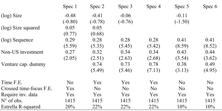
Table 3
Results in Table 3 show that, as anticipated, probability of being in-sample increases with both fund sequence and fraction of non-US investments. In-sample funds are also more likely to be venture capital funds. Being in-sample, however, is not related to fund size. Finally, there is little variation across years, i.e. including time fixed effects has a minor impact on results.
3. Performance measure corrections
In this section, we operate three corrections to the standard performance estimate. We first change the weights of individual fund’s performance in our aggregate estimate. Second, we assess the extent of sample selection bias and propose a correction. We operate in three steps: i) we investigate whether out-of-sample funds perform differently than in-sample funds based on a standard investment-based measure of performance (exit success); (ii) we estimate the relationship between cash-flow based performance measure (PI) and exit success in order to extrapolate the performance of out-of-sample funds and (iii) we correct the overall performance estimate for a potential sample selection bias. The third and final correction to the standard performance estimate consists in writing-off residual values after verification that they mostly correspond to living-deal investments.
A. Value-invested weighting
As seen in sub-section 2.B.2, it is standard practice to weight each fund by the total capital committed. However, the value invested differs from total capital committed as funds do not invest all capital upfront and vary in the speed at which they call capital (Ljungqvist and Richardson, 2003). If poorly performing funds invest more slowly, then capital-committed-weighted performance is downward biased (and vice versa). Another consequence is that the capital-committed-weighted PI of all the funds raised in a given year differs from the PI obtained by an investor who would have bought all the funds raised in that year. This is an undesirable feature as the purpose of value weighting is to assess the performance of the representative investor in a given year. In contrast, when we weight by the present value of the stream of
investments (‘value invested’), the PI of the sum of all fund cash flows is the same as the average PI in each vintage year.
Table 4
We thus weight fund performance by the ‘value invested’ from now on. The base date for the computation of the present value is the beginning of the fund’s vintage year. The consequence of such a change can be seen in Table 4. It is often relatively minor. In terms of overall average performance, it decreases the average PI from 1.01 (capital-committed weighted) to 0.99; the issue of performance aggregation will be further discussed below (section 4).
B. Correction for sample selection bias B.1. Performance and sample inclusion
In the literature, exit success is frequently used as a proxy for fund performance. Certain researchers use the fraction of investments exited via an IPO as a proxy for performance (e.g. Sorensen, 2006) while other researchers use the fraction of investments exited via either IPO or M&A as a proxy for performance (e.g. Hochberg, Ljungqvist and Lu, 2005). The widely held belief is that exit success and performance are highly related. As exit success is available for both in-sample funds and out-of-sample funds, we use this measure to document whether performance differs between the two samples.
Table 5
Table 5 reports the results from several ‘multiple regression’ specifications of exit success on fund characteristics (size, size-squared, sequence, fraction of non-US investments, venture-capital dummy variable) and on a dummy variable that takes the value 1 if the fund is in the cash-flow dataset, and 0 otherwise. This dummy variable is both highly statistically and economically significant. According to the baseline specification (Spec 1), a fund in the cash-flow dataset is expected to have an additional 6% of invested capital that is exited via either M&A or IPO. When using only fraction of exits via IPO, this is 3%. To put these figures into perspective, one can compare with the results in Hochberg, Ljungqvist and Lu (2005). The authors find that “the economic magnitude of this effect [network quality of GPs] is meaningful…a one-standard-deviation increase in network centrality increases exit rates by around two percentage points from the 34.2% sample average. Using limited data on fund IRRs disclosed following recent Freedom
of Information Act lawsuits, we estimate that this is roughly equivalent to a two percentage point increase in fund IRR from the 15% average IRR.”
B.2. Relationship between cash-flow based performance and exit success
The above result provides a first robust indication that out-of-sample funds are less successful than in-sample funds. Naturally, we need to verify whether there is indeed a tight relationship between exit success and cash-flow based fund performance, as assumed in the literature. Our data offer us this unique opportunity for the 618 in-sample funds for which both investment data and cash-flow data are available.
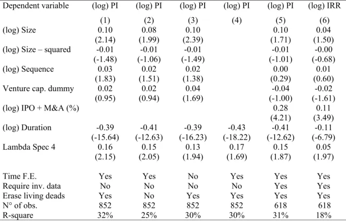
Table 6
In Table 6 - Panel A, we show several specifications with cash-flow based performance (log(1+PI)) as a dependent variable and exit success (log(1+fraction of investments that exit via either an IPO or an M&A)) as one of the explanatory variables. We add ‘1’ to both exit success and PI because each variable can take the value ‘0’. We start with all fund characteristics and with time fixed effects as control variables. We also separately estimate the effect of the exit success for venture capital funds and buyout funds. To measure performance, we also use the natural logarithm of (1+IRR) in two specifications (Specs 7 and 8) for illustration purposes. Finally, as in-sample funds are effectively liquidated, we either measure performance after writing off residual values or after converting the last residual value in a cash inflow of the same amount at that date (see sub-section 2.B.2).
We find that the relationship between cash-flow based performance and exit success is highly statistically significant in each specification. As we expressed both variables in log, the coefficient can be viewed as an elasticity. We find that a 1% increase in (1+) the fraction of successful exits entails a 0.29% increase in (1+PI), in the specification with highest adjusted R-square (spec. 3). Hence, if we have a PI of 0.90 for an exit success of 40%, then an increase in exit success to 45% would increase PI by 0.02 (i.e. about one standard deviation). In terms of IRR, if we have an IRR of 14% for an exit success of 40%, then an increase in exit success to 45% would increase IRR to 14.44%.
We also find that the relationship between cash-flow based performance and exit success is lower for venture capital funds but not statistically significantly so. The squared of fund size,
fund sequence, and fraction of non-US investments are found not to be significantly related to performance. The only significant variables are fund size and exit success.
Of interest, we find that if we redefine exit success as only the fraction of investments that exit via an IPO as is sometimes the case in the literature, the relationship between exit success and performance is weaker. Consequently, this result shows that it is likely better to count both M&A exits and IPO exits as successful exits as done in Hochberg, Ljungqvist and Lu (2005).
As the above relationship is based on a subset of funds, we need to verify that the relationship between cash-flow based performance and investment-exit based performance is not different for this subset of funds (compared to the universe). In other words, we should verify that taking into account the fact that our sample is selected does not bias our estimates. In Table 6 – Panel B, we show various so-called Heckit regressions (see Greene, 2003), which consists in adding the inverse of Mill’s ratio (denoted lambda) to the main specifications reported in Table 6 – Panel A. Mill’s ratio is related to the probability of a fund being in-sample given its characteristics and it is derived from the Probit model shown in Table 3; we show results using either specification 4 or 6 in Table 3 as they are respectively the one with highest Estrella R-square and most parsimonious. We find no significant effect of either lambda in any specifications. This indicates that the relationship between cash-flow based performance and investment-exit based performance is likely to be consistently estimated as far as sample selection issues are concerned. This is not surprising as sample selection considerations should not, a priori, affect the appropriateness of using exit success as a proxy for performance.
B.3. Performance extrapolation
From the above analysis, one can conclude that out-of-sample funds have a significantly lower performance than in-sample funds. A question of interest is to quantify the performance spread between in-sample funds and out-of-sample funds. In the analysis above, we have estimated the triplet (a,b,c) in the Equation (1) below. We also have estimated specifications that take into account that the dependent variable is observed only for certain funds (Equation (2)):
(1) ln(1+PI)=a+b*ln(size)+c*Exit
(2) ln(1+PI)=a2 +b2*ln(size)+c2*Exit+ρ2*λin−sample
However, for the funds of interest, i.e. out-of-sample funds, Equation (2) becomes: (3) ln(1+PI)=a3 +b3*ln(size)+c3*Exit+ρ3*λout−sample
It is therefore not formally possible to use either equation (1) or equation (2) estimated coefficients to extrapolate the performance of out-of-sample funds. Nonetheless, we find above that the hypothesis ρ2 =0 cannot be rejected. We then argue that it is likely the case that the hypothesis ρ3 =0 cannot be rejected either. In other words, the fact that accounting for sample selection issues does not affect the validity of the investment-exit performance measure as a proxy for in-sample funds indicates that using this proxy for out-of-sample funds is likely equally valid. Consequently, we use Equation (1) to extrapolate the performance of out-of-sample funds given their characteristics. We need to bear in mind though that this is an approximation as, formally, we should use Equation (3).
Results are reported in Table 6 - Panel A (bottom lines). We find that out-of-sample funds have an expected PI between 0.11 and 0.14 lower than that of in-sample funds depending on the model specifications. This spread is statistically significant for each specification and is thus robust to (not) writing-off residual values, including time fixed-effects, and including different fund characteristics as control variables. For illustration purposes, we also run two specifications with IRR and find that expected IRR is between 1.86% and 2.02% less for out-of-sample than for in-sample funds. For the rest of the analysis, we select the specification with the highest adjusted R-square (spec 3) and the corresponding extrapolated PIs for out-of-sample funds. According to this specification, the out-of-sample average (value-weighted) PI is 0.12 below the in-sample (value-weighted) average PI, which is statistically significant with a t-stat of 3.11.
To conclude, we find significant evidence for the existence of a sample selection bias. Performance estimates based on funds for which cash flow information is available have thus to be considered significantly overstated. Interestingly, our results are consistent with an observation by Kaplan and Schoar (2005, p1796) about the fact that in-sample funds might have above-average performance:11 “One potential bias in our returns sample, therefore, is toward larger funds. We also over-sample first-time funds for buyouts [opposite for venture capital funds]. As we show later, larger funds tend to outperform smaller ones, potentially inducing an upward bias on the performance of funds for which we have returns. Also, first-time funds do not
11 Kaplan and Schoar (2005) observe certain characteristics of out-of-sample funds but do not correct performance
estimates for a potential bias. This is likely because their paper does not focus on performance but on flow-performance relationship and flow-performance persistence. They show that sample selection issues do not change these core results. Note also that unlike us, KS do not have data on exit success, and this is the key variable used here.
perform as well as higher sequence number funds. Therefore, our results for average returns should be interpreted with these potential biases in mind.”
C. Residual values
C.1 Performance relevance of residual values
Another potentially important determinant of performance estimates is the valuation of Residual Values (RVs). In-sample funds have been selected in a way that they can be considered ‘effectively’ liquidated given their age (>10years) and lack of activity over the last six quarters. We note that half of these 852 funds are officially liquidated and that, surprisingly, 462 funds made up of a few officially liquidated funds and most of the non-officially liquidated funds, still report some residual value. Their total weight in terms of either capital committed, value invested or number is about the same as the total weight of the 390 other funds. They report a total residual value that is 43% of total amount invested. Consequently the assumptions regarding the treatment of these residuals should have a significant effect.
In the literature, two different assumptions have been made. First, following common practice, Kaplan and Schoar (2005) treat the final residual value as a cash inflow of the same amount at the end of the sample time period. That is, RVs are implicitly assumed to be an unbiased assessment of the market value of a fund. Kaplan and Schoar (2005) claim that for liquidated funds and funds with six quarters of cash flow inactivity (which is how both their sample and our sample are defined) this assumption has a limited impact on performance. Second is to write them off as in Ljungqvist and Richardson (2003). This seems more reasonable a priori as funds that are more than ten years old (typical liquidation age) and have not shown any activity (no cash distribution, no investment no fee collection) for more than six quarters are unlikely to distribute substantial additional cash. In such a case, RVs are said to represent ‘living dead’ investments.
In Table 4 (Panels A and B), we show that writing-off RVs rather than treating them as correct have a large impact on performance as it decreases the average profitability index by 0.07. For example, the standard average performance estimate of 1.01 (see sub-section 2.B.2) becomes 0.94 after writing off residual values (Table 4).
C.2 Residual value dynamics
As shown above, choices regarding the treatment of residual values have a substantial impact on performance estimates, even for a sample of effectively liquidated funds like ours. In this sub-section, we investigate the evolution of the residual values over time in order to gain further insights in the appropriateness of writing them off.
Table 7
As mentioned above, there are 462 in-sample funds that report a positive residual value as of December 2003 (end of our time period); they represent 50% of the capital invested (in present value terms). We first classify these 462 funds into different categories as a function of: (i) the net change in RVs between December 1998 and December 2000; and, (ii) the net change in RVs between December 2000 and December 2003. This is to assess the stickiness of net RVs in boom and down markets.
To capture the effect of write-ups or write-downs of residual values, rather than that of investments or divestments, we adjust the changes in RVs by intermediate cash flows. That is, we define net change in RVs between T and T+1 as follows:
T T T T T T RV RV RV I D RV +1− = ~+1− ~ + −
Where RV~T+1 denotes the reported residual value at date T+1, IT and DT denotes respectively the
investments and distributions made between dates T and T+1. As new investments are reported at cost at the time they are made, RVT+1−RVT represents the change in accounting values for non-exited investments.
Table 7 reports the proportion of the 462 funds in each category. This is reported in terms of numbers, value invested and residual values. The largest category (cat. 1; 46% of the funds, 40% of total residual values) contains funds that have had no change in residual values in either period. We also see that they do not have any cash flow activity. This means that they have been inactive over at least the last five years. Even with RVs treated as correct, this large group of funds exhibit the lowest performance of all categories (PI=0.71 with RVs treated as correct, PI=0.58 otherwise).
The next two most important categories of funds are those that changed their RVs between 1998 and 2000, but not since then (cat. 2 and cat. 3). In addition, they show no cash flow activities since January 2001. They represent 17% of funds in number, 25% of the funds in value invested and 31% of total residual values. These funds also exhibit low performance even with
RVs treated as correct (0.87 for cat. 2 and 0.89 for cat. 3). Given their inactivity over at least the last three years (and maximum five years), the residual values reported by these funds also appear to us as highly likely to be ‘living deads’. Altogether, these funds (cats. 1, 2 and 3) thus represent 71% of the total reported RVs and 58% of the value invested by non fully liquidated funds. If we were to write-off only these obvious living deads, and treating all the other RVs as accurate, then we can deduct from Table 7 that the average PI would decrease by 0.05 (instead of 0.07 when all RVs are written-off).
Among the remainder funds, many RVs still appear ‘suspicious’. In particular, 57% of the RVs of these remainder funds is reported by funds with no cash flow activities over at least the last 3 years. In total, we observe that 88% of the RVs reported by our sample of mature funds emanates from funds with no cash flow activities over at least the last 3 years. To obtain this figure from Table 7, one should multiply column 7 (% of funds in RVs) by column 10 (% in cat. with no cash-flow – in RVs) and take the sum. If we were to write-off only the RVs of funds with no cash flow activities over the last three years, then the average PI would still decrease by more than 0.06 (instead of 0.07 when all RVs are written-off; non-tabulated result).
Determining which investment is a living-dead and thus to what extent accounting valuation is exaggerated (or conservative) is bound to be a subjective exercise. We argue that it is most reasonable to write-off all residual values but it is important to bear in mind that erasing only the most obvious and treating as correct the remaining ones would affect average performance only marginally as seen above.
Moreover, we notice that the more suspicious RVs look, the lower fund performance is (even if we compute performance assuming RVs are correct market values). This is an additional hint that RVs might be strategically set as a function of performance. Indeed, cat 1 contains funds that are most likely living deads (no change in RVs, no cash-flows for more than 5 years). The average performance in cat 1 is 0.71 (assuming RVs are correct). It is the lowest performance of all the categories. The next lowest average performance is cat. 9 with 0.82. These funds have increased their RVs in both 1999-2000 and 2001-2003, which in itself is surprising, but, in addition, 82% of these funds do not have any cash-flow activity over at least the last three years. That is, they increased their RVs in a bear market without doing any investments or divestments. Such Rvs are then bound to be suspicious. The next lowest average performances are cat. 2, 3 and 7 with 0.87, 0.89 and 0.88 respectively. These are funds that have changed their RVs in
1999-2000 and either have not changed it since then or have decreased them only marginally after increasing them (cat. 7). These Rvs are therefore also suspicious but somewhat less than for the two categories above (cat.1 and cat. 9). At the other end of the spectrum, cat. 5 contains funds with highest performance (average PI is a staggering 1.57) and these funds have increased their RVs in 1999-2000 and have decreased them by at least as much in 2001-2003, which seems logical. These funds are those with the probably the most reliable RVs and, at the same time, have the highest performance. These funds are, however, rare (5% of total value invested by non-fully liquidated funds).
To conclude, looking at the detail of the evolution of the residual values over time brings further support to our decision of writing final residual values off.
C.3 Stickiness of residual values
The analysis presented in Table 7 allows us to make another interesting observation. Funds in cat. 3, which represent 16% of the total RVs and 12% of value invested, have written up their residual value during boom years (1999-2000) but left them unchanged during the down years (2001-2003). We also find that only 44% of the funds that wrote up their RVs during boom years, subsequently wrote them down by at least as much (cat. 5 compared to cats. 3, 6 and 7). Hence certain funds adjust their RVs to market conditions but they represent only 0.05/0.22 = 23% in terms of value invested and 0.03/0.31 = 10% in terms of RVs. This shows that the bulk of residual values are stickier in down markets than in up markets. This fact has important implications. For example, private-equity fund risk estimates often assume that residual values reflect market values up to a lag. The computed factor loadings and alphas will then be biased (e.g. Jones and Rhodes-Kropf, 2003).
D. Final performance estimate
In section 2.B.2, we reported an ‘uncorrected’ average PI of in-sample funds of 1.01. In table 4 – Panel A, we see that changing the weighting scheme from capital committed to value invested reduces average PI by 0.02. In table 4 – Panel B, we see that writing-off residual values reduces PI by 0.07, and that including the projected PI for out-of-sample funds decreases the average PI by 0.05. Irrespective of the order in which these three corrections are being made, they jointly
decrease performance from an average PI of 1.01 to 0.87, which is is found to be statistically significantly below 1 (t-stat is 3.26; non-tabulated).
Because profitability indices might be difficult to interpret, we convert them into a more intuitive figure by computing corresponding ‘alphas’. We assume that fund returns are given by the CAPM up to a constant alpha. The objective of this paper is to compare the performance of funds to the S&P 500, which is analogous to assuming a beta of 1 and finding the alpha that would make funds fairly priced. Hence alpha is defined as the constant to be added to the realized S&P 500 returns to make PI equal 1. Average alpha for each vintage year is shown in Table 4, in both Panel B and Panel C. The correspondence between alpha and PI is linear when PI is close to 1 but is irregular when PI moves away from 1. This is illustrated in figure 2. We see that the relationship is PI = 4.5 * alpha + 1, when PI is close to one. The plot is for a truncated sample to show the relationship around PI = 1. If PI = 1 then, it can be shown theoretically that we have PI = duration * alpha + 1; with duration defined as in the bond literature and in this paper (the average time at which distributions are made minus average time at which investments are made). As the truncation interval increases, R-square decreases dramatically.
In table 4 – Panel B, we report an average yearly alpha of -3.83% after the three corrections. Interestingly, in Table 4 – Panel C, we see that performance differs between venture capital funds (average PI is 0.81) and buyout funds (average PI is 0.91). However, the average alphas are similar. Venture Capital funds have an average alpha of -2.9% and Buyout funds have an average alpha of -3%. As pointed out above, the correspondence between PI and alpha is close to perfectly linear when alpha is close to 0 (see Figure 2). However, as alpha increases in absolute value, the relationship with PI becomes flat. The case of buyout and venture capital performance here illustrates this case. They have similar alphas but different PIs. Note that PI is, in general, the most meaningful measure economically speaking.
4. Robustness checks and further analysis
We have provided evidence that previous accounts of private equity fund performance are overstated and that mature private equity funds substantially and significantly underperform the S&P 500 Index. To gain further confidence in our analysis we perform several robustness checks to assess the sensitivity of our findings to certain assumptions.
A. Different benchmarks
The above results are derived using the S&P 500 as a benchmark. In this sub-section, we use instead either the NASDAQ Index (since we have a majority of venture capital funds) or the CRSP-VW index which includes all stocks traded on NASDAQ, NYSE and AMEX. Results are not tabulated.
Using NASDAQ produces virtually identical results as above. Unadjusted average performance is 1.01, and the final performance after doing the three corrections is also 0.87, i.e. identical to that documented above with the S&P 500. In contrast, funds fare better when compared to the CRSP-VW market portfolio. The unadjusted average performance is 1.04 and it is 0.90 after the three corrections. We conclude that the choice of a benchmark influences the magnitude of the underperformance, but the finding of significant underperformance is robust.
B. Performance Aggregation Revisited B.1. Aggregation of PI
As argued in sub-section 3.A, it is more appropriate to value weight fund performance by the present value of fund’s investments rather than capital committed. As we pointed out such a choice has a small impact on overall average performance (change in PI of 0.02). Nonetheless, in Table 4 - Panel A, we note that such a change impacts average performance dramatically in certain vintage years. For instance, for the 99 funds raised in 1989, the capital-committed-weighted PI is 1.12 while the value-invested-capital-committed-weighted PI is 0.96.
B.2 Aggregation of IRRs
IRRs have been frequently used as performance measures for private equity funds and are more popular among practitioners than PI. In this sub-section, we illustrate how average IRRs can be misleading.
The aggregation of IRRs is biased if IRR and duration are correlated. Indeed, IRR is a per period return while the object of interest to the investor is total return, i.e. duration * IRR. If they are correlated then E(duration*IRR)≠E(duration)*E(IRR). To illustrate, assume that good performance (say 100% IRR) occurs over 2 years on average and bad performance (say -20%) occurs over 10 years on average and that good and bad performance have equal probability then expected performance is not 60%. Note that such an issue is irrelevant for the PI since it measures excess return.
We dig further by empirically testing the relation between fund performance and duration. To compute the duration of a fund, we proceed as in the fixed-income literature. We first compute the average month at which cash-flows are received where the weights are the present value of the related cash flow divided by the present value of all the cash flows. Similarly, we compute the average month when capital was paid. The difference between the two dates is the fund duration.
Table 8
In Table 8, we report results of OLS regressions for fund performance (corrected for heteroskedasticity and including time-fixed effects). The dependent variable is either log(1+PI) as PI can be 0 or log(1+IRR). The explanatory variables include duration and the fund characteristics known to be related to performance (fund size, fund size squared, fund sequence, venture capital dummy, exit success) and we control for potential sample selection bias. In each specification, duration is by far the most significant and robust explanatory variable (t-stats range from -10.7 to -15.6).12
Funds with longer duration perform worse, hence the average IRR is biased upward. One way to correct for this bias is to weight each IRR by the product of the present value of investment and duration [duration*PV(invested)]. Thus, we obtain a sort of IRR per year and per dollar invested. Doing so decreases the average IRR from 14.64% to 12.22%, a substantial 2.42% spread. For the vintage year 1985, the size weighted IRR is almost twice as large as the average IRR that is both time and present value weighted (22.86% versus 13.88%).
12 Note that this variable could not be used in the above analysis despite its strong relationship to performance
because it cannot be constructed for out-of-sample funds. Also, fund duration might be jointly determined with performance inducing an endogeneity problem. For the problem at hand, endogeneity is not an issue as what we want to show is that duration and performance are highly correlated after controlling for other determinants of performance.
The bias in average IRR depends on the dispersion of fund duration in the sample. In a sample comprised of individual investments, the bias is expected to be more severe. For instance, we look at a sample of 2,991 LBO investments with duration over one year and size over $1 million for which we know the performance.13 The average size-weighted IRR is a staggering 55% per year but if IRR is both time-weighted and value-weighted, the average is 27%. To conclude, aggregation choice has a dramatic impact on IRR and standard averages of IRRs are highly misleading in the private equity context.
C. Performance of recently raised funds
More money and more funds were raised between 1994 and 2000 than between 1980 and 1993. Though performance figures for these are not yet definitive, it is interesting to see how these recently-raised funds fared.
Using the sample of mature funds (i.e. those raised between 1980 and 1993) at different stages of their life, we can infer the expected performance of the new funds. The model used to forecast final performance of new funds is based on a regression with the final performance of mature funds as a dependent variable and their corresponding characteristics as explanatory variables. Specifically, two sets of explanatory variables are used. The first set contains time unvarying fund characteristics: the natural logarithm of fund size and its square, the natural logarithm of the sequence number of the fund within its family, and a venture capital dummy variable. A second set of explanatory variables includes the characteristics of funds either in their 3rd year, 4th year, etc. all the way up to their 9th year. These characteristics are the realized performance at that time (intermediate PI without residual values; e.g. in their 3rd year), the ratio of residual value to present value of investments at that time, and three cross terms of the ratio of residual value to present value of investments at that time with respectively: fund sequence, fund size and fund focus (dummy variable that is 1 if venture capital). These cross products aim to assess the extent to which larger funds, more mature fund families and venture capital funds differ in terms of the aggressiveness or conservativeness of their reports of residual value.
To forecast performance of funds raised in 1994 (resp. 1995,…,2000), we use the regression of final performance on (i) the first set of characteristics and (ii) the characteristics of
13 These data are proprietary and come from fund raising prospectuses that we have assembled and that likely
the mature funds in their 9th year (resp. 8th year,…,3rd year). Regressions are estimated
independently for each vintage year (1994 to 2000) and final performance of mature funds is computed after writing-off residual values.
Table 9
Results for two specifications are reported in Table 9. In the first specification the characteristics in the second set of explanatory variables are expressed in log, while in the second specification, they are not. For consistency, in the first specification, the dependent variable is also expressed in log and not in the second specification. The use of log may be more appropriate for statistical inference while, economically, the relationship between final performance and intermediate performance is in level:
(4) ) ( int invested PV RV PI
PIfinal = ermediate + , which holds if residual value (RV) is an unbiased measure of the market value of the fund.
Results in Table 9 - Panel A show that intermediate performance becomes more precise as time passes, which is natural. It may be more surprising, however, to note that intermediate performance is highly related to final performance as early as Year 3 (t-statistics above 15). A similar result is also found in Kaplan and Schoar (2005). In contrast, residual values are not strongly related to final performance, which confirms our previous remarks regarding their noisiness. Interestingly, residual values appear to be more informative for large funds. They are also more informative for more established fund families (with high sequence numbers), but only in early years. Finally, we note that the R-squares are high, varying from 34% to 92% as we move from the regression for Years 3 to 9.
The expected performance of funds raised between 1994 and 2000 is then deduced and reported in Table 9 - Panel B. We report the results of the extrapolation for both specification 1 and specification 2. The first striking observation is that the amount of capital raised by private equity funds that are present in the cash-flow dataset during these seven years (1994 to 2000) is immense at almost three times that raised from 1980 to 1993. The number of funds, however, is similar with 852 mature funds and 1,171 new funds.
If we weight by value invested and treat residual values as accurate, then average PI of new funds is 1.01 (compared to 0.99 for mature funds). If residual values are written off, the average PI is 0.42. For such young funds, writing off residual values is obviously unwarranted