Project Report
Datasets and protocol for the CLIVAR WGOMD
Coordinated Ocean-sea ice Reference Experiments
(COREs)
October 2012
ICPO Publication Series No. 184
CLIVAR is a component of the World Climate Research Programme (WCRP). WCRP is sponsored by
the World Meterorological Organisation, the International Council for Science and the
Intergovernmental Oceanographic Commission of UNESCO. The scientific planning and development
of CLIVAR is under the guidance of the JSC Scientific Steering Group for CLIVAR assisted by the
CLIVAR International Project Office. The Joint Scientific Committee (JSC) is the main body of
WMO-ICSU-IOC formulating overall WCRP scientific concepts.
Bibliographic Citation
INTERNATIONAL CLIVAR PROJECT OFFICE, 2013:
Variability of the American Monsoon Panel. International CLIVAR
Publication Series No.184 (not peer reviewed).
Datasets and protocol for the CLIVAR WGOMD
Coordinated Ocean-sea ice Reference Experiments
(COREs)
Stephen M. Griffies1, Michael Winton2, Bonnie Samuels3
NOAA/Geophysical Fluid Dynamics Laboratory Princeton, USA
Gokhan Danabasoglu4, Stephen Yeager5 National Center for Atmospheric Research (NCAR)
Boulder, USA Simon Marsland6
CSIRO Marine and Atmospheric Research Aspendale, Australia
Helge Drange7, Mats Bentsen8,
University of Bergen/Bjerknes Centre for Climate Research Bergen, Norway
Version prepared on October 23, 2012
Abstract
This document describes the datasets and protocol for running global ocean-ice cli-mate models according to the CLIVAR Working Group on Ocean Model Development (WGOMD) Coordinated Ocean-ice Reference Experiments (COREs).
Contents
1 Overview of the CORE dataset 2
1.1 Attributes of the CORE datasets . . . 3 1.2 Some details of the dataset for CORE-IAF.v2 . . . 3
1[email protected] 2[email protected] 3[email protected] 4[email protected] 5 [email protected] 6[email protected] 7[email protected] 8[email protected]
2 The CORE protocol and further details about the CORE datasets 4
2.1 The CORE protocol in brief . . . 4
2.2 Radiative heating . . . 5
2.3 The importance of using the NCAR bulk formulae . . . 6
2.4 Details of the surface salinity and water forcing . . . 6
2.5 River runoff . . . 8
2.6 Air density and sea level pressure . . . 10
2.7 Properly referenced meteorological data . . . 12
2.8 Same treatment of saltwater vapor pressure . . . 12
2.9 High frequency meteorological data . . . 12
2.10 Using ideal age and chlorofluorocarbons (CFCs) . . . 12
2.11 Two sample CORE-IAF experimental designs . . . 13
3 Closing comments 15 AppendixA: TheCOREdataset web pages 16 A1 Datasets 16 A2 Support code and documentation 17 A3 Releases of CORE-IAF.v2 18 A3.1 May 2008: Initial Release . . . 18
A3.2 July 2008: Bug Fix . . . 18
A3.3 June 2009 extended data . . . 19
A3.4 January 2010 extended data and re-synchronization with NCAR . . . 19
A3.5 February 2011: updates to SAT and runoff . . . 19
A3.6 October 2012: updates for years 2008 and 2009 . . . 19
A4 Future releases 19
1. Overview of the CORE dataset
This document describes the datasets and protocol for running global ocean-ice climate models according to the CLIVAR Working Group on Ocean Model Develop-ment (WGOMD) Coordinated Ocean-ice Reference ExperiDevelop-ments (CORE). The CLI-VAR WGOMD recommends using the Large and Yeager (2004, 2009) datasets for use in various model comparison efforts, such as that documented in Griffies et al. (2009). The input fields for the CORE datasets (the “raw” atmospheric data) are based on a mixture of NCEP reanalysis and satellite observations – the river runoff data are largely based on gauge records. Although there are many caveats (Griffies et al., 2009), the CORE datasets and CORE protocol provide a means for the global ocean climate modeling community to integrate ocean-ice models without a fully coupled at-mospheric General Circulation Model (GCM), and to make meaningful comparisons of the simulations made by different research groups. The approach builds from earlier efforts by R¨oske (2001) for a Pilot-Ocean Model Intercomparison Project (POMIP),
and by R¨oske (2006) who provided a dataset for a repeating annual cycle. There have been other datasets developed for running coupled ocean and sea ice models, such as Brodeau et al. (2010) used for the DRAKKAR project in Europe.
1.1. Attributes of the CORE datasets
In brief, the CORE.v1 and CORE.v2 datasets have the following attributes.
• The CORE data combines NCEP reanalysis with satellite data, with the details of the combination motivated by certain limitations of reanalysis.
• The Large and Yeager (2004) algorithms are used in Version 1 of the interannu-ally varying forcing (IAF) CORE.v1, spanning the years 1958-2004, as well as a normal year forcing (NYF) derived from the interannual forcing. We refer to these “corrected” datasets as CORE-IAF.v1 and CORE-NYF.v1.
• Large and Yeager (2009) updated their original algorithms for the interannual dataset 1948-20079, thus producing CORE-IAF.v2. A corresponding normal year dataset, CORE-NYF.v2, is derived using the new corrections but applied to the original (1984-2000) uncorrected NYF data files.
There are two ways to use the CORE datasets to force ocean-ice models.
– online calculation of corrections: At NCAR, the Large and Yeager cor-rections are applied to the uncorrected datasets during the runtime of a par-ticular ocean-ice simulation. This strategy is preferred when developing the correction algorithms.
– pre-calculation of corrections: At GFDL and CSIRO, corrections are
ap-plied to the uncorrected datasets to produce a corrected dataset, which is then used to integrate the ocean-ice models. Once a final suite of correc-tions has been derived, it is sensible to work with the corrected datasets. This is the approach utilized by most groups that do not use the flux cou-pler from NCAR.
• The datasets are documented and supported by NCAR, with extensive refinement as more data are gathered. GFDL supports the release of both the “raw” or uncorrected data, as well as the corrected data resulting from applications of the Large and Yeager (2004) and Large and Yeager (2009) modification algorithms. Future releases of this data can be expected as improvements are made to the data products and to our understanding of their biases.
1.2. Some details of the dataset for CORE-IAF.v2
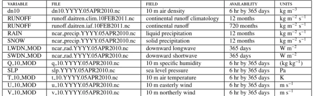
Table 1 details variable names, units, and temporal resolution of the CORE-IAF.v2 forcing fields suitable to force a CORE interannual run.
variable file field availability units
dn10 dn10.YYYY.05APR2010.nc 10 m air density 6 hr by 365 days kg m−3
RUNOFF runoff.daitren.clim.10FEB2011.nc continental runoffclimatology 12 months kg m−2s−1
RUNOFF runoff.daitren.iaf.10FEB2011.nc continental runoff 720 months kg m−2s−1
RAIN ncar precip.YYYY.05APR2010.nc liquid precipitation 12 months kg m−2s−1
SNOW ncar precip.YYYY.05APR2010.nc solid precipitation 12 months kg m−2s−1
LWDN MOD ncar rad.YYYY.05APR2010.nc downward longwave 365 days W m−2
SWDN MOD ncar rad.YYYY.05APR2010.nc downward shortwave 365 days W m−2
Q 10 MOD q 10.YYYY.05APR2010.nc 10 m specific humidity 6 hr by 365 days (kg kg−1)
SLP slp.YYYY.05APR2010.nc sea level pressure 6 hr by 365 days Pa T 10 MOD t 10.YYYY.05APR2010.nc 10 m air temperature 6 hr by 365 days K U 10 MOD u 10.YYYY.05APR2010.nc 10 m easterly wind 6 hr by 365 days m s−1
V 10 MOD v 10.YYYY.05APR2010.nc 10 m northerly wind 6 hr by 365 days m s−1
Table 1: Description of CORE-IAF.v2 forcing fields: column one gives the netcdf variable name; column two is the file name, with YYYY denoting each of the years 1948-2009 (river runoffis available only through year 2007); column three is the physical field; column four indicates the temporal resolution of the data; and the units are listed in column five. Note that: (1) continental runoffis for either a mean seasonal cycle or interannual varying data (Section 2.5.2); (2) precipitation fields are a climatological mean annual cycle prior to 1979; (3) the radiant (longwave and shortwave) fluxes are climatological mean annual cycles prior to 1984; (4) that the variable name annotation “ MOD” denotes modification of the NCEP/NCAR reanalysis fields according to the algorithms and methodology of Large and Yeager (2009); (5) all annual files for year 2005 carry the timestamp 06JUN2011 in line with a bug fix resulting in non-monotonic calendars; (6) and that the temperature files for 1997 through 2004 inclusive have timestamp 10FEB2011 in line with the update descibed in appendix A3.5.
1.2.1. Interannual forcing without leap-years
The interannual forcing fields in CORE-IAF.v1 and CORE-IAF.v2 do not contain leap-years. That is, each year has the same length of 365 days. This limitation may introduce some difficulties for those using the data for reanalysis efforts. However, the decision was made by NCAR to jettison the leap-years since many researchers find this to be more convenient given their software infrastructure.
1.2.2. Padding of years for the IAF
The IAF datasets for CORE-IAF.v1 and CORE-IAF.v2 are split into individual years with no overlap. The transition from one year to another is a detail that is left to the respective modellers, as it is a function of the modeller’s time interpolation code. At GFDL, the corrected IAF data are padded with a day on each side of the year boundary in order to smoothly time interpolate from one year to another.
Note that for CORE-IAF.v2, GFDL also provide the merged data files for all years 1948-2009. This single file should be usable by most time interpolation schemes for running a single realization of the full dataset.
2. The CORE protocol and further details about the CORE datasets
We now present some comments on particular aspects of using the CORE datasets for the purpose of running global ocean-sea ice climate models.
2.1. The CORE protocol in brief
The following summarizes the CORE protocol used for running global ocean-sea ice climate models. More details are provided both in Griffies et al. (2009) and later in
this section.
• The ocean models are initialized using the January-mean potential temperature and salinity from the Polar Science Center Hydrographic Climatology (PHC2; a blending of the Levitus and coauthors (1998) data set with modifications in the Arctic based on Steele et al. (2001)). More recent atlases may also be considered. As both the NYF and IAF simulations are run no less than 300 years, fine details of the initial conditions are not crucial. The sea ice models are generally begun with a state taken from an earlier simulation. The velocity fields typically start from rest.
• The surface heat fluxes are determined by the radiative fluxes from CORE, and turbulent fluxes computed based on the ocean state and CORE atmospheric state. Bulk formulae for the turbulent fluxes follow that used at NCAR. There is no restoring term applied to the surface temperature field.
• The surface salinity field is damped to a monthly climatology, with the climatol-ogy following Doney and Hecht (2002).
• For the NYF simulations, the repeating seasonal cycle river runoffdataset (Sec-tion 2.5) is used. For the IAF simula(Sec-tions, the interannually varying river dataset is used (Section 2.5).
• For the NYF simulations, the model is run for no less than 500 years, which has been found to be suitable for equilibrating the Atlantic meridional overturning circulation in the simulations documented by Griffies et al. (2009).
• For the interannually varying simulations, the model is run for no less than five repeating cycles of the forcing. Upon reaching the end of the year 2009, the forc-ing is returned to 1948. Analysis of the ocean fields durforc-ing the 5th cycle provides the basis for comparing to other simulations. Note that the 62-year repeat cycling introduces an unphysical jump in the forcing, with a notable warming trend over the 62 years of the atmospheric data. Nonetheless, no agreeable alternative has been proposed and tested.
2.2. Radiative heating
Radiative heating is provided from the shortwave and longwave datasets. The shortwave and longwave datasets representdownwellingradiation. Thenetshortwave radiation QSW net transferred into the ocean is a function of the albedo as shown by
equation (11) in Large and Yeager (2004). As discussed in Section 3.2 of Large and Yeager (2009), a latitudinally dependent albedo is used to compute the net shortwave in CORE-IAF.v2.
The net longwave radiation transferred into the ocean is given by the downwelling longwave radiation minus the loss of heat associated with re-radiation to the atmo-sphere as given by the Stefan-Boltzmann formulaeσT4as shown by equation (12) in
Large and Yeager (2004).
The CORE datasets provide a single shortwave radiation field. However, many ocean optics models make use of four different partitions of this shortwave field: visible
direct, visible diffuse, infrared direct, and infrared diffuse. NCAR recommends the following partition of downward shortwave components for the purpose of mimicing a more complete atmospheric radiation model:
Qvisible direct=0.28QSW net (1)
QIR direct=0.31QSW net (2)
Qvisible diffuse=0.24QSW net (3)
QIR diffuse=0.17QSW net (4)
2.3. The importance of using the NCAR bulk formulae
There is generally no restoring to surface temperature when using the CORE data set. Instead, turbulent heat fluxes are derived from the NCAR bulk formulae using the model SST and the 10 m atmospheric fields, and radiative heating is provided by shortwave and longwave fluxes.
Tests were conducted with the GFDL bulk formulae in CORE-NYF.v1 simula-tions. However, the fluxes produced from the two bulk formulae are quite distinct when running with observed SSTs. In particular, the wind stresses are larger with the GFDL formulation (which follows ECMWF) and the latent heat fluxes are larger with the NCAR formulation. The differences have been traced to differences in the neu-tral transfer coefficients (roughness lengths). As the forcing datasets developed using the NCAR bulk formulae, we recommend using the same (NCAR) bulk formulae for CORE experiments.
We originally went into the NCAR/GFDL comparison thinking that the bulk for-mulae differences should lead to minor differences in the fluxes. However, the GFDL formulae are somewhat different to NCAR’s. The resulting flux differences were too large to ignore, with the goal being to run the models with the same forcing when the SSTs were the same.
2.4. Details of the surface salinity and water forcing
The treatment of surface salt and/or water fluxes is the most problematic element in the CORE protocol. Many issues were raised in Griffies et al. (2009), and we sumarize these issues here.
2.4.1. Frozen and liquid precipitation
The uncorrected or raw precipitation file contains only liquid precipitation. How-ever, the corrected file ncar precip.YYYY.05APR2010.nc (see Table 1) contains both liquid and solid precipitation. The solid precipitation (SNOW) is determined during the correction algorithm by the air temperature; if less than freezing, then the precipitation is assumed to be snow.
2.4.2. Regarding the use of surface salt fluxes versus water fluxes
An ocean model that allows for the use of real water fluxes transferred across the ocean surface, such as naturally occurs for free surface formulations, has the option of applying the surface salt flux as a corresponding water flux. This approach, however,
is not encouraged, for the following reasons. First, the salt flux is an artifact of decou-pling the ocean model from the atmosphere. It thus should be seen as a mere means to keep the model’s overturning circulation from becoming overly unstable to allow for the simulation to be of use for studying mechanisms of climate variability. Second, by converting the salt flux to a fresh water flux, we are generally modifying the total water added to the ocean, unless some form of a global normalization is applied. Modifi-cations of water content, either local or global, induce a spurious barotropic flow, and will generally corrupt the use of the simulation for studying sea level variations.
2.4.3. Salinity restoring
As detailed in the Griffies et al. (2009) paper, different models may require diff er-ent restoring times for sea surface salinity to maintain a stable overturning circulation. Such remains part of the art, rather than the science, of ocean-ice climate modelling. It is therefore recommended that modellers garner experience via a selection of sim-ulation tests prior to settling on a particular means to handle the salinity boundary condition. The following summarizes some of the issues related to salinity restoring.
Relatively strong salinity restoring, analogous to the effective restoring of SSTs, may reduce model drift in some cases. However, salinity restoring has no physical ba-sis, and so it is desirable to use the weakest possible restoring. A weak restoring also has the benefit of allowing increased variability in the surface salinity and deep circu-lation. However, it can be associated with unphysically large variability and instability in the overturning circulation.
When the salinity restoring and effective temperature restoring timescales are very different, the experiment becomes analogous to a mixed boundary condition experi-ment. The ability of mixed boundary conditions to represent the adjustment of the ocean in the coupled system has been called into question. In particular, mixed bound-ary condition experiments with strong temperature restoring have been shown to be excessively susceptible to the polar halocline catastrophe, in which a fresh cap devel-ops in high latitudes and shuts down overturning (Zhang et al., 1993).
The effective temperature restoring determined by numerically linearizing the CORE thermal boundary condition is quite strong, yielding piston velocities around 1-2 m day−1. The salinity restoring strength chosen for a comparison between NCAR and
GFDL simulations with the normal year forcing was two orders of magnitude smaller than this (50 m (4 yr)−1)). Under these boundary conditions, the various models
doc-umented in Griffies et al. (2009) behaved quite differently, with some groups favoring stronger restoring to stabilize the Atlantic overturning.
Here is a summary of some further points to keep in mind regarding salinity forcing.
• GFDL and CSIRO use a real water flux instead of a salt flux. The salinity restor-ing may be converted to a water flux, or may remain as a salt flux. In the original simulations documented in Griffies et al. (2009), the salinity restoring was con-verted to water flux. Recent experiments retain the salinity restoring as a salt flux. The preference for salt flux is simply to maintain diagnostic control over the total water budget arising from P-E+R, and to not have that budget confused with added water from restoring.
• To ensure that there is no accumulation of salt in the model arising from the salinity restoring, it is useful to remove the globally integrated salt content from the restoring field at each model time step. Alternatively, when running with real water fluxes, this normalization occurs so there is zero net water introduced to the ocean due to the implied salinity restoring.
• As the ocean SST will deviate from that used to balance the dataset’s water con-tent, there is no guarantee that the water will balance as the model integrates. Hence, in addition to removing the global mean salt/water associated with the restoring, we recommend removing the global mean evaporation minus precipi-tation minus river runoffthat results from the bulk formulae. Again, this normal-ization ensures that no water accumulates in the model, and the normalnormal-ization is applied at each model time step. An alternative is to apply a precipitation and runoffcorrection factor which is computed for each year based on the change of the global-mean salinity during that year. This factor is used to multiply the pre-cipitation and runofffluxes during the next year to partially balance evaporation.
• Some groups choose to eliminate surface salinity restoring at grid cells receiving river runoff, so to not counteract the freshening by the overly salty values found in the salinity restoring field used in CORE (Doney and Hecht, 2002). This approach is not recommended for those who widely spread the river runoff, such as that used by NCAR (see Figure 2).
2.5. River runoff
River runoffin Griffies et al. (2009) was based on an annual mean for each river basin. However, recent updates from NCAR provide far more options with river runoff forcing. Note that for either runoffdataset, we provide a remapping scheme which will take the river data and map it onto a new grid, so long as the new grid is logically rectangular (such as the tripolar grids used at GFDL and CSIRO).
2.5.1. Runoffin CORE Version 1
The river runoffdata in CORE.v1 has only a single time step as it represents annual mean runoff. This data has been spread out from the river mouths in a manner used by NCAR for their climate models. This approach is thought to account for some unresolved mixing that occurs at river mouths in nature.
2.5.2. Runoffin CORE Version 2
Two options for CORE.v2 river runoffare now available which differ substantially from what was used in CORE.v1. These are a 12-month climatology
runoff.daitren.10202010.clim.nc
and a 720-month interannual dataset spanning 1948-200710
runoff.daitren.10202010.iaf.nc.
In both datasets, river discharge (in units of kg s−1 m−2) is provided at discrete river
mouth locations on a 1◦×1◦global grid. The CORE.v2 files are similar to the distribu-tions put together by Aiguo Dai and Kevin Trenberth in Dai and Trenberth (2002) and Dai et al. (2009), which are distibuted publically at
http://www.cgd.ucar.edu/cas/catalog/surface/dai−runoff/index.html
However, discrepancies identified in these distributions led to the generation of a mod-ified dataset (Dai, personal communication 2010), which extend the interannual data and ensure compatibility between the 12-month climatological data and the interannual data. We use this newest (October 2010) product from Aiguo Dai for CORE.v2.
Dai provided a runoffdataset from October 1947 through December 2006, and he offered the following comments.
There are missing data for many rivers since Oct 2004 and these gaps were infilled with latest 5yr mean values (i.e., Oct 1999-Sep 2004) for each month. These are scaled discharge that includes the contribution from unmonitored areas. The new data file was computed from com-plete records infilled with Community Land Model version 3 (CLM3)-simulated (through regression) flow for missing data gaps as discussed in Dai et al. (2009). Just to be clear, these discharge data were mainly based on actual measurements of river flow rates at the farthest downstream sta-tions, with small data gaps being infilled with CLM3-simulated flow rates (forced with observed precip etc) through regression, and scaled to repre-sent the flow rates at river mouths, and further scaled to include contribu-tions from drainage areas not monitored by the streamflow gauges.
These data were used to construct runoff.daitren.10202010.iaf.nc, with the 2007 monthly values filled with 5 year average values (from Oct 1999-Sep 2004). Further-more, a time-invariant distribution of runoffalong the coast of Antarctica was included. Antarctic runoffis estimated to be 73000000 kg s−1(0.073 Sv) based on P-E balance
(Bill Large, personal communication). This runoff is distributed as a uniform flux along the coastal points around the Antarctic continent (coastal points determined from ETOPO bathymetry on the 1◦×1◦grid). It enters the ocean as a liquid, so there is no prescribed calving land ice.
The 12-month climatology is the long-term mean monthly average discharge based on the interannual data computed over years October 1950 through September 1999. It also includes the time-invariant Antarctic runoff. The globally-summed annual mean river runofffrom this file is:
• Global=1.217 Sv (inclusive of Antarctica)
• Antarctica=0.073 Sv
We note that the new global value is somewhat lower than the published value from Dai et al. (2009).
2.5.3. Inserting river runoffinto the ocean
Version 1 of CORE, based on Large and Yeager (2004), employed a single annual mean river runoffthat was pre-spread according to the needs from NCAR modelling. The same approach was used by all groups in the Griffies et al. (2009) paper. Version 2 of CORE introduced the seasonally varying river runoffdataset from Dai et al. (2009), as well as an interannually varying version (see Figure 1). However, the Dai et al. (2009) river data is not pre-spread geographically. So the user must choose how to insert river water into the ocean model.
At NCAR, river runoffis spread substantially prior to applying it as a flux into the uppermost grid cell with a newer smoothing algorithm than was used in Large and Yeager (2004). The newer speading approach yields far less spreading than the original Large and Yeager (2004) approach. GFDL MOM simulations choose to apply two passes of a Laplacian (1-2-1) filter in the horizontal to spread the river runoff outward from the river insertion point. The latter results in a rather tiny spread. We illustrate the the three approaches in Figure 2. Notably, as detailed in Griffies et al. (2005), river runoffis inserted to the GFDL-MOM simulations over the upper four grid cells (roughly 40 m). This insertion provides a poor-man’s parameterization of tidal mixing near river mouths, and it may serve a similar purpose to the horizontal spreading applied by NCAR. In so doing, it helps to mix the fresh water over the uppermost part of the water column (throughout the upper four model grid cells), thus reducing the tendency for the simulation to produce a highly stratified fresh cap at the river mouths. 1950 1960 1970 1980 1990 2000 1.1 1.12 1.14 1.16 1.18 1.2 1.22 1.24 1.26 1.28 1.3
Global river runoff from Dai/Trenberth for COREïIAF
year
Sv
Figure 1: Time series for the annual mean global river runofffor the CORE-IAF simulations based on Dai et al. (2009).
2.6. Air density and sea level pressure
The subroutinencar ocean fluxes.f90computes the exchange coefficients for momentum, evaporation, and sensible heat according to the equations documented in Large and Yeager (2004) (see their Section 2.1). After computing the exchange coef-ficients, the model computes air-sea fluxes based on equations (4a)-(4d) in Large and
Figure 2: Shown here is the log of the river runoffmass fluxes (kg m−2s−1) used for the Large and Yeager
(2004) (top left); the 1988-2007 mean from Dai et al. (2009) as used in the CORE-IAF simulations using GFDL-MOM (top right); and the newer approach used at NCAR (lower center). Note the large spreading applied to the Large and Yeager (2004) river data, which is absent from the Dai et al. (2009) data. In fact, there is a slight amount of spreading applied according to a Laplacian operator applied by the ocean, but that spreading is very small relative to that used in the original Large and Yeager (2004) approach. The global net mass flux into the ocean from the Large and Yeager (2004) runoffis 1.24×10⁹kg s−1, whereas the
1988-2007 time mean from Dai et al. (2009) is 1.22×10⁹kg s−1.
Yeager (2004). This calculation requires the air density. There are three ways to get this density, each of which result in rather small differences.
• The air density at 10 m is provided in the uncorrected fields for version 2 of the IAF. Large and Yeager present no corrections to this field, so it can be used in CORE-IAF.v2.
• One may set air density to a constant 1.22kg m−3 (see Section 4.1 of Large and
Yeager (2004)).
• One may use the sea level pressure provided in the CORE datasets, and then use the ideal gas law to compute the air density.
The preferred method depends on the structure of the flux computation code that each modeler maintains. At GFDL, the sea level pressure and ideal gas law are used, and consequently no use of the 10 m air density dataset.
2.7. Properly referenced meteorological data
Models should use properly referenced meteorological data consistent with what the bulk formulae expect. Reanalysis meteorological data is commonly distributed at 2 m while oceanic turbulent transfer schemes often require 10 m data. For accuracy, it is essential that the data be re-referenced to 10 m. The re-referencing algorithm and the flux calculation algorithm are closely related. So, one should re-reference using a scheme that is compatible with the flux scheme.
2.8. Same treatment of saltwater vapor pressure
Models should use the same treatment of saltwater vapor pressure. The vapor pres-sure over seawater is about 2% less than that over fresh water. This difference is not negligible compared to the 20% subsaturation of marine air that drives evaporation. Consequently, the effect should be included in all models participating in a compari-son.
2.9. High frequency meteorological data
It is desirable to use high frequency meteorological data. A one month run of an AMIP model was used to explore the flux errors associated with averaged meteorologi-cal inputs. With daily winds, temperatures, and humidities, latent heat fluxes are under estimated broadly over the winter storm track band by some 10’s of W m−2. There was
also a smaller underestimate located in the summer storm track band. Experiments that refined the temporal resolution of the flux inputs individually showed that high frequency winds are most important for reducing the error but temperature and specific humidity frequency also contribute. When all inputs are given at 6 hourly frequency, the global RMS error is about 1 W m−2versus near 8 W m−2for daily inputs.
2.10. Using ideal age and chlorofluorocarbons (CFCs)
To help with assessing the models’ mixing processes, ventilation rates, deep water formation, and circulation characteristics under CORE forcing, we recommend that the simulations include ideal age tracer and CFCs.
2.10.1. Ideal age tracer
A number of groups participating in CMIP3 and CMIP5 have included ideal age tracer (Bryan et al., 2006; Gnanadesikan et al., 2007). This tracer (Thiele and Sarmiento, 1990; England, 1995) is set to zero in the model surface level/layer at each time step, and ages at 1 yr yr−1below. Furthermore, the tracer evolves according to the
advection-diffusion equation in the ocean interior just as a passive tracer. Ideal age is particularly useful for revealing surface-to-deep connections in regions such as the Southern Ocean where these connections have spatio-temporal variability. It can also be used to es-timate uptake of anthropogenic tracers such as carbon dioxide (Russell et al., 2006). Regions of low ventilation have the oldest waters while the younger waters indicate recent contact with the ocean surface. For a proper comparison of model ideal age distributions, we recommend that the ideal age be initialized with zero at the beginning of the 300-year simulations (corresponding to five forcing cycles).
2.10.2. CFCs
The CFC-11 and CFC-12 have been increasingly utilized in evaluating OGCMs, largely due to the following points:
• There is a good observational data base for comparison (the World Ocean Cir-culation Experiment, WOCE, upon which Global Ocean Data Analysis Project, GLODAP (Key et al., 2004) is largely based).
• There are well-known atmospheric concentrations that can be used to force the ocean.
• The CFCs are inert in the ocean.
The surface concentrations of CFC-12 and CFC-11 are available starting from 1931 and 1938, respectively. The associated fluxes should be calculated following the Ocean Carbon Model Intercomparison Project (OCMIP-2) protocols (Dutay et al., 2002). However, instead of the protocol specified fields, the CORE data sets should be used in the flux equations.
There is a mismatch between the CFC and CORE data start dates. At NCAR, the following approach is used. Recall that the CORE-IAF protocol calls for five forcing cycles, i.e., a 300-year simulation. The CFC-12 and CFC-11 surface fluxes are then introduced at the beginning of model years 224 and 231, respectively, in the fourth forcing cycle. Both CFCs are initialized with zero. These model years correspond to calendar years 1991 and 1998, respectively, for the surface fluxes of heat, salt, and momentum in the IAF cycle, while they correspond to calendar year 1931 for CFC-12 and calendar year 1938 for CFC-11 surface fluxes. However, by the beginning of the fifth cycle corresponding to model year 241 and calendar year 1948, all surface fluxes become synchronous, i.e., the calendar years for the atmospheric data used in all surface flux calculations are the same during the fifth cycle.
Another option is to simply introduce both CFCs at the beginning of the fifth cycle, i.e., in year 1948. Because CFC concentrations are rather small during the years before 1948, this approach is sensible.
2.11. Two sample CORE-IAF experimental designs
We present here two examples of how groups have made use of the CORE-IAF forcing.
2.11.1. CORE-IAF experimental design from Bergen
The following procedure is based on experience from the modeling group in Bergen, Norway, with emphasis of the North Atlantic subpolar gyre. We caveat the following discussions by noting that different model systems may respond differently. Further-more, some scientific problems may require longer spin-up than the five cycles recom-mended here (e.g., the marine cycling of carbon). Conversely, certain problems may require less cycles. Nonetheless, the following procedure is offered as an example of what other groups may choose to follow.
• Initialise the model based on climatological temperature and salinity fields, for instance from the World Ocean Atlas
http://www.nodc.noaa.gov/OC5/WOA05/pr woa05.html
and/or the Polar Science Center Hydrographic Climatology version 3.0 (PHC3.0)
http://psc.apl.washington.edu/POLES/PHC/Paper98.html
The ocean velocity is set to zero and there is a 2 m thick sea ice cover with extent according to climatology, for instance see
http://nsidc.org/data/seaice index.
• Spin up the model with daily varying reanalysis fields from CORE-IAF forcing until a quasi-steady solution is obtained. Experience indicates that for studies of the upper ocean, typically at least N=4 to N=6 cycles (240-360 years) are required. Each cycle past the initial one is initialized by the ocean state at the end of the previous cycle.
• During the spin-up phase, apply a relaxation of sea surface salinity (SSS) with a relaxation time scale of 30 days for a 50 m thick mixed layer, linearly decreasing with thicker mixed layers. No relaxation of surface temperature is applied, since the heat fluxes are computed from the bulk formulae. Additionally, there is no relaxation of sub-surface waters nor under sea ice. Continental runoffis included by adding freshwater into the appropriate coastal grid cells.
• Importantly, the mismatch between model and climatological sea surface salin-ity,∆(S S S), is limited to
|∆(S S S)|<0.5 ppt (5)
in the computation of the surface salinity relaxation. This limit avoids extreme relaxation fluxes that may occur, for example, in the vicinity of the western boundary currents that are generally not realistically represented in coarse OGCMs. If too much fresh water is added due to large biases in the western boundary cur-rent, then this potentially large amount of fresh water will be transported pole-ward, which will spuriously weaken the Atlantic overturning circulation. A sum-mary of this unstable feedback is given in Griffies et al. (2009).
• If focusing on quantities such as the Atlantic overturning, then one should gauge the degree of quasi-stationarity by examining the behaviour of the overturning. Additionally, time series of temperature and salinity as a function of depth may be used to determine suitability of the spin-up for studies being considered.
• When a quasi-steady solution is obtained after N cycles, the restoring surface salinity flux is stored on the horizontal model grid, averaged over cycle N+1, and saved with either weekly or daily temporal resolution.
• The production run starts with cycle N+2. Now the diagnosed, weekly or daily averaged (but inter-annually invariant) salinity flux from cycle N+1 is applied. In addition, the conventional surface salinity relaxation is applied, but with the relaxation time reduced by an order of magnitude; e.g., to 360 or 720 days for a 50 m thick upper ocean.
• It is the cycle N+2 that is used to focus analysis on the particular feature of interest.
Tests at GFDL indicates that the use of a diagnosed flux for the N+2 cycle can lead to rapid drift in the Southern Ocean. It is for this reason that most groups having used the CORE-IAF forcing do not choose the approach described above, preferring to maintain the same salinity restoring for all cycles.
2.11.2. CORE-IAF experimental design from NCAR
At NCAR, the ocean model is initialized using the January-mean potential tem-perature and salinity from the PHC2 climatology (a blending of Levitus and coauthors (1998) and Steele et al. (2001) data sets) and zero velocity. The sea-ice model is ini-tialized with a state taken from a preliminary ocean-ice coupled simulation.
A weak salinity restoring is applied globally using a 4-year time scale over 50m, including under ice covered regions, but excluding disconnected enclosed marginal seas (e.g., Black Sea). The global-mean of this restoring flux is subtracted every time step so that it does not impact the salinity budget. The salinity restoring data set is based on the PHC2 monthly-mean climatology and includes the salinity enhancements along the Antarctic coast described in Doney and Hecht (2002). There are no imposed limits in these salinity restoring fluxes. A global precipitation correction factor is computed for each year based on the change of the global-mean salinity during that year. This factor is used to multiply the precipitation and runofffluxes during the next year to partially balance evaporation. The precipitation correction factor in practice is of little consequence to the simulation.
In the disconnected marginal seas (e.g., Black Sea), strong restoring (25 days over 50 m) to PHC2 monthly climatology is applied for both potential temperature and salinity as these regions are not connected to active oceans in any way; i.e., their states do not feedback onto active oceans.
3. Closing comments
The CLIVAR WGOMD met in Venice, Italy during 11-13 January 2012. A major effort arose to coordinate simulations from about 12 models using the CORE.v2-IAF forcing and the protocol in Section 2.1. Analysis of the 5th cycle from these groups will ensue during 2012, with the aim of writing a suite of comparison papers. These notes will be updated as progress is made with the CORE-IAF comparison.
Acknowledgements
The CORE project would not exist without the efforts and leadership of Bill Large, whose continued contributions to this project are greatly appreciated. Numerous oth-ers within the growing community of CORE usoth-ers have greatly assisted in testing the CORE datasets and provided important feedback when problems were found.
Appendix A: The CORE dataset web pages
This appendix summarizes the material found on the CORE web pages. Version one of the dataset, CORE.v1, is based on Large and Yeager (2004), and it is available at
http://data1.gfdl.noaa.gov/nomads/forms/mom4/COREv1.html
This dataset has been updated by Large and Yeager (2009), which is known as the version 2 dataset, CORE.v2. This updated dataset is available at
http://data1.gfdl.noaa.gov/nomads/forms/mom4/COREv2.html
A1. Datasets
The CORE dataset web pages contain the following datasets.
• Version 1 datasets
– Uncorrected Normal Year Forcing (unCNYF.v1)
– Uncorrected Interannual Forcing (unCIAF.v1)
– Corrected Normal Year Forcing (CORE-NYF.v1)
– Corrected Interannual Forcing (CORE-IAF.v1)
• Version 2 datasets
– Uncorrected Normal Year Forcing (same as Version 1 unCNYF.v1)
– Corrected Normal Year Forcing (CORE-NYF.v2)
– Uncorrected Interannual Forcing (unCIAF.v2)
– Corrected Interannual Forcing (CORE-IAF.v2)
Each of the above datasets contain the following fields on a spherical grid of 192 lon-gitude points and 94 latitude points (T62 atmospheric grid):
• river runoff(annual mean; and since Feb2011 a seasonal and interannual dataset; see Section 2.5.2)
• monthly varying liquid (rain) and solid (snow) precipitation (12 time steps per year)
• daily varying shortwave and longwave (365 time steps per year; no diurnal cycle and no leap years),
• six-hourly varying 10 m temperature, density, specific humidity, zonal velocity, meridional velocity, and sea level pressure (4×365 time steps per year; no leap years).
A2. Support code and documentation
Besides the present set of notes and the datasets, the CORE web page also contains the following files.
• Version 1 support files
– Large and Yeager (2004): This report details both the uncorrected and cor-rected data sets used to produce the forcing fields. In particular, it provides an atlas of the fluxes produced when using Reynolds SSTs and the NCAR bulk formula to compute fluxes from the atmospheric state.
– Griffies et al. (2009): (CORE NYFv1.pdf): This manuscript documents seven global ocean-ice models run with CORE-NYF.v1 for 500 years.
– The Fortran codeadvance.f90provided by NCAR corrects the raw data. This code may be of use for those who compute the data corrections as the model integrates.
– The Ferret codemake data.cshprovided by GFDL implements the algo-rithms fromadvance.f90in a Ferret script.
– The Fortran codencar ocean fluxes.f90provided by GFDL computes the NCAR exchange coefficients recommended for use in CORE.
– The sea surface salinity restoring filePHC2 salx.ncprovided by NCAR for use in computing a restoring salt or fresh water flux with CORE.
• Version 2 support files
– The Large and Yeager (2009) paper documents the CORE-IAF.v2.
– README COREv2is a README file for the release of CORE-v2.0 from NCAR.
– The Fortran codedatm physTN460.F90provided by NCAR corrects the raw data in the case that a user wishes to make the corrections during a run (online) rather than prior to the run.
– The NetCDF filetn460nyf.correction factors.T62.121007.nc pro-vides the correction factors that are applied to the uncorrected datasets if users wish to run withdatm physTN460.F90.
– The Ferret codemake data CIAFv2.2008 06 18.csh(updated July 2008 from the original file make data CIAFv2.2008 04 22.csh) represents the GFDL implementation in a Ferret script of algorithms from the NCAR filedatm physTN460.F90.
– The Fortran codencar ocean fluxes.f90provided by GFDL computes the NCAR exchange coefficients recommended for use in CORE. This is the same file as in the Version 1 release.
– The sea surface salinity restoring filePHC2 salx.ncprovided by NCAR for use in computing a restoring salt or fresh water flux with CORE. This is the same files as the Version 1 release.
– A unix shell scriptget COREv2 data.cshto download the forcing files.
– Feb 2011: for the update to the surface air temperature as per Nudds et al. (2010), a Ferret script is provided that covers years 1997 thru 2004:
make data CIAFv2 AirTemponly.csh.
GFDL provides both the uncorrected and corrected forcing fields for two reasons.
• The user may wish to run simulations as at NCAR whereby corrections are ap-plied to the uncorrected fields at runtime by usingadvance.f90for CORE.v1 or
datm physTN460.F90for CORE.v2. This procedure facilitates further refine-ment to the corrections without needing to generate a new “corrected” dataset.
• At GFDL, corrections are applied prior to runtime using the above Ferret script.
A3. Releases of CORE-IAF.v2
This section documents the releases of CORE-IAF.v2.
A3.1. May 2008: Initial Release
The initial release of CORE-IAF.v2 occurred near the end of May 2008.
A3.2. July 2008: Bug Fix
Soon after the first release, the following two problems were identified:
• The air temperature was about 20◦C−30◦C warmer around Antarctica than with the CORE-IAF.v1 release. This spurious result arose from a bug in the Ferret scriptmake data CIAFv2.cshused to implement the Large and Yeager correc-tions, where
let cfac=cos(atan(1)*8/1460-0.298)
should in fact read
let cfac=cos(atan(1)*8*l[g=t 10]/1460-0.298)
The bug also spuriously affected the precipitation field, since air temperature determines how precipitation is partitioned into liquid and solid.
• The netCDF data files in CORE-IAF.v2 had a time axis which could lead to prob-lems with runs over multiple years. Andrew Wittenberg at GFDL has provided a self-consistent time axis for the various data files in the 8 July 2008 release. The 8July2008 bug fix release of the CORE-IAF.v2 dataset has updated ALL of the datafiles.
A3.3. June 2009 extended data
In June 2009, the interannual dataset was extended from 1958 back to 1948 for Version 2 of the IAF. Because the calendar meta-information changed in the datafiles, from origin at 1958 to new origin at 1948, All of the data files were replaced for the IAF. The data did not change for the years 1958-2006, but the calendar did, with the new origin.
Note that in addition to providing each data file split into individual years, there is also a merged data file for each forcing field, containing all of the years 1948-2006.
A3.4. January 2010 extended data and re-synchronization with NCAR
Early 2010, an extra year of data was released (for year 2007). In addition, NCAR updated the full 60 years of uncorrected data. This new version of the uncorrected data has some differences from the previous releases, thus making the corrected data differ as well.
A3.5. February 2011: updates to SAT and runoff
In February 2011, some corrections were released to the surface air temperature for years 1997–2004, as identified by Nudds et al. (2010). A new river runoffdataset was also released, including a monthly climatology and interannual dataset. Details of the river runoffdataset are given in Section 2.5.
A3.6. October 2012: updates for years 2008 and 2009
In October 2012, years 2008 and 2009 forcing data has been provided for the in-terannual forcing for all fieldsexceptthe river runoff. No changes were made to the normal year forcing.
A4. Future releases
A frequent request from the research community is to keep the CORE forcing up-dated to the nearest year, or even nearest month, with realtime. Alas, such requests go unfulfilled given resource constraints on those supporting the data. Additionally, the datasets that form the basis for CORE are in some cases not released to the public on a realtime basis. It is for these reasons that CORE data will likely be updated at roughly a two year periodicity for the near future.
References
Brodeau, L., B. Barnier, A. Treguier, T. Penduff, and S. Gulev, 2010: An ERA40-based atmospheric forcing for global ocean circulation models.Ocean Modelling,
31, 88–104, doi:10.1016/j.ocemod.2009.10.005.
Bryan, F., G. Danabasoglu, P. Gent, and K. Lindsay, 2006: Changes in ocean ventila-tion during the 21st century in the ccsm3.Ocean Modelling,15, 141–156.
Dai, A., T. Qian, K. Trenberth, and J. Milliman, 2009: Changes in continental fresh-water discharge from 1948-2004.Journal of Climate,22, 2773–2791.
Dai, A. and K. Trenberth, 2002: Estimates of freshwater discharge from continents: latitudinal and seasonal variations.Journal of Hydrometeorology,3, 660–687. Doney, S. C. and M. W. Hecht, 2002: Antarctic bottom water formation and deep
water chlorofluorocarbon distributions in a global ocean climate model.Journal of
Physical Oceanography,32, 1642–1666.
Dutay, J.-C., et al., 2002: Evaluation of ocean model ventilation with cfc-11: compari-son of 13 global ocean models.Ocean Modelling,4, 89–120.
England, M. H., 1995: The age of water and ventilation timescales in a global ocean model.Journal of Physical Oceanography,25, 2756–2777.
Gnanadesikan, A., J. Russell, and F. Zeng, 2007: How does ocean ventilation change under global warming?Ocean Science,3, 43–53.
Griffies, S. M., et al., 2005: Formulation of an ocean model for global climate simula-tions.Ocean Science,1, 45–79.
Griffies, S. M., et al., 2009: Coordinated Ocean-ice Reference Experiments (COREs).
Ocean Modelling,26, 1–46, doi:10.1016/j.ocemod.2008.08.007.
Key, R., et al., 2004: A global ocean carbon climatology: results from GLODAP.
Global Biogeochemical Cycles,18, GB4031.
Large, W. and S. Yeager, 2004: Diurnal to decadal global forcing for ocean and sea-ice models: the data sets and flux climatologies. CGD Division of the National Center for Atmospheric Research, NCAR Technical Note: NCAR/TN-460+STR.
Large, W. G. and S. Yeager, 2009: The global climatology of an interannually vary-ing air-sea flux data set.Climate Dynamics,33, 341–364, doi:10.1007/ s00382-008-0441-3.
Levitus, S. and coauthors, 1998: Introduction. Vol. 1, World Ocean Database 1998. NOAA Atlas NESDIS 18, NOAA/NESDIS, U.S. Dept. of Commerce, Washington, D.C.
Nudds, S., F. Dupont, and I. Peterson, 2010: Errors in the NCEP/NCAR Reanalysis-1 air temperature data in the Arctic between 1997-2004 and a post-processing correc-tion.Canadian Technology Report on Hydrography and Ocean Science,266, vi+20. R¨oske, F., 2001: An atlas of surface fluxes based on the ECMWF reanalysis: A climato-logical dataset to force global ocean general circulation models. Max-Planck-Institut f¨ur Meteorologie, Report No. 323.
R¨oske, F., 2006: A global heat and freshwater forcing dataset for ocean models.Ocean
Russell, J., K. Dixon, A. Gnanadesikan, R. Stouffer, and J. Toggweiler, 2006: Southern ocean westerlies in a warming world: Propping open the door to the deep ocean.
Journal of Climate,19, 6381–6390.
Steele, M., R. Morfley, and W. Ermold, 2001: PHC: A global ocean hydrography with a high-quality Arctic Ocean.Journal of Climate,14, 2079–2087.
Thiele, G. and J. L. Sarmiento, 1990: Tracer dating and ocean ventilation.Journal of
Geophysical Research,95, 9377–9391.
Zhang, S., R. Greatbatch, and C. Lin, 1993: A re-examination of the polar halo-cline catastrophe and implications for coupled ocean-atmosphere models.Journal