Improved Evolutionary Algorithm Design for
the Project Scheduling Problem Based on
Runtime Analysis
Leandro L. Minku,
Member, IEEE,
Dirk Sudholt,
Member, IEEE,
and Xin Yao,
Fellow, IEEE
Abstract—Several variants of evolutionary algorithms (EAs) have been applied to solve the project scheduling problem (PSP), yet their performance highly depends on design choices for the EA. It is still unclear how and why different EAs perform differently. We present the first runtime analysis for the PSP, gaining insights into the performance of EAs on the PSP in general, and on specific instance classes that are easy or hard. Our theoretical analysis has practical implications – based on it, we derive an improved EA design. This includes normalising employees’ dedication for different tasks to ensure they are not working overtime; a fitness function that requires fewer pre-defined parameters and provides a clear gradient towards feasible solutions; and an improved representation and mutation operator. Both our theoretical and empirical results show that our design is very effective. Combining the use of normalisation to a population gave the best results in our experiments, and normalisation was a key component for the practical effectiveness of the new design. Not only does our paper offer a new and effective algorithm for the PSP, it also provides a rigorous theoretical analysis to explain the efficiency of the algorithm, especially for increasingly large projects.
Index Terms—Schedule and organizational issues, evolutionary algorithms, software project scheduling, software project management, search-based software engineering, runtime analysis.
!
1 INTRODUCTION
Software project scheduling is traditionally one of the major problems faced by software project man-agers [2]. It is a particularly demanding task [3] and, being a project planning task, is vital to many software engineering activities [4]. Its process involves several duties [3]: identify project activities; identify activity dependencies; estimate resources for activities; allo-cate people to activities; and create project charts. As explained by Sommerville [3], project scheduling “involves separating the total work involved in a project into separate activities and judging the time required to complete these activities. Usually, some of these activities are carried out in parallel. Project schedulers must coordinate these parallel activities and organise the work so that the workforce is used optimally.”
In this work, we concentrate on the problem of optimally allocating people (employees) to activities (tasks) using automated approaches. Similar to pre-vious work [5], [6], [7], we will refer to this prob-lem as the Project Scheduling Probprob-lem (PSP). Typical
Authors in alphabetical order. A preliminary version with parts of the results and weaker theoretical results appeared in [1].
• L. L. Minku and X. Yao are with CERCIA, The University of Birmingham, Birmingham B15 2TT, UK.
E-mails:{L.L.Minku,X.Yao}@cs.bham.ac.uk.
• D. Sudholt is with the Dept. of Computer Science, University of Sheffield, Sheffield S1 4DP, UK.
E-mail: d.sudholt@sheffield.ac.uk
objectives to be optimised when making allocations are to minimise the cost and completion time of the software project. When allocating employees to tasks, employees can divide their attention among several tasks at the same time in the PSP. This is often modelled by dedication values [6] (Chang et al. [5] call it commitment quotas) representing the percent-age of time an employee spends on a certain task. Employees have a maximum dedication, which must be respected to avoid overwork. The PSP also has other constraints. For instance, the team assigned to a certain task must have all the skills required for this task, and task precedence constraints among tasks must be respected. All these factors contribute to the difficulty of the PSP, making it more complex than classical scheduling problems.
The PSP is particularly challenging when the project is large. The space of possible allocations of employ-ees to tasks is enormous, and providing an optimal allocation of employees to tasks becomes a very dif-ficult task [4]. So, it is desirable to have automated methods to provide near optimal schedules that meet all constraints and can aid a software project manager in his/her decision of what schedule to adopt in order to minimise cost and completion time of the project. In addition, budget and schedule compression has become the norm in today’s software industry [8], [9], as a result of its intensified competitiveness due to movements such as globalization, outsourcing and open-source software [10], [11], [12], [13]. As software companies have to strive to get their jobs done faster Digital Object Indentifier 10.1109/TSE.2013.52 0098-5589/13/$31.00 © 2013 IEEE
for less money in order to succeed [8], automated scheduling tools that can provide insight into how to reduce cost and completion time become increasingly important [14]. The advantages of automated methods are:
• they help the software manager in producing schedules that meet all constraints;
• they provide a very useful insight into how to optimise objectives such as cost and completion time, as they may find solutions that no human has thought of; and
• they speed up the task of allocating employees to tasks, as they can generate schedules taking far less time than a human would if he/she had to plan the whole schedule from the beginning. With Search-Based Software Engineering as a grow-ing field in Software Engineergrow-ing [15], evolutionary algorithms (EAs) [16] have been used to solve the PSP. Evolutionary algorithms mimic the natural evolution of species, “evolving” a population of candidate so-lutions, i. e. project schedules. Different EAs were adopted for different variants of the PSP, e. g. [17], [5], [6], [18], [19]. This also includes multiobjective variants of this problem [20], [7], [4], [21] as well as approaches using cooperative coevolution [22]. A comprehensive survey of related work was presented in the work by Di Penta, Harman, and Antoniol [4].
In order for search-based software engineering to be applied in the real-world successfully, we need to un-derstand fundamentally what search algorithms can and cannot do. However, despite the existing research, it is still not well understood how design choices in EAs affect performance for the PSP, including what problem features make the PSP a challenging problem for EAs. This lack of understanding makes it hard to make appropriate design choices for EAs to solve the PSP, and it impedes the design of better EAs for this problem. Fundamental understanding of algorithms used in software engineering is essential to advance the science. Some progress was made in the well-known work by Alba and Chicano [6]. They presented an effective EA and a systematic empirical perfor-mance analysis of the impact of problem features on the performance of their EA.
Our work presents a novel perspective for design-ing EAs for the PSP, based on rigorous mathematical arguments. We use runtime analysis to gain insight into how EAs perform on illustrative instance classes. This sheds light on what instances are easy, and which ones are hard to solve for EAs. It also helps to make more informed design choices for the PSP. Based on that, we propose a new design that is shown to be very effective both theoretically and empirically. Our design is thoroughly analysed and shown to outper-form others considering several criteria that may in-fluence a software manager’s choice of PSP algorithm. Such an analysis is important to software engineering
in practice because applying an algorithm/tool with-out understanding its benefits/limitations can lead to wrong conclusions.
This paper is organised as follows. Section 2 briefly explains the full process of software project schedul-ing, and how the duty of allocating employees to tasks (PSP) is integrated into it. Section 3 presents a formal definition of the PSP investigated in this paper. Section 4 explains previous works on using search-based techniques for the PSP. Section 5 presents our search-based approach for solving the PSP. Section 6 presents a runtime analysis to gain insights into the performance of EAs on the PSP in general, and on specific problem instances that are easy or hard. This rigorous theoretical analysis explains the efficiency of our approach. Section 7 provides an experimental analysis to provide the software project manager with insight into what algorithm to chose for the PSP. It gives evidence demonstrating what algorithms are likely to behave better according to different evalu-ating criteria that may affect the project manager’s decision. Section 8 provides an additional discussion on the comparison of different approaches. Section 9 presents the conclusions and future work.
2 THE
FULL
SOFTWARE
PROJECT
SCHEDULING
PROCESS
As explained in section 1, the full software project scheduling process involves several duties [3]: iden-tify project tasks; ideniden-tify task dependencies; estimate resources for tasks; allocate employees to tasks; and create project charts. This paper investigates the duty of allocating employees to tasks, which is called PSP for briefness. This section explains how the PSP is integrated into the full process of software project scheduling.
The PSP uses several pieces of information, which are determined in the prior duties of identifying tasks, identifying task dependencies, and estimating resources for tasks (estimating the effort required for the task, e. g., in person-months). The identification of tasks and their dependencies is performed by the soft-ware manager, possibly with the help of the softsoft-ware architect. After that, the software manager provides an estimate of the effort required to complete each of these tasks. Models such as COCOMO 81 [23] can be used as support tools in predicting the required effort based on features such as the estimated software size, development type and several cost drivers, such as required reliability, size of database, etc. Several other methods to estimate software effort exist (e. g., [24], [25], [26], [27], [28]). Additionally, the PSP also uses information about the employees, e.g., which employees are available for the project, and what their salaries and skills are.
After these prior duties are completed, one can proceed to the duty of allocating employees to tasks
(PSP). This paper is concerned with the problem of allocating employees to tasks in such a way to minimise the cost and completion time of the soft-ware project. In order to use an algorithm to search for such good allocations, a method to estimate the cost and completion time of the project is necessary. Several cost and completion time estimation methods exist [29], [3], [23], [26]. A feature that is common to most of them is the use of the estimated required effort as one of the main ingredients to estimate cost and completion time. In order to guide the search towards good allocations, the method used by the PSP must consider not only the required efforts, but also the allocations of employees to tasks. Considering the allocations is very important for software projects, because its resources are mainly human resources [30]. In this paper, schedule-driven estimation [29] is used for that purpose.
After the allocation of employees to tasks is de-cided, project charts can be produced. For instance, Gantt charts can be created using information about the tasks and their dependencies, required efforts and allocations.
3 PROBLEM
FORMULATION
This section provides a formal definition of the PSP as an optimisation problem, based on existing work [6]. It consists of the following inputs:
• a set of employees e1, . . . , en with salaries
s1, . . . , sn, and sets of skills skill1, . . . ,skilln,
re-spectively,
• a set of tasks t1, . . . , tm with required
ef-forts eff1, . . . ,effm, and sets of required skills
req1, . . . ,reqm, respectively, and
• a task precedence graph (TPG) – a directed graph with tasks as nodes and task precedence as edges. The set of tasks and TPG can be referred to as the project to be scheduled. The goal is to assign employees to tasks in order to minimise the com-pletion time as well as the total cost for the project (i. e. salaries paid). Employees can work on several tasks simultaneously, as indicated by their dedication to certain tasks. The dedication is the fraction of their time devoted to a particular task. The completion time is the time the project is completed. It is computed with a simple iterative algorithm (described in detail as Algorithm 1 in Section 5.2) that takes into account the task precedence graph, the effort for each task, and the dedication for all employees.
The amount of dedication of an employee ei
to a task tj is determined by a value xi,j ∈ {0/k,1/k, . . . , k/k}, wherek∈Nreflects the granular-ity of the solution. Fork= 1we only have dedications 0 and 1. For, say,k= 10we havek+1 = 11dedications of0%,10%, . . . ,100%. Employees can only work on a tasktj if all employees working together have all the
skills to do the task. More formally, we require
reqj⊆
n i=1
{skilli|xi,j>0}. (1)
A maximum dedication for each employee was considered previously [6]. It reflects how much of a full-time job an employee is able to work. This can reflect both part-time jobs as well as the willingness to work overtime. Alternatively, one could introduce theproductivityof an employee as a general indicator of her/his performance. The productivity of a part-time employee could then be decreased accordingly. It would also be feasible to associate different pro-ductivities with each skill so as to reflect how good an employee is at using a particular skill. This was done, for instance, in [18]. However, for the sake of simplicity we leave these aspects for future work and consider that all employees have the same maximum dedication of 1.
4 PREVIOUS
WORK ON
SEARCH-BASED
TECHNIQUES TO THE
PSP
4.1 EAs for the PSPSearch-based techniques such as EAs [16] have been showing success in solving resource-constrained scheduling problems [31]. However, such resource-constrained scheduling problems do not present some features that are important in software projects, e. g., the fact that employees can divide their attention among different tasks at the same time.
The software engineering literature on PSP is more recent than the literature on resource-constraint scheduling problems. For instance, Chang et al. [5] proposed an EA for a problem formulation similar to that in section 3. One of the main differences is that they considered overwork as an extra objective to be minimised.
Alba and Chicano [6] used the problem formulation explained in section 2 and proposed an EA which will be referred to as the Genetic Algorithm (GA) in this paper. Under this formulation, employees cannot exceed their maximum total dedication to tasks given by the company’s policy, but any amount of overwork within the company’s rules is allowed. Later on, Luna et al.[7] investigated a similar problem formulation in a multi-objective scenario where cost and completion time were not combined into a single fitness function. Their work also introduced a repair operator to im-prove finding feasible solutions. These algorithms are explained in more detail in sections 4.2 and 4.3.
Di Penta et al. [4] formulated the PSP as the problem of assigning employees to teams and deciding on the order that work packages are selected to be processed in a queue system. The queue system is then used to assign work packages to teams. Different search-based techniques such as single and multi-objective
EAs were investigated. The objectives are to minimise completion time and/or fragmentation, rather than completion time and cost. Fragmentation is the total amount of idle person-months in the schedule, due to the precedence constraints of the work packages to be processed.
Chang et al. [19] introduced a time-line to break down a task into smaller components of time-sliced activities. In this way, tasks can be interrupted after they start, and employees do not necessarily need to work on a certain task from its beginning until its end. Several other features were also introduced, such as distinction between an employee and a contractor, dif-ferent rates of payment depending on whether there is overwork, different proficiencies of the skills, possibil-ity of training during the project, etc. The inclusion of all these features creates a problem formulation closer to reality, but it also introduces a large number of subjective input values required by the algorithm. It is unknown to what extent the solutions provided by the EA employed in their study are sensitive to the uncertainty of these inputs.
Other examples of EAs for the PSP include the work of Kapur et al. [18], multi-objective EAs [20], [21] and cooperative coevolution algorithms [22]. A comprehensive survey of related work was presented in the work by Di Penta, Harman, and Antoniol [4].
Despite all the existing research, it is still not well understood how design choices in EAs affect perfor-mance, including what problem features make the PSP hard for EAs. This lack of understanding im-pedes the design of better EAs. In our work, we first tackle this issue theoretically considering the problem formulation proposed by Alba and Chicano [6] due to its popularity. A new design is then proposed to overcome problems specific to the existing algorithms designed for this problem formulation. Other problem formulations can be considered as future work. 4.2 GA for the PSP
Alba and Chicano [6] proposed a GA where candidate solutions for the PSP are represented as a matrix of bi-nary values which encode the dedicationsxi,jfor each
employee ei and tasktj. The recombination operator
is a 2-D single point crossover, which randomly selects a row and a column and then swaps the elements in the upper left and in the lower right quadrant of the two parents. They used bit-flip mutation, binary tour-nament selection of two parents for recombination, and survival selection based on elitist replacement of the worst individual.
A candidate solution is considered infeasible if there is a task with no employee associated, or the skills constraint (eq. 1) is not satisfied, or there are employ-ees working overtime. Overtime can happen when tasks are executed in parallel, as the total dedication of employees in the candidate solution can exceed 1.
Based on that, the fitness function is defined as fol-lows:
f(x) =
1/q if the solution is feasible 1/(q+p) otherwise,
whereq=wcost·cost +wtime·time,
p=wpenal+wundt·undt +wreqsk·reqsk +wover·over,
and wcost, wtime, wpenal, wundt, wreqsk and wover are
pre-defined parameters,costandtimeare the cost and completion time of the solution, undtis the number of tasks with no employee associated, reqsk is the number of skills still required to perform all project tasks, andoveris the total amount of overwork time spent by all employees during the project.
Their fitness function penalises infeasible solutions, but whether or not it gives hints as to how to reach feasible solutions depends on the chosen values for several pre-defined parameters (wpenal, wundt, wreqsk
andwover). So, a wrong parameter choice could make
the algorithm unable to guide the search towards feasibility. Moreover, their experimental analysis re-veals that the overwork constraint can cause their GA to have very low hit rate in finding feasible solutions, i.e., the algorithm is unable to find feasible solutions in several occasions. This holds even for very simple instances where the skill constraints have been removed (every employee has all skills) and all employees have the same salary.
4.3 A Repair Mechanism
After the preliminary version of this paper [1] was prepared, we learned that Luna et al. [7] indepen-dently proposed a repair mechanism that facilitates the search for feasible schedules without overwork. Their repair mechanism considers the maximum total dedication of any employee at any point of time during the generated schedule:
M := max
i,τ {e
work
i (τ)}+ε
where ework
i (τ) is the total dedication of employee i
at time τ, and ε = 0.00001 is a small constant used to prevent floating point inaccuracies. If M >1 +ε, i. e., if there is overwork, dedications of all employees on all tasks are scaled down by dividing them byM. This implies that overwork is eliminated, but this is done at the expense of increasing the execution time of all tasks by a factor ofM.
In many settings this approach might be suboptimal as dedications are unnecessarily reduced during the periods of the schedule where there is no overwork, as long as there is overwork in at least some period of the project.
5 OUR
APPROACH
In order to overcome problems related to the hit rate and to improve solution quality, we propose an
improved design, which consists of two main points. The first one is to normalise employee’s dedications (section 5.1) in order to address the problem of over-work. It provides an alternative solution to the re-pair mechanism from [7], trying to reduce dedication values only where necessary, instead of reducing all dedication values across the board. The second one is to give a clear gradient for searching towards feasibility by introducing a new type of penalty in the evaluation of cost and completion time (section 5.2). This improved design can be used with different algorithms. Our experimental analysis (section 7) uses it with the (1+1) EA, RLS and Pop-EA as explained in section 5.3.
5.1 Normalising Dedications
We alleviate the problem of overwork and hence remove a crucial obstacle in the search process of EAs by using the following approach (normalisation): if at some point of time the total dedication of an employee ei across all active tasks is di > 1 then
her/his dedication for all tasks at this point of time is divided bydi. This reflects a very natural way of an
employee dividing her/his attention to several tasks. Note that we do not normalise “underwork”, i. e., total dedications less than 1. This would otherwise remove the possibility of balancing cost vs. completion time.
Normalisation allows for much more fine-grained schedules as employees can automatically re-scale their dedications as soon as tasks are finished or new tasks are started. For instance, assume there are two taskst1, t2suitable for employeee1under the problem
formulation explained in section 3. Assume also that the employee works on both tasks at overlapping time intervals and neither normalisation nor repair are used. Ifx1,1+x1,2>1, the employee works overtime
whenever she/he works on botht1andt2at the same
time. If x1,1+x1,2 ≤1, on the other hand, resources
are wasted when the employee works on a single task. So, regardless of the values forx1,1andx1,2, there will
always be overwork or resources wasted—unless both tasks start and finish at exactly the same time. Note that, depending onx1,1 andx1,2, there could be even
both resources wasted when the employee is working on a single task and overwork when working on both tasks at the same time (whenever x1,1 <1,x1,2 <1,
and x1,1+x1,2>1).
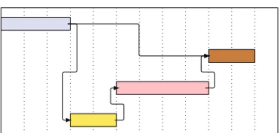
With normalisation the semantic of dedication val-ues is changed slightly. For any employee working on two or more tasks, equal dedication values mean that she/he should divide her/his attention equally among all tasks. Dedications 0.5 and 1 mean that she/he should devote twice as much time for the second task as for the first task. A smallest possible example is given in Figure 1. In this example, the schedule with neither normalisation nor repair is in-feasible. In the repaired schedule, the employee uses
100% 100% 50% 50% 50% 100% 50%
Fig. 1. Three Gantt diagrams, highlighting the dedica-tion of employee e1 working on two tasks (t1 and t2)
simultaneously with x1,1 = 1 and x1,2 = 1. Left: an
infeasible schedule with overwork. Middle: the same schedule after repair, without normalisation. Right: the same schedule with normalisation.
only 50% of her/his time to complete the first task. Normalisation, on the other hand, would decrease dedications of 100% towards 50% as long as two tasks are performed, and then it would automatically remove this scaling factor, so that the dedication of the first task goes back up to 100% after the other task is completed. We will come back to the comparison of normalisation and repair in section 8.
5.2 Evaluating Costs and Completion Time Algorithm 1 makes a schedule-driven estimation of cost and completion time by implicitly constructing a Gantt diagram as explained in the following. If the dedication matrix is the genotype during optimi-sation, the final schedule can be calledphenotype. The phenotype for any feasible genotype is constructed iteratively (lines 8–28), and is assessed by storing the
di,j-values from each iteration, along with the
corre-sponding time stamps. The algorithm checks which tasks can be active at the current point of time (line 9). The normalised dedication for all suitable employees is computed for all these tasks (line 15). Then we determine the earliest point of timetat which a task is finished (line 19). All finished tasks are being marked as finished (line 25), so that the next iteration can include new tasks, according to the task precedence graph. If there are tasks that have been started, but are not finished yet, their effort is updated to the remaining effort needed for completing them (line 23). This accounts for potentially piecewise evaluations of particular tasks. Along the way, all completion times and costs in all iterations are added up (lines 20-21). The total completion time and cost are the output when all tasks have been processed (line 29).
Before constructing the schedule, Algorithm 1 tests whether the genotype is infeasible in that not every task can be completed in finite time (lines 1-4). That is the case when the skills constraint (eq. 1) is not satis-fied. Note that this includes the case in which there is a task with no employee designated, as tasks with no employee associated can be seen as tasks lacking all the required skills. If the genotype is infeasible, the al-gorithm returns very high costs and completion times
Algorithm 1 Evaluate(cost,time,TPG) Output:(cost,time)
1: Let reqsk = 0.
2: for all taskstj do
3: reqsk = reqsk +|reqj\ni=1{skilli|xi,j>0}|.
4: end for 5: ifreqsk>0then 6: Output reqsk·2n i=1 m j=1 sieffj,reqsk·2k m j=1 effj ; stop. 7: end if 8: while TPG=∅ do
9: LetV be the set of all unfinished tasks without incoming edges inTPG.
10: ifV=∅ then
11: Output “Problem instance not solvable!” and stop.
12: end if
13: forall taskstj inV do
14: forall employees ei do
15: Letdi,j:= max1,xi,j
t∈Vxi,
.
16: end for
17: Compute the total dedicationdj :=ni=1di,j.
18: end for
19: Lett:= minj(effj/dj).
20: Letcost := cost +tni=1si
m j=1di,j.
21: Lettime := time +t.
22: forall taskstj inV do
23: Let effj := effj−t·dj.
24: ifeffj= 0 then
25: Marktj as finished and remove it and its
incident edges fromTPG.
26: end if
27: end for
28: end while
29: Output (cost,time) and stop.
(line 6):(reqsk·2ni=1mj=1sieffj,reqsk·2kmj=1effj),
wherereqskis the number of required skills missing. These values are chosen in such a way that any improvement in decreasing the number of missing skills results in a solution that has both lower costs and lower completion times:
Lemma 1: The output of Algorithm 1 is such that for every two solutionsx, y, if yhas fewer missing skills than x (including no missing skills) then cost(y) <
cost(x)and time(y)<time(x).
A proof of this lemma is given in the appendix. This implies that any decrease in the number of required skills missing strictly decreases both com-ponents through reqsk. When cost and completion times are used in any reasonable single- or multi-objective fitness function, this gives a clear gradient for search algorithms towards feasibility, without the need for pre-defined parameters to guide the search towards feasibility as done in previous work [6]. It
is also worth noting that this strategy deals both with solutions that are infeasible due to the skills constraint and due to tasks with no employee associated. An EA using it can have a very simple fitness function which does not need to treat these two types of infeasible solution separately as done in previous work [6]. 5.3 New EA Designs
When designing an EA, one needs to chose the encod-ing (internal representation of candidate solutions), mutation (operator to create a new candidate solution by modifying an existing one), crossover (optional operator to create new candidate solutions by com-bining existing ones), and fitness function (procedure to evaluate the quality of a candidate solution). This section presents our design, as well as the algorithms used in our study. For general knowledge on EAs, we refer the reader to [16].
5.3.1 Encoding and Mutation
A binary encoding was used previously [6] to rep-resent xi,j. This however means that the probability
of turning one numerical value into another by mu-tation depends on the binary encoding of these two values. As a result, some mutations (e. g., mutating 7/k 01112 towards 8/k 10002 flipping 4 bits) are
less likely than others (e. g., mutating 8/k 10002
towards9/k10012 flipping 1 bit).
We follow a different approach and work with a direct encoding of dedication values: the search space is{0/k, . . . , k/k}nm. Mutation is performed by changing each entry xi,j of the dedication matrix
with probability Pm = 1/(nm), independently from
other entries. Changing an entry xi,j means
replac-ing it by a value chosen uniformly at random from
{0/k,1/k, . . . , k/k}\{xi,j}. This implies that each new
value has the same chance of being created by mu-tation. Note that mutation has a chance of changing several dedication values at the same time, changing only a single entry, or not changing any entries at all.
5.3.2 Crossover
In this paper, the crossover operator uses two parent candidate solutions to create two offspring candidate solutions by selecting one of the following two strate-gies with an equal probability:
• For each employee, select its corresponding dedi-cations to tasks from one randomly chosen parent to compose the first child, and from the other parent to compose the second child. This can be seen as exchanging “rows” of employees’ dedi-cations if we visualise the valuesxi,j as a matrix
of employees by tasks.
• For each task, select its corresponding employees’ dedications from one randomly chosen parent to compose the first child, and from the other parent
to compose the second child. This can be seen as exchanging “columns” of dedications to tasks. The above is different from the crossover operator used before [6]. The reason is that their operator, which is a 2-D single point crossover, allows part of the dedications of an employee to tasks to be inherited by one child and the remaining part by the other child. So, if a solution is good because the dedications of a certain employee are well balanced for the problem instance, crossover can break this balance by mixing these dedications with dedications of another employee. An illustrative example of that in their algorithm is the fact that, even if the par-ents do not contain overwork, crossover could easily generate children with overwork. A similar problem could happen to the dedications of all employees to a certain task. Our crossover operator either exchanges full rows of employees’ dedications or full columns of dedications to tasks, in an attempt to avoid breaking balances that may be important for the solutions. As it is not known a priori whether the balance in terms of rows or columns is more important, our crossover gives 50 percent of chance for exchanging rows and 50 percent for columns.
5.3.3 Fitness Function
A very simple fitness function can be used based on Algorithm 1. The fitness function (to be minimised) used in our experimental analysis is f(x) = wcost ·
cost +wtime·time, where costand timeare obtained
from Algorithm 1. The only pre-defined parameters in this fitness function are the weights wcost and
wtime, which are used to adjust the desired relative
importance of cost and completion time. So, it is easier to configure than other fitness functions [6]. The runtime analysis is not restricted to this fitness function.
5.3.4 Algorithms
As our main goal is to introduce runtime analysis for the PSP, we follow many previous examples in this area [32], [33], [34], [35] and use one of the simplest EAs in our theoretical studies: the (1+1) EA. It is simple because it uses a “population” of just one individual and it does not use crossover. One genera-tion consists of mutagenera-tion, and then selecgenera-tion checks whether the mutation has found an improvement. Algorithm 2 describes the (1+1) EA for our search space, for minimising some fitness function f. The encoding, mutation and fitness function used in this paper are described in sections 5.3.1 to 5.3.3.
In practice, like all EAs, it will be stopped either after a certain amount of time has elapsed, or when a satisfactory solution has been found. For a theoretical analysis it is a common practice to consider an EA as an infinite process and to measure the expected time needed to find a global optimum. Note that
Algorithm 2(1+1) EA for project scheduling
1: Initialisex.
2: repeat
3: Create x by copyingx.
4: Apply mutation to x using probabilityPm.
5: iff(x)≤f(x)thenx:=x.
6: untilhappy
the expected number of components changed in one iteration equals 1. The (1+1) EA is a bare-bone version of EAs and captures their core working principles in a very clear fashion. It can also be a very effective EA, when considering the number of fitness evaluations as the performance measure. For well-known functions like ONEMAXand LEADINGONESthe (1+1) EA is the best EA that only uses mutation for variation [36].
We will also investigaterandomised local search (RLS). It differs from the (1+1) EA in that during mutation exactly one dedication value is changed. The entry is chosen uniformly at random. So, RLS can only make local steps, i. e., it can easily get stuck in a local optimum. The (1+1) EA has a global search operator, which allows larger jumps to be made, so that the (1+1) EA can, in principle, escape from any local optimum. However, large jumps are only made with a small probability.
From a theoretical perspective the (1+1) EA is harder to analyse than RLS. The reason is that a mutation changing multiple dedication values simul-taneously may have both beneficial and detrimental effects. The mutant will be accepted in the light of detrimental mutations if the combined effect of all changes on fitness is non-negative. There are situa-tions where a mutation is accepted, even though the mutant is “further away” from the optimum, in a sense that less dedication values coincide with the respective values in the global optimum.
In order to check whether improvements in solu-tion quality can be obtained by using a populasolu-tion, our experimental analysis also considers the (μ+λ) population-based EA (Pop-EA) presented in Algo-rithm 3. It differs from the (1+1) EA in that it main-tains a population of μ candidate solutions, rather than a single solution. At each generation, λparents are selected based on binary tournaments. Crossover is applied to each pair of parents with a pre-defined probabilityPc. Mutation is then applied to each child
as in the (1+1) EA. The mutation and crossover oper-ators used in this paper are explained in sections 5.3.1 and 5.3.2, respectively. An elitist approach that retains the bestμcandidate solutions among the parents and children is used to select candidate solutions that survive for the next generation.
A summary of these algorithms is presented in Table 1. This table also shows two other algorithms that will be used in section 7.
TABLE 1
Summary of the algorithms used in our study.
Algorithm Encoding Mutation Crossover Parent selection Survival selection Population size Normalisation (1+1) EA Direct Uniform – – Elitist 1 Yes RLS Direct Uniform – – Elitist 1 Yes
1 entry
Pop-EA Direct Uniform Rows/columns λbinary tournaments1 Elitist μ Yes
(1+1) EA no-norm Direct Uniform – – Elitist 1 No GA [6] Binary Bit-flip 2-D single point 2 binary tournaments1 Elitist μ No 1Number of tournaments per generation.
Algorithm 3 Pop-EA for project scheduling
1: Initialise populationP withμcandidate solutions.
2: repeat
3: Select λ parents from P using binary tourna-ment selection.
4: foreach pair of parentsx(1) andx(2) do
5: With probabilityPc, apply crossover between x(1) and x(2) to generate x(1) andx(2).
6: Otherwise, x(1)←x(1) and x(2)←x(2)
7: Apply mutation tox(1) andx(2) using
prob-abilityPm.
8: P ←P∪ {x(1), x(2)}.
9: end for
10: Select theμbest candidate solutions fromP to survive for the next generation, based on the fitness functionf.
11: until happy
6 RUNTIME
ANALYSIS
In the following, we estimate theoretically the optimi-sation time of the (1+1) EA and RLS, defined as the first generation in which a global optimum is found. The only assumption we make about the fitness functionf is that it isPareto-compliantin a strict sense: if x Pareto-dominates x (i. e., cost(x) ≤ cost(x)∧
time(x)≤time(x)) andxdoes not Pareto-dominatex
thenf(x)< f(x). That is, any improvement in one or both objectives also improves the fitnessf. This is the case, for instance, when the fitness is chosen as any weighted combination of cost and completion time, and our results are independent of the choice of these weights. In the special case where all employees have the same salary, the costs are always the same. Thenf
boils down to minimising the completion time; and as (1+1) EA and RLS only depend on the order of search points, and not on their absolute fitness values, we can then, without loss of generality, takef(x) = time(x).
For details about asymptotic notation (O,Ω,Θ) used in the following, we refer the reader to [37].
6.1 Optimal Completion Times
The two goals of minimising costs and completion time are often conflicting. We first look at the ex-treme case of minimising the completion time only. In every feasible solution for each task the team has
the required skills for the task. This also holds if more employees join in working on a task, regardless of their skills. The following theorem describes the optimal solutions to this special case.
Theorem 2: For every solvable PSP instance, the completion time is minimal if in the schedule all em-ployees always work full time. Then the completion time is1/n·mj=1effj.
If normalisation is used, a sufficient condition for minimality is that all dedication values are 1.
The proof of the first statement is straightforward as all employees will work full time until the project is completed. It is obvious that this minimises the completion time.
The second statement is not true without normalisa-tion, as the all-1s matrix will lead to massive overwork on almost all instances. Without normalisation, the difficulty for optimisation is to find the ideal balance between different tasks, while avoiding overwork. When normalisation is used, this difficulty disap-pears.
6.2 General Time Bounds
This section presents general time bounds for arbi-trary instances of the PSP and almost arbiarbi-trary EAs. The considerations herein are based on the progress EAs, and, specifically, local and global mutation op-erators, can make at the genotype level.
We first present a lower bound on the expected running time, in case the problem only allows for a single optimal solution. This lower bound indicates the least time we should allow for running an EA on the problem. In a more general sense, the analysis applies to the time for finding any fixed target point. Theorem 3: Consider a PSP instance with n em-ployees and m tasks, nm > 1, with a single global optimum (a fixed target) in the fitness function used. Consider an EA starting with a population of random solutions (of arbitrary size) and afterward creating new solutions from previously created ones by local or global mutations. The expected optimisation time (time to hit the target) of the EA, with or without normalisation, is at leastΩ(knmlog(nm)).
A formal proof is given in the appendix. In simple terms, the analysis shows that initially many dedica-tion entries will differ from their optimal values. In
order to find the global optimum (the target point), the EA needs sufficient time to perform a successful mutation on all these entries, where successful means that the correct value is being chosen. This takes the time claimed in the theorem.
Theorem 3 does not guarantee that an EA will find an optimum in the stated time, it just says that every EA needs at least the stated time, and maybe much longer. Depending on the problem instance, the EA may get stuck in local optima, particularly if only local mutations are being used.
In contrast, global mutations guarantee that any particular solution can be created from any other one. This means that an EA using global mutations will eventually find a global optimum, albeit this time can be exponential. A proof of the following theorem is given in the appendix.
Theorem 4: Every EA that constructs new solutions using global mutations (potentially after applying recombination and/or other operators) finds a global optimum for the PSP, with or without normalisation, in an expected number(knm)nm of constructed solu-tions.
Note that this upper time bound is very crude – it is larger than the expected optimisation time of random search or exhaustive search. Many instances can be solved much faster, as we will see in sec-tion 6.4. However, Theorem 4 reflects the truth that EAs may indeed perform worse than random search. This happens when the algorithm gets trapped in a local optimum which is very dissimilar to all global optima, hence requiring many dedication values to be changed simultaneously in one mutation. This is hard to achieve for EAs. Section 6.5 contains an example of a hard local optimum, where exponential time is needed to escape from it (albeit the time is smaller than the bound from Theorem 4).
6.3 Time to Feasibility
In order to see how efficiently our treatment of in-feasible solutions guides evolution towards in-feasible search points, we estimate the expected time until feasibility is reached. The following theorem makes a very reasonable assumption: the total number of skills is not larger than some polynomial in nm.
Theorem 5 ([1]): Consider RLS or the (1+1) EA, with or without normalisation, on any solvable instance where ni=1|skilli| ≤(nm)δ for some constant δ≥0.
The expected time until some feasible schedule is found isO(nmlog(nm)).
For a proof we refer to [1]. The upper bound is by a factor of k smaller than the lower bound from Theorem 3. This indicates that the time to feasibility is only a small fraction of the optimisation time. 6.4 Easy Instance Classes: Linear Schedules Now we turn to a class of illustrative “easy” instances. Assessing how effective an EA is on easy instances
Fig. 2. Example of a linear schedule: all tasks have to be processed sequentially.
is an excellent starting point for an analysis. It gives a good baseline for comparisons with other results on the running time, and most importantly we learn about the search behaviour of an EA. We need a good understanding of easy instances before we can move on to more complicated instance classes.
As easy cases we consider schedules with a “linear” structure: the task precedence graph is a chain ofm
vertices, or more generally any directed acyclic graph that contains such a chain. In this case all tasks have to be completed sequentially. Figure 2 gives an example. We also assume that all salaries are equal. So the problem boils down to minimising the completion time.
Note that if normalisation is switched on, it is never actually applied as at each time only one task is processed. The issue of whether normalisation is used or not is irrelevant for linear schedules. The same holds for the repair mechanism [7].
Also note that linear schedules can be optimised by minimising the completion times of all tasks individ-ually. This property is calledseparability: a function is separable if it can be written as the sum of functions defined on disjoint sets of variables. This is the case for the completion time of (feasible) linear schedules as the completion time can be written as the sum of completion times for all single tasks.
We know from Theorem 2 that the optimal solution is a dedication matrix where all entries are set to 1. This is the only global optimum as otherwise increas-ing any dedication valuedij <1 would decrease the
execution time for the j-th task, while keeping the other execution times unchanged.
RLS only changes one dedication entry at a time, which implies that all tasks will be optimised sepa-rately. This leads to the following result, which was proven in [1].
Theorem 6 ([1]): Consider an instance with n em-ployees with equal salaries andmtasks with arbitrary positive efforts. Let the task precedence graph contain anm-vertex chain as subgraph. Then the expected op-timisation time of RLS, with or without normalisation or repair, is of orderΘ(knmln(nm)).
We believe that the (1+1) EA is asymptotically as efficient as RLS on linear schedules, i. e., the bounds from Theorem 6 also hold for the (1+1) EA. However,
proving this is more difficult than for RLS. The reason is that global mutations can change several dedica-tions at the same time. Mutadedica-tions with beneficial and detrimental effects can be accepted if there is a net improvement in fitness. Such situations can happen because jobs with large task efforts have a larger impact on the fitness than jobs with smaller efforts. This can lead to situations where the fitness improves, but the (1+1) EA actually moves away from the global optimum. We are looking for a formal proof that the (1+1) EA is efficient for arbitrary task efforts.
We first prove a polynomial running time bound for the (1+1) EA on any linear schedule. We do not believe that this bound is asymptotically optimal, but it gives a polynomial upper bound for all instances. We then give better upper bounds for special cases, supporting our belief that the (1+1) EA is as efficient as RLS.
Theorem 7: Consider an instance withn employees with equal salaries and m tasks with arbitrary pos-itive efforts. Let the task precedence graph contain an m-vertex chain as a subgraph. Then the expected optimisation time of the (1+1) EA, with or without normalisation or repair, is at mostO((knm)2).
A proof is given in the appendix; it uses a struc-tural result about separable functions [38], saying that under certain conditions the expected time for the (1+1) EA optimising a separable function is bounded from above by the sum of expected times for minimis-ing the completion times of all tasks sequentially.
Ifk= 1, i. e., only dedications 0 and 1 are allowed,
the analysis becomes easier. It is not hard to see that then the fitness function ismonotonicin the following sense: flipping only 0-bits to 1 and not flipping any 1-bit to 0 results in a strict fitness improvement. Such an operation implies that the total dedication on every task is non-decreasing, and at least one total dedication is increased strictly. By Doerret al.[39] this yields the following.
Theorem 8: Consider an instance withn employees with equal salaries andmtasks with arbitrary positive efforts. Let the task precedence graph contain an m -vertex chain as a subgraph. Ifk= 1then the expected optimisation time of the (1+1) EA is O((nm)3/2).
Additionally, if the mutation probability is changed toc/(nm)for a constant0< c <1, the expected time is even bounded byO(nmlog(nm)).
Withk= 1the upper bound ofO((nm)3/2)is the same
as O((knm)3/2). Compared to the bound O((knm)2)
from Theorem 7, we have reduced the exponent of the running time. The second statement about reduced mutation probabilities indicates that the upper bound of O(knmlog(nm)) for RLS might also hold for the (1+1) EA, as we have no reason to believe that a tiny reduction of the mutation rate by an arbitrary constant factor (e. g., by 0.99) has a dramatic effect on the expected optimisation time here.
We consider one more setting which supports our belief. The following result states that whenever we have a fixed number of employees, a special case of dedication values 0 or 1, and an arbitrary number of tasks, then the expected optimisation time of the (1+1) EA is upper bounded just like it is for RLS (cf. Theorem 6). The proof uses another structural result about separable functions [38], stating that in some settings the (1+1) EA will optimise all subfunctions of a separable function in parallel.
Theorem 9: In the setting of Theorem 6, if addition-ally k = 1 (i. e. we have dedications 0 or 1) and
n=O(1), then the expected optimisation time of the
(1+1) EA, with or without normalisation, is bounded byO(knmlog(nm)).
The upper bound is evenO(mlogm) due to our as-sumptions onkandn, but to make a fair comparison we write it so that it matches the upper bound for RLS from Theorem 6. Again, the proof is given in the appendix.
All results above support our conjecture that the (1+1) EA is as effective as RLS for linear schedules. 6.5 Difficult Instance Classes
We now look at difficult instances to get insight into what makes the PSP hard. Linear schedules are easy to solve as all tasks are processed sequentially. So we consider settings with tasks being processed in parallel. We have already seen in section 5.1 that without normalisation an EA struggles in finding an optimal balance between dedications for different tasks. With normalisation this problem becomes a lot easier. But we show in the following that even with normalisation, RLS and the (1+1) EA can still struggle in finding an optimal balance.
In particular, RLS can get stuck in local optima even on a very simple and tiny problem instance where costs are irrelevant. The instance contains two tasks with efforts 4 and 5, respectively. There is only one employee, so trivially we always get a fixed cost for any feasible schedule. Starting with equal dedication values of1/2, both tasks finish at similar times. The task with higher effort takes two more time steps, throughout which the employee only works half time, see Figure 3 (a). This increases the completion time, compared to the optimal schedule where both ded-ications are 1, see Figure 3 (d). Any local operation either creates an infeasible schedule or increases the imbalance between the two tasks. This increases the time period at the end where the employee only works half time and it makes the schedule even worse, see Figures 3 (b), (c).
RLS has a positive probability of starting in the local optimum, and no local mutation is accepted. Thus, we get:
Theorem 10: There is an instance with k = 2, only
Fig-50% 50% (a)x1,1= 1/2, x1,2= 1/2 33% 50% 67% (b)x1,1= 1/2, x1,2= 1 67% 33% 50% (c)x1,1= 1, x1,2= 1/2 50% 50% 100% (d)x1,1= 1, x1,2= 1 Fig. 3. Gantt diagrams of all feasible schedules for the example from Theorem 10 and the employee’s dedication. (a) is a local optimum, (d) is the only global optimum.
ure 3) where RLS with normalisation has an infinite expected optimisation time.
This example shows that the global mutation oper-ator used in the (1+1) EA is important in general, as it may be necessary to change several dedication values at the same time.
Also note that in the instance from Figure 3 without normalisation – with or without repair – an optimal completion time of 4 + 5 = 9 can only be achieved if the granularity is set such that dedication values 4/9and5/9are feasible choices. If this is not the case (i. e., ifkis not a multiple of 9), only completion times larger than 9 are possible. It is easy to see that for every given value ofk we can find a similar instance where every feasible schedule without normalisation has a strictly larger completion time than the optimal schedule with normalisation.
The above instance can also be generalised towards more than two tasks. We do this in such a way that the (1+1) EA has to make a very large mutation in order to escape from a local optimum. Set eff1 = eff2 =
· · · = effm−1 = 3m and effm = 3m+ 1. There are no
precedence constraints. Set k=m and n= 1, that is, there is only one employee.
Similar to the instance from Theorem 10, setting all dedication values to 1/k = 1/m yields a local optimum. All other solutions are worse—except for solutions where all dedications are larger than1/m. In order to escape from the local optimum, all dedication values need to be changed in a single mutation. The expected running time then increases exponentially in the number of tasks.
Theorem 11: For every m ∈ N there is an instance with mtasks and one employee and an initial search point for the (1+1) EA with normalisation such that its expected optimisation time from there is at leastmm. A proof is given in the appendix.
Note that Theorem 11 does not make a claim about the expected optimisation time with uniform initiali-sation as the probability of getting stuck in the local optimum stated in the proof might be exponentially
small. However, Theorem 11 proves the existence of local optima which are very hard to overcome.
Even though normalisation makes it easier to bal-ance dedications, there is still a risk of non-optimal equilibria between dedications for tasks processed in parallel. This can present a major obstacle for EAs as many dedications might need to be changed in a single mutation.
Finally, note that the instance from Theorem 11 can easily be modified by adding further tasks that have to be processed sequentially, and after all existing tasks. Adding these new tasks does change the num-ber of tasks, but it does not significantly affect the expected optimisation time. This means that for every given value of m we can mix characteristics of our “hard” and “easy” instances. By deciding how many tasks shall belong to the easy or hard part, we can create instances of tunable difficulty. This shows that there are not only easy and hard instances, but there is a fine scale of expected optimisation times that can be observed for EAs.
7 EXPERIMENTAL
ANALYSIS
Faced with several different possible choices of al-gorithms that can be used for the PSP, it is desir-able to provide the software project manager with insight into what algorithm to choose. This insight should be followed by evidence demonstrating what algorithms are likely to behave better according to different evaluation criteria that may affect the project manager’s decision. With this as the main objective, this section presents an empirical analysis of different algorithms based on the hit rate (number of runs in which a feasible solution was found), solution quality and convergence time. As a secondary objective, this section also provides information that can be used by other researchers trying to improve these algorithms. The algorithms included in the analysis are our three algorithms with normalisation ((1+1) EA, RLS and Pop-EA), and two algorithms without normal-isation ((1+1) EA no-norm and a state-of-the-art GA [6])1, as shown in Table 1. Preliminary results using (1+1) EA have been presented in [1]. We will refer to the algorithms with normalisation simply as (1+1) EA, RLS and Pop-EA. When referring to the (1+1) EA without normalisation, we will explicitly state that or use the term “no-norm”.
The (1+1) EA without normalisation works simi-larly to our (1+1) EA, but with an extra condition on the fitness function to consider overwork. In this case, the fitness is f(x) = wpess + over if the skills
constraint (eq. 1) is satisfied but there is overwork. The valueover is the total amount of overwork time spent by all employees during the project [6] and
wpess=wcost·2 n i=1 m j=1sieffj+wtime·2k m j=1effj.
1. Our implementation of the (1+1) EA, RLS and Pop-EA were based on the Opt4J framework [40].
This section is further divided as follows: section 7.1 presents the data sets used in the experiments; sec-tion 7.2 presents the parameters; secsec-tion 7.3 presents the results in terms of hit rate; section 7.4 in terms of solution quality; and section 7.5 in terms of conver-gence time.
7.1 Data Sets
In order to make a fair comparison against the GA, we used the same 48 instances (benchmarks 1-5) of the PSP as before [6]. Benchmarks 4–5 can be found at http://tracer.lcc.uma.es/problems/psp/generator. html. Benchmarks 1–3 were made available to us by Alba and Chicano. As the number of problem in-stances is high, we avoid biasing the conclusions and remove the possibility of hand-tuning the algorithm to a particular problem instance. Moreover, we can verify how the algorithms are affected by problem features such as the number of employees, number of tasks, number of employees’ skills and number of project demanded skills.
Benchmarks 1-3 were used to analyse the effect of varying each of the three problem features (number of employees, number of tasks, and number of em-ployees’ skills) while maintaining the other features fixed. These data sets use the same salary for all employees ($10,000), so that, given a project, the cost of all solutions for this project is always the same. In this way, the ideal cost per unit of time is known and it is possible to evaluate how close a given solution is to the optimum in terms of completion time.
Benchmark 1 is composed of 4 instances varying the number of employees among 5, 10, 15 and 20. Benchmark 2 is composed of 3 instances varying the number of tasks among 10, 20 and 30. Benchmark 3 is composed of 5 instances varying the number of employees’ skills among 2, 4, 6, 8 and 10 skills, which are randomly selected from a set of 10 project skills. Each task requires five different skills in this benchmark. In benchmarks 1 and 2, all employees have all necessary skills, i. e., the skills constraint (eq. 1) is always satisfied. Instances within each of the benchmarks 1 and 3 represent the same project to be developed (i. e., they have the same tasks and TPG) with the number of tasks fixed to 10. Each instance of benchmark 2 represents a different project, as the number of tasks is different. In benchmarks 2 and 3, the number of employees is fixed to 5.
Benchmarks 4 and 5 are composed of instances that represent different projects and each employee has a different salary. Each benchmark is composed of 18 instances which vary all the previous problem features. The number of employees can be 5, 10 or 15 and the number of tasks can be 10, 20 or 30. In benchmark 4, the total number of project skills is 10, and two ranges were considered separately for the number of employees’ skills: 4-5 and 6-7. In
benchmark 5 the number of project demanded skills can be 5 or 10, and the number of skills per task and employee is in the range 2-3.
7.2 Experimental Setup
For a fair comparison between our algorithms and the GA, we have used the following parameters, which correspond to the parameters used previously in the literature [6]:
• Parameters for all our algorithms:
– constant for the granularity of the solution
k= 7;
– wcost= 10−6;
– wtime= 10−1;
– number of independent runs per problem instance 100.
• Parameters specific to the non-population-based algorithms:
– number of generations5064(= number of fit-ness evaluations considering the initial pop-ulation of size 64 used previously [6]).
• Parameters specific to the Pop-EA:
– size of the populationμ= 64, as in [6];
– number of children generated at each gener-ationλ= 64;
– number of generations 79 (this is the rounded number of fitness evaluations in our ex-periments with the non-population-based al-gorithms divided by the population size
(79.125 ≈ 79), giving a total of 5056 fitness
evaluations).
The GA [6] always applies crossover, whereas our Pop-EA uses a probability of crossover. This probability was set to 0.75, which is the middle of the crossover rate interval [0.6,0.9] suggested by Eiben and Smith [16]. The mutation operator pro-vided by the framework Opt4J selects any value in
{0/k, . . . , k/k}uniformly at random. This does not ex-clude the original value, hence each dedication value is only changed with probability1/(nm)·k/(k+ 1)in our experiments with (1+1) EA and Pop-EA.
7.3 Hit Rate
An algorithm designed for the PSP should ideally provide feasible allocations of employees to tasks. Algorithms unable to provide feasible solutions are not useful for the software project manager. With that in mind, this section analyses the hit rate (Table 2).
Our three algorithms with normalisation always achieved hit rate 100, i. e., all runs always found a fea-sible solution. The algorithms without normalisation frequently presented much lower hit rates, sometimes even a hit rate of zero, i. e., even after running the al-gorithms 100 times, no feasible solution was found. In order to produce a boundary to capture the unknown
TABLE 2
Hit rate out of 100 runs for the (1+1) EA without normalisation, and an existing GA (obtained from [6]). The hit rate for the algorithms with normalisation was always 100.
(a) Benchmarks 1–3
Benchmark 1 Benchmark 2 Benchmark 3
Employees (1+1) EA no-norm GA Tasks (1+1) EA no-norm GA Employees’ skills (1+1) EA no-norm GA
5 97 87 10 97 73 2 0 39 10 100 65 20 84 33 4 0 53 15 97 49 30 3 0 6 24 77 20 96 51 – – – 8 11 66 – – – – – – 10 100 75 (b) Benchmarks 4–5 Benchmark 4 Benchmark 5
Tasks 4-5 employees’ skills 6-7 employees’ skills 5 project skills 10 project skills 5,10,15 employees 5,10,15 employees 5,10,15 employees 5,10,15 employees (1+1) EA no-norm GA (1+1) EA no-norm GA (1+1) EA no-norm GA (1+1) EA no-norm GA 10 2,0,89 94,97,97 9,100,100 84,100,97 10,49,90 98,99,100 0,0,0 61,85,85 20 0,2,17 0,6,43 0,78,11 0,76,0 0,2,67 6,9,12 0,0,0 8,1,6 30 0,0,0 0,0,0 0,6,0 0,0,0 0,0,1 0,0,0 0,0,0 0,0,0
population2 of hit rates, we calculated the modified (adjusted) Wald binomial confidence interval [41] with 95% of confidence for each hit rate. For hit rate of 100, the interval is [96.83,100.00]. The upper limits of the confidence intervals for the hit rates of 90 or less shown in Table 2 are all lower than the lower limit of the interval for hit rates of 100, meaning that the differences between hit rates of 90 or less and the hit rate of the algorithms with normalisation are statistically significant.
As the (1+1) EA without normalisation presented in general much lower hit rates than the (1+1) EA with normalisation, normalisation plays an important role in improving the algorithm’s performance. In addition, as the hit rate of the (1+1) EA is the same as the hit rate of RLS and Pop-EA, the choice among these three algorithms with normalisation did not alter the results in terms of hit rate for these problem instances.
Another interesting observation is that our algo-rithms with normalisation always managed to achieve hit rate of 100 independent of the problem features. The previous study [6] revealed that the GA’s hit rate varied depending on the problem features. Our ex-periments using (1+1) EA without normalisation also presented different hit rates for different instances. So, normalisation also plays an important role in making the hit rate of the algorithm less dependent on the problem features. In other words, it helps to improve robustness of the algorithm to different problem instances. As the hit rate was the same for all algorithms with normalisation, they all presented similar robustness.
In summary, this section shows that the algorithms with normalisation obtained the perfect hit rate, for all tested problem instances.
2. The term population in this sentence refers to the statistical meaning of population, against the knownsampleof hit rates.
TABLE 3
Average ranking of algorithms according to fitness across problem instances. Smaller ranking values are
better rankings.
∼Avg Rank Avg Rank Std Deviation Algorithm 1 1.1875 0.5708 Pop-EA 2 2.0833 0.3472 (1+1) EA 3 2.7292 0.6098 RLS 4 4.0000 0.0000 (1+1) EA no-norm
7.4 Solution Quality
Another criterion that should be considered by a software manager when choosing a PSP algorithm is the quality of the solutions provided, i. e., how good the cost and completion time of the solutions is. In this section, we analyse the quality of the feasible solutions in terms of fitness, cost and completion time.
7.4.1 Ranking of Approaches According to Fitness
The fitness function used in this paper is a mea-sure of the solution quality given the relative im-portance of cost and completion time selected by a project manager. Following Demˇsar’s recommen-dation for comparing two algorithms over multiple data sets [42], we used the Friedman test to compare the average ranking of the (1+1) EA, RLS, Pop-EA and the (1+1) EA without normalisation according to their fitness across problem instances. The average ranking is shown in Table 3. The GA has not been ranked here because we do not have its corresponding fitness values from [6]. The Friedman test detected statistically significant difference in the average ranks
(FF = 246.30 > F(3,141) = 2.67, p-value less than
0.0001).
As the Friedman test detected statistically signifi-cant difference, the Nemenyi post-hoc test [42] was then used to compare the average rank of each al-gorithm against each other. In this way, it is possible
TABLE 4
Nemenyi post-hoc tests for comparing each pair of algorithms’ average rankings. Differences of average ranks of at least the critical distanceCD= 0.6770are statistically significant at the level ofα= 0.05and are
highlighted in bold.
Algorithms Avg Rank Diff Pop-EA vs (1+1) EA 0.8958 Pop-EA vs RLS 1.5417 Pop-EA vs (1+1) EA no-norm 2.8125 (1+1) EA vs RLS 0.6458 (1+1) EA vs (1+1) EA no-norm 1.9167 RLS vs (1+1) EA no-norm 1.2708
to know which of the algorithms actually performed differently or similarly to each other. The test de-tected statistically significant differences between all algorithms at the level of α = 0.05 except between (1+1) EA and RLS (see Table 4). These results together with the average rankings show that Pop-EA ob-tained the best average rank across problem instances, (1+1) EA without normalisation obtained the worst, and (1+1) EA and RLS obtained similar average ranks to each other.
It is worth noting that the rank obtained by the (1+1) EA without normalisation was always the worst, for all problem instances (the standard deviation of its ranking is zero in Table 3). Normalisation was able to improve fitness, in such a way that our (1+1) EA achieved better ranking than the (1+1) EA without normalisation. So, normalisation played an important role to improve fitness. The use of a population through Pop-EA improved the fitness further.
Pop-EA obtained the best average ranking across problem instances. Out of 48 problem instances there were only five instances where Pop-EA was not the best ranked algorithm:
• benchmark 4’s instance with 10 tasks, 6–7 em-ployees’ skills, 10 employees;
• benchmark 4’s instance with 10 tasks, 4–5 em-ployees’ skills, 5 employees;
• benchmark 5’s instance with 10 tasks, 5 project skills, 10 employees;
• benchmark 5’s instance with 20 tasks, 10 project skills, 5 employees;
• benchmark 5’s instance with 20 tasks, 10 project skills, 15 employees.
For these problem instances, either the (1+1) EA or RLS obtained the best rank. These instances have varied number of tasks, employees’ skills, project skills and employees. It was not possible to identify a pattern that reveals for what type of instances the Pop-EA was not the best ranked algorithm. However, we show in section 7.4.2 that the risk of using Pop-EA instead of (1+1) EA or RLS is very small.
In summary, this section shows that normalisation plays an important role in improving the (1+1) EA’s fitness, and that the use of Pop-EA was able to
im-prove it further, whereas RLS obtained similar fitness to the (1+1) EA. Pop-EA usually obtained the best fitness.
7.4.2 Practical Effect of the Differences in Fitness
In addition to the statistical significance of the differ-ence in fitness, it is also important to analyse the prac-tical differences in solution quality when choosing an algorithm. For example, a project manager could still opt for using an algorithm likely to produce worse solution quality than the best one if the difference in quality between these two algorithms is unlikely to be high. A possible reason for a software manager to opt for a worse algorithm would be if he/she has easier access to the implementation of this algorithm or the algorithm is far more efficient to execute than others. If the software manager can use the algorithm most likely to be the best, he/she should still be aware of the risk incurred in this choice. For example, if an algorithm is likely to produce the best solution quality in most cases, and in a few cases the solution quality is likely to be just slightly worse than other algorithms, then the risk incurred in opting for this “best” algorithm is very small. Thus, it is reasonable for a software manager to always opt for it. On the other hand, if this algorithm is likely to perform much worse than another in a few cases, the risk in always choosing it is high.
We define the practical effect of differences in solu-tion quality for a certain problem instanceias:
PEi= |measure(A)−measure(B)|
measure(A) , (2)
where A is the algorithm with the best fitness for the problem instancei,B is an alternative algorithm,
andmeasure is either the average cost or completion
time. This is a measure of how large the difference in terms of cost/completion time is in relation to the cost/completion time of the best fit solution.
Table 5 presents the minimum, maximum, average and standard deviation of the practical effect in terms of cost and completion time across problem instances. We can observe that the practical effect in terms of cost and completion time considering only the set of algorithms with normalisation is very low. For both cost and completion time, the maximum practical ef-fect is considerably less than one percent. In contrast, the practical effects between the best ranked algorithm with normalisation and the (1+1) EA without normal-isation are much larger.
For illustration purposes, Table 5 also shows the actual maximum difference between the best and the worst fitness ranked algorithms in cost and time. Considering that the salary of an employee is around $10,000 per unit of time, let’s regard units of time as months. We can see that the maximum difference in cost between the best and the worst fitness ranked