SUPPORT VECTOR MACHINE AND DEEP LEARNING IN
MEDICAL APPLICATIONS
Julius Kallio
University of Tampere Faculty of Natural Sciences M.Sc. Thesis
Master’s Degree Programme in Computational Big Data Analytics
JULIUS KALLIO: Support Vector Machine and Deep Learning in Medical Applica-tions
M.Sc. Thesis, 45 pages July 2017
Deep learning is a new field in machine learning that focuses mainly on deep neural net-works. In this thesis, we focus on machine learning and deep learning, present support vector machine and neural networks, and then we study some medical research in which these methods have been applied. The main deep learning methods in this thesis are con-volutional neural networks and recurrent neural networks. After presenting the medical applications we also check some other applications of deep learning. Then we orient to some tools that can be used to implement deep learning algorithms and see how a recur-rent neural network could be implemented by using TensorFlow.
1. Introduction ... 1
1.1. Structure of this thesis ... 1
2. Machine Learning ... 3
2.1. Types of learning ... 3
2.2. Support Vector Machine (SVM) ... 4
2.3. Neural Networks ... 5
2.3.1. Artificial Neural Network (ANN) ... 6
2.3.2. Recurrent Neural Network (RNN) ... 8
2.3.3. Feedforward Neural Network (FFNN) ... 12
2.3.4. Self-Organizing Map (SOM) ... 13
2.4. Deep Learning ... 14
2.4.1. Deep Belief Neural Network (DBNN) ... 15
2.4.2. Convolutional Neural Network (CNN) ... 15
3. SVM and Deep Learning in Medical Sciences ... 18
3.1. SVM in classification of medical images ... 18
3.1.1. Using SVM... 19
3.1.2. Results ... 19
3.2. Multi-dimensional RNNs in segmentation of 3D data ... 20
3.2.1. Using RNNs ... 21
3.2.2. Results ... 23
3.3. CNN in chest pathology ... 24
3.3.1. Using CNN ... 24
3.3.2. Results ... 26
4. Deep Learning in Non-Medical Applications ... 28
4.1. Natural Language Processing (NLP) ... 28
4.2. Robotics ... 29
5. Tools for Deep Learning ... 31
5.1. R language ... 31 5.2. Python language ... 36 5.3. Spark ... 39 5.4. TensorFlow... 39 5.4.1. Implementing RNN ... 39 6. Conclusion ... 41 References ... 43
1.
Introduction
Deep learning has been a hot topic for a while. It has a large scale of applications in different sciences and it has usually provided amazingly accurate results to researchers. In this thesis we will take a look at deep learning methods and see how them have been applied especially in medical sciences.
1.1.
Structure of this thesis
Deep learning is a part of machine learning. For that reason we will first discuss about machine learning. We present briefly the idea of learning, discuss about the differences between supervised and unsupervised learning and take a look at some example algo-rithms of them. Then we study briefly the theory between a support vector machine that is later applied in a medical application. After that we start studying different types of neural networks and start talking about deep learning. The main purpose of this second chapter is to give a basic information of different learning processes and to show theories behind different methods that are later applied in some applications.
In the third chapter we study three different medical researches. The first one of them includes an application of a support vector machine, the second one includes an applica-tion of a recurrent neural network, and the last one includes an applicaapplica-tion of a convolu-tional neural network. We present the used methods, the problems that have been solved, and the results that the methods gave to authors. The main purpose of this chapter is to show that deep learning is really applied in medical applications and to explain what kind of problems it has been used to solve.
In the fourth chapter we study briefly two non-medical applications of deep learning. Those applications are natural language processing and robotics. The main purpose of this chapter is to show how useful the deep learning methods are and to give more prac-tical examples of their usage.
The fifth chapter focuses on the tools of deep learning. The programming languages in that chapter are R and Python that are quite well-known and widely used in machine learning and in deep learning. We present a large scale of their libraries that are useful in deep learning. Then we study something about Apache Spark and its libraries. After Spark we will take a look at TensorFlow that is another well-known and widely used tool
for deep learning. We will also check how the methods of TensorFlow can be used to implement a recurrent neural network. The main purpose of this chapter is to provide a useful information to those who are interested to implement their own deep learning al-gorithms.
2.
Machine Learning
According to Stephen Marsland (2015), “machine learning is about making computers modify or adapt their actions so that these actions get more accurate, where accuracy is measured by how well the chosen actions reflect the correct ones” [1]. We actually want to make our machines to learn from data. If we want to describe this with human behav-ioural terms, we can say that we try to make our machines to so intelligent that they learn from experience.
To understand machine learning better, we could imagine a computer that plays some game against us. At first, we beat it very easily, but after several games it starts beating us. Finally, it gets so good that we never win it again. The computer has learned from the played games and is now able to use the same strategies against people.
2.1.
Types of learning
Sometimes we have the previous experience to use, but sometimes we only have the test data itself and we can only try to find similarities between the data points to learn from it. In general, we talk about two different types of learning: supervised learning and un-supervised learning.
In supervised learning, we use a training set of examples whose correct responses are known [1]. Based on that information, the algorithm generalises to respond correctly to all possible inputs [1]. The training set consists a set of input data that has a target data, which is the answer that the algorithm should produce, attached. The training set is usu-ally written in a form (𝒙𝑖, 𝒕𝑖) where 𝒙𝑖 are the inputs, 𝒕𝑖 are the targets and 𝑖 is an index
running from 1 to 𝑁.
Supervised learning is used in the example in which the computer learns to play some game. All the previous games form the experience that is in other words our training set, and by learning from it the computer wins every game that it plays.
Supervised learning is the most common type of learning [1]. A general example of a supervised learning algorithm is 𝑘-nearest neighbors algorithm that classifies every test data point by finding 𝑘 nearest neighbors from the training set. Because the training set has already been classified, the algorithm can find the most likely class to every test data point by analysing the classes of those nearest neighbors from the training set.
Supervised learning is widely used in statistical methods too, for example in re-gression models. Another good example of supervised learning methods are Bayesian networks, Markov models and support vector machines (SVM).
In unsupervised learning, the algorithm tries to identify similarities between the inputs without any training set [1]. We do not know the outputs for any test data points and for that reason we cannot build for example any regression model. So, we try to cluster inputs that are similar together. For example, if we have a 2-dimensional data that we can draw in an xy coordinate system, then we can see how close the data points are to each other and we want to create an algorithm that find the closest data points and puts them into the same cluster.
A classic example of an unsupervised learning algorithm is 𝑘-means clustering. In this algorithm, we first define 𝑘. Then the algorithm creates 𝑘 clusters, puts some random data points from test data to those clusters (one data point into one cluster) and sets the data point values to the means of the clusters as start values. Then the algorithm sets every data point to a cluster whose mean is the closest to its value, and then updates that cluster mean. When all the data points have been clustered, the algorithm starts this again by using the current means as start values. This is repeated until the start values do not change anymore.
Unsupervised learning is used a lot in neural computing. Good examples of neural networks that are based on unsupervised learning are self-organizing map (SOM) and adaptive resonance theory (ART).
2.2.
Support Vector Machine (SVM)
Support vector machine (SVM) is a supervised learning model that was originally intro-duced by Vapnik in 1992 [2]. SVM is one of the most widely used algorithms in modern machine learning.
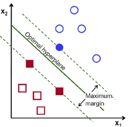
Basically, the idea in SVM is to fit a line (optimal hyperplane) between two differ-ent classes in a multi-dimensional dataset so that the distance between marginal levels is as great as possible and not a single data point exists between the marginals [2]. That has been done in Figure 2.1.
Figure 2.1: Classifying a 2-dimensional dataset with SVM. Source: <http://docs.opencv.org/2.4/doc/tuto-rials/ml/introduction_to_svm/introduction_to_svm.html>.
2.3.
Neural Networks
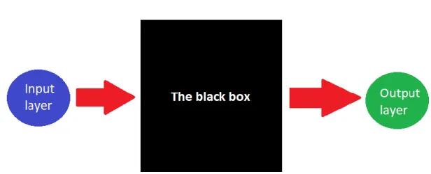
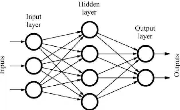
Neural networks are a small part of artificial intelligence (AI) [3]. A single neural network consists of layers of similar neurons. Usually it has at least an input layer and an output layer. There is a black box between the input and output layers as in Figure 2.2. The process that happens in the black box is supervised learning if we have specified the ideal output [3]. If ideal outputs are not provided, then the process is unsupervised learning [3]. In supervised learning we teach the neural network to give the ideal output, and in unsu-pervised learning we teach the network to group the input data [3].
Figure 2.2: A neural network with input layer, output layer and black box between them.
The input and output patterns are arrays that consist of floating-point numbers. For example, the input could be [1.00, 4.35, 0.38] and the output could be [2.84, −5.02]. Now we say that the input has three neurons and the output has two neurons. The number of neurons does not change, even if you restructure the interior of the neural network.
When a neural network is created, it has to be trained. Training is the process in which the neural network is adapted to make predictions from data [3].
2.3.1.
Artificial Neural Network (ANN)
An artificial neural network (ANN) is a type of neural network that consists of artificial neurons. The artificial neuron receives input from one or more sources. This input is often floating-point or binary.
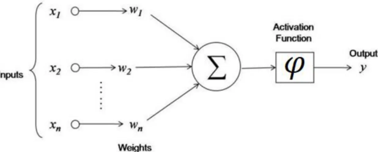
An artificial neuron multiplies the inputs by a weight. Then it adds these multipli-cations and passes this sum to a function 𝑓 that we define as
𝑓(𝑥𝑖, 𝑤𝑖) = 𝜑 (∑(𝑤𝑖∗ 𝑥𝑖) 𝑛
𝑖=1
)
where 𝑥𝑖 are the inputs, 𝑤𝑖 are the weights, 𝜑 is an activation function and 𝑛 is the number of the inputs. The activation function 𝜑 defines the output 𝑦 of the inputs as in Figure 2.3.
Figure 2.3: A detailed view of ANN. Source: <https://www.innoarchitech.com/artificial-intelligence-deep-learning-neural-networks-explained/>.
Figure 2.3 shows an artificial neural network in a very detailed form. Usually, when a neural network is presented as a diagram, the activation function and intermediate out-puts are not shown. That kind of diagram can be seen in Figure 2.4.
Figure 2.3 and Figure 2.4 show ANNs with only one building block. However, ANN can also consist of several artificial neurons that are chained together as in Figure 2.5.
Figure 2.5: ANN with multiple artificial neurons.
In general, the layers between input and output layers are called hidden layers [3]. The number of hidden layers determines the name of the network architecture. The neural network in Figure 2.5 presents an example of a two-hidden-layer network: neurons 𝑁1
and 𝑁2 form the first hidden layer, and 𝑁3 is the only neuron in the second hidden layer.
2.3.2.
Recurrent Neural Network (RNN)
Recurrent neural network (RNN) is a type of artificial neural network in which the con-nections do not have to flow only from one layer to the next [3]. In other words, connec-tions are not forced to go only from input layer to output layer. They can come back to
the neuron itself, go to a neuron on the same level or go to a neuron on a previous layer. That is called a recurrent connection [3]. An example of RNN is presented in Figure 2.6. The use of RNNs might be challenging because recurrent connections create infi-nite loops if the network does not know when to stop looping. There are three ways to prevent those endless loops: using context neurons, calculating output over a fixed num-ber of iterations, or calculating output until neuron output stabilizes [3, 4].
A simple RNN usually uses context neurons [3]. It is a special type of neuron that remembers its input and provides that input as its output the next time that the network in calculated [4]. For example, if we first give 0.5 as input, the output will be 0 that is always the first output of a context neuron. If we after that give for example 0.6 as input, the output will be 0.5. The input connections are never weighted in context neurons, but of course the output can be weighted like any other connection in a network [4].
Figure 2.6: A recurrent neural network. Source: <http://blog.josephwilk.net/ruby/recurrent-neural-net-works-in-ruby.html>.
2.3.2.1 Elman Neural Network
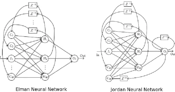
Elman neural network is a type of RNN from 1990, introduced by Elman [4]. This neural network provides pattern recognition to time series. There is one input neuron for each stream that you use to predict and one output neuron for each time slice that you try to predict. There is a single-hidden layer between input and output layers. A layer of context neurons takes its input from the hidden layer output and feeds back into the same hidden layer. Thus, the context layers have the same number of neurons as the hidden layer [4].
2.3.2.2 Jordan Neural Network
Jordan neural network is a type of RNN from 1993, introduced by Jordan [4]. Is has been created to control electronic systems. It has many similarities with Elman neural network but the difference between then is that in Jordan neural networks the context neurons can be fed from the output layer instead of the hidden layer. The output layers can also have recurrent connections to themselves with no other connections [4].
Figure 2.7: Examples of Elman and Jordan neural network. Source: <http://www.turingfinance.com/mis-conceptions-about-neural-networks/>.
Figure 2.7 presents examples of Elman and Jordan neural networks. In this figure we can also see 𝑧−1 nodes that complete 𝑧-transforms to neurons.
2.3.2.3 Long Short-Term Memory (LSTM)
Long short-term memory (LSTM) is a special type of RNN, introduced by Hochreiter and Schmidhuber in 1997 [5], and improved by Gers et al. in 2000 [6]. LSTM is an ANN that contains LSTM units instead of other network units [3]. For the LSTM units, it is typical that there are no activation functions within the recurrent components. It is typical that LSTM contains blocks that contain several LSTM units [3].
LSTM blocks contain three or four gates [3]. The gates are implemented with lo-gistic functions to compute a value between 0 and 1. The gates control the flow of infor-mation into or out of the memory of the LSTM blocks [3]. There is an input gate to control when new values are allowed to flow into the memory, a forget gate to control the process in which the values remain in the memory, and an output gate to control the process in which the values in memory are used to compute the output activation of the block [3].
A memory cell is a more complex LSTM unit. It is built around a central linear unit with a fixed self-connection. The memory cell gets input from the gate units and it can just flow the information through the block unchanged [3].
2.3.2.4 Gated Recurrent Unit (GRU)
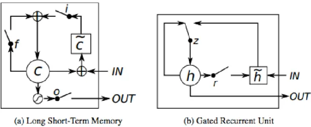
Gated recurrent unit (GRU) is a gating mechanism in RNN from 2014 [7]. It can be seen as a simplified version of LSTM. GRU does not have as many parameters as LSTM. For example, GRU does not have any output gate. The differences between LSTM and GRU can be seen in Figure 2.8.
Figure 2.8: LSTM and GRU. In (a), we can see input, forget and output gates 𝑖, 𝑓 and 𝑜, the memory cell
𝑐 and the new memory cell content 𝑐̃. In (b), we can see reset and update gates 𝑟 and 𝑧, the activation ℎ
and the candidate activation ℎ̃. Source: <https://deeplearning4j.org/lstm.html>.
2.3.3.
Feedforward Neural Network (FFNN)
Feedforward neural network (FFNN) is a very common type of an artificial neural net-work [3]. The term feedforward describes how FFNN processes and recalls patterns. Every layer contains connections to the next layer but there are no connections that move backward [3]. Thus, FFNN does not contain cycles and it is then different from RNN. An example of FFNN is presented in Figure 2.9.
Figure 2.9: A sample of FFNN. Source: <https://www.researchgate.net/figure/234055177_fig1_Figure-61-Sample-of-a-feed-forward-neural-network>.
2.3.4.
Self-Organizing Map (SOM)
A self-organizing map (SOM) is a type of neural network that applies unsupervised learn-ing. It has been published in 1988 by Kohonen [8]. SOM consists of input and output neurons and it is used to classify the input data into one of several groups. Training data is provided, as well as the number of the groups into which we wish to classify the data. SOM classifies together the values that have the most similar characteristics [3].
This process is very similar to clustering algorithms like 𝑘-means clustering. The difference is that SOM can continue classifying new data beyond the initial data set that was used for training. SOM is unsupervised, so it figures out the data groups itself, based on the training data, and then it classifies any future data into similar groups [3].
When the algorithm presents patterns to the input layer, the output neuron is the winner when it contains the weights most similar to the input [3]. This similarity is cal-culated by comparing the Euclidean distance between the set of weights from each output neuron. The shortest distance wins.
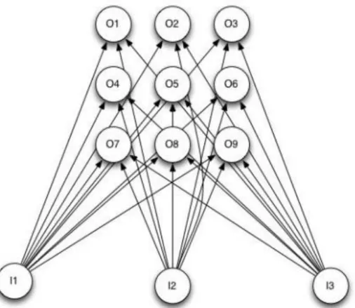
Figure 2.10: SOM with three input neurons and nine output neurons arranged in three-by-three grid. Source: [3].
2.4.
Deep Learning
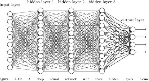
Deep learning is a relatively new set of training techniques for multilayered neural net-works [3]. It provides several algorithms that can train complex types of neural netnet-works. We can talk about deep learning when our neural network has more than two hidden layers [3] as an example network in Figure 2.11.
Figure 2.11: A deep neural network with three hidden layers. Source: <https://stats.stackexchange.com/questions/234891/difference-between-convolution-neural-network-and-deep-learning>.
2.4.1.
Deep Belief Neural Network (DBNN)
One of the first applications of deep learning was the deep belief neural network (DBNN) [3]. It is simply a regular belief network with many layers. Belief networks are different from regular FFNN because the input to DBNN must be binary, the output is the class to which the input belongs, and DBNN can generate plausible input based on a given out-come [3]. The input of FFNN is a decimal number, the output can be a class or a numeric prediction, and FFNNs cannot perform like the DBNNs [3].
2.4.2.
Convolutional Neural Network (CNN)
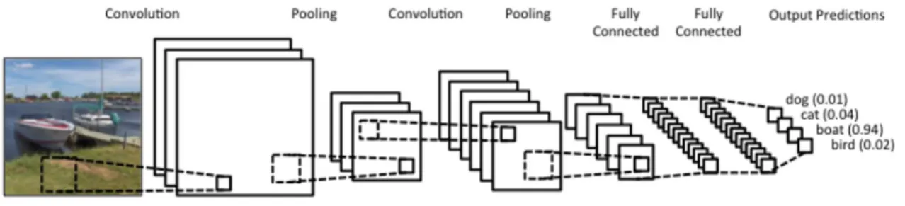
Convolutional neural network (CNN) is a special kind of neural network that processes data with a grid-like topology [3]. CNN has been originally created in 1980 by Fukushima [3]. It has been widely used in medical sciences because it successes very well in practical applications. An example of CNN can be seen in Figure 2.12.
CNN has similarities with SOM. First, CNNs and SOMs do not follow the standard treatment of input vectors as the other neural networks do. Second, they map their input into 2D grids or higher dimension objects such as 3D boxes. The difference between CNN and SOM is that CNN takes image recognition to higher level of capability.
Figure 2.12: A CNN recognizing boat from a picture. Source: <http://www.wildml.com/2015/11/under-standing-convolutional-neural-networks-for-nlp/>.
2.4.2.1 Convolutional layer
One typical layer of CNN is a convolutional layer that uses mathematical convolution to process the data [3]. Convolution is an operation on two functions 𝑓 and 𝑔 that generates a new function 𝑓 ∗ 𝑔. Convolution can be defined as
(𝑓 ∗ 𝑔)(𝑡) = ∫ 𝑓(𝑡 − 𝑥)𝑔(𝑥)𝑑𝑥 ∞
−∞
.
Convolution is commutative, and thus we can equally define it as
(𝑓 ∗ 𝑔)(𝑡) = ∫ 𝑓(𝑥)𝑔(𝑡 − 𝑥)𝑑𝑥 ∞
−∞
.
When the functions 𝑓 and 𝑔 are discrete, the convolution is defined as
(𝑓 ∗ 𝑔)(𝑛) = ∑ 𝑓(𝑘)𝑔(𝑛 − 𝑘) ∞
𝑘=−∞
.
Often, when the mathematical convolution is applied in machine learning, the input is a finite multidimensional data array and the kernel is a multidimensional array of variables that are adapted by the learning algorithm. The convolutions are usually used to over more than one axis at a time [3].
The main purpose for a convolutional layer is to detect features such as edges, lines, blobs of color and other visual elements [3]. To detect these features, the convolutional layer uses filters that are square-shaped objects that scan over the image. The more filters we give to a convolutional layer, the more features it can detect.
2.4.2.2 Max-pool layer
pool layers downsample a 3D box to a new one with smaller dimensions [3]. Max-pool layers are typically placed to follow a convolutional layer as in Figure 2.13. In this layer, the size of the dimensions of the 3D boxes are decreased.
Figure 2.13: An example of an operation in a max-pool layer. Source: <http://cs231n.github.io/convolu-tional-networks/>.
2.4.2.3 Dense layer
Dense layer is a layer type that is also used in FFNNs [3]. It connects every neuron in the previous layer’s output 3D box to each neuron in the dense layer. Then it passes the result vector through an activation function.
3.
SVM and Deep Learning in Medical Sciences
In this chapter we will study three different medical researches in which SVM and some deep learning methods are applied. The goal is to present the problems and what kind of methods have been used to solve them.
3.1.
SVM in classification of medical images
Vanitha and Venmathi (2011) [9] wanted to find a method to identify microbiological types without human supervision. In other words, they wanted to find a suitable learning method to classify bacterial types from medical images. Finally, they built a method that consists of three steps:
1. Pre-processing 2. Feature extraction
3. Bacteria classification using support vector machine (SVM) classifier. These steps are presented in Figure 3.1.
Figure 3.1: The process diagram. Source: [9].
In the first step, the goal is simply to remove the noise from the image that is given as input data. This is required, because the feature extraction in the next step gives poor results without this step.
The second step consists of three approaches: statistical approach, syntactic or structural approach and spectral approach. In the statistical approach, there is a multidi-mensional vector that presents a set of statistically extracted features that define the pat-tern. In the syntactic approach, texture primitives that define the texture are spatially or-ganized according to placement rules to generate complete pattern. In the syntactic pat-tern recognition, a formal analogy is drawn between the language syntax and the struc-tural pattern. In the spectral approach, the textures are defined by spatial frequencies and evaluated by the texture’s autocorrelation function.
The third step is about using SVM to complete the bacterial classification.
3.1.1.
Using SVM
Before presenting the use of SVM, the used variables are defined as follows: 1. Let 𝒙 be the input vector with dimension 𝑚0.
2. Let 𝑚1 be the dimension of the feature space.
3. Let 𝑤𝑗 be the linear weights that connect the feature space to the output space (for
𝑗 = 1 to 𝑚1).
4. Let 𝜑𝑗(𝒙) be nonlinear transformations from the input space to the feature space
(for 𝑗 = 1 to 𝑚1). These transformations represent the input supplied to the weights 𝑤𝑗 via the feature space.
5. Let 𝑏 be the bias, 𝛼𝑖 be the Lagrange coefficients and 𝑑𝑖 be the corresponding
target outputs (for 𝑖 = 1 to 𝑁).
The hyperplane acting as the decision surface is defined as
∑ 𝛼𝑖𝑑𝑖𝐾(𝒙, 𝒙𝑖) = 0 𝑁
𝑖=1
where 𝐾(𝒙, 𝒙𝑖) = 𝜑𝑇(𝒙)𝜑(𝒙𝑖) is the inner product of two vectors that are induced in the
feature space by 𝒙 and input pattern 𝒙𝑖 pertaining to the 𝑖𝑡ℎ example. This term is referred
to as inner-product kernel where 𝑤 = ∑𝑖=1𝑁 𝛼𝑖𝑑𝑖𝜑(𝒙𝑖), 𝜑(𝒙) = [𝜑0(𝒙), … , 𝜑𝑚1(𝒙)] 𝑇
,
𝜑0(𝒙) = 1 and 𝑤0 = 𝑏.
3.1.2.
Results
The input data consisted of 180 bacterial images. 120 images were used for training and remaining 60 images were used for testing. The pattern vectors (features) were extracted from those images and provided to SVM as input. The classification accuracy and error rate were defined as
𝐴𝑐𝑐𝑢𝑟𝑎𝑐𝑦 = 𝑁𝑢𝑚𝑏𝑒𝑟 𝑜𝑓 𝑐𝑜𝑟𝑟𝑒𝑐𝑡𝑙𝑦 𝑐𝑙𝑎𝑠𝑠𝑖𝑓𝑖𝑒𝑑 𝑏𝑎𝑐𝑡𝑒𝑟𝑖𝑎𝑙 𝑖𝑚𝑎𝑔𝑒𝑠 𝑇𝑜𝑡𝑎𝑙 𝑛𝑢𝑚𝑏𝑒𝑟 𝑜𝑓 𝑏𝑎𝑐𝑡𝑒𝑟𝑖𝑎𝑙 𝑖𝑚𝑎𝑔𝑒𝑠
and
𝐸𝑟𝑟𝑜𝑟 𝑅𝑎𝑡𝑒 =𝑁𝑢𝑚𝑏𝑒𝑟 𝑜𝑓 𝑚𝑖𝑠𝑐𝑙𝑎𝑠𝑠𝑖𝑓𝑖𝑒𝑑 𝑏𝑎𝑐𝑡𝑒𝑟𝑖𝑎𝑙 𝑖𝑚𝑎𝑔𝑒𝑠 𝑇𝑜𝑡𝑎𝑙 𝑛𝑢𝑚𝑏𝑒𝑟 𝑜𝑓 𝑏𝑎𝑐𝑡𝑒𝑟𝑖𝑎𝑙 𝑖𝑚𝑎𝑔𝑒𝑠 .
The process was completed 6 times. Each time the training set contained 20 images and the test set contained 10 images.
The SVM finally gave a classification efficiency of 97.5% during training phase and 93.33% during testing phase. The results were pretty good, and the classification accu-racy can still be improved by extracting more features and providing a bigger training data set.
3.2.
Multi-dimensional RNNs in segmentation of 3D data
Andermatt et al. (2016) [10] present a supervised deep learning method that is used to automatically segment 3D volumes of biomedical image data. The method is based on a neural network that consists of multi-dimensional gated recurrent units. This method gives accurate results without a huge amount of training data and without advanced data pre- or postprocessing.
Automatic segmentation of biomedical volumetric data is a challenging problem because of high dimensionality, imaging noise, artifacts and other factors. This problem could be solved with feed-forward neural networks, but we would then need a large num-ber of layers. For that reason, the authors have used deep RNNs as their method.
The dataset was the publicity available MrBrainS challenge dataset that consists of 5 labeled samples and 15 testing samples. The training data contained a label map for training and another label map for testing. The training map consists of classes for cortical gray matter (GM), basal ganglia, white matter (WM), WM lesions, cerebrospinal fluid (CSF), ventricles, cerebellum, brainstem and background. The testing map only defines classes for GM, WM and CSF.
Andermatt et al. applied two types of RNNs in their research: long short-term memory (LSTM) and gated recurrent unit (GRU). We will now check the details of how these RNNs have been applied.
3.2.1.
Using RNNs
3.2.1.1 LSTM
The authors used the multi-dimensional Long Short-Term Memory (MD-LSTM) called PyraMiD-LSTM. It defines two LSTMs for each spatial dimension: the first one pro-cesses data along that dimension, and the second one in the opposite direction.
3.2.1.2 GRU
The standard GRU is defined as
𝑟𝑗 = 𝜎([𝑊𝑟𝒙]𝑗+ [𝑈𝑟ℎ𝑡−1]𝑗), 𝑧𝑗 = 𝜎([𝑊𝑧𝒙]𝑗+ [𝑈𝑧ℎ𝑡−1]𝑗), ℎ̅𝑡𝑗 = 𝜑([𝑊𝒙]𝑗+ [𝑈(𝑟 ⊙ ℎ 𝑡−1)]𝑗), ℎ𝑡𝑗 = 𝑧𝑗⊙ ℎ 𝑡−1 𝑗 + (1 − 𝑧𝑗) ⊙ ℎ̅ 𝑡 𝑗 ,
where 𝒙 is the input data, 𝑟𝑗 is the reset gate, 𝑧𝑗 is the update gate of the hidden unit 𝑗
and the activation is performed in ℎ𝑗. The operator ⊙ represents an elementwise
multi-plication. The functions 𝜎(∙) and 𝜑(∙) stand for the logistic function and the hyperbolic tangent. 𝑊 and 𝑈 are the weight matrices for the current input and last step’s output data respectively. Now when the goal is to process 3D data, these equations have been trans-formed in forms 𝑟𝑗 = 𝜎 (∑(𝑥𝑖 ∗ 𝑤 𝑟 𝑖,𝑗 ) 𝐼 𝑖 + ∑(ℎ𝑡−1𝑘 ∗ 𝑢 𝑟 𝑘,𝑗 ) 𝐽 𝑘 + 𝑏𝑟𝑗), 𝑧𝑗 = 𝜎 (∑(𝑥𝑖 ∗ 𝑤𝑧𝑖,𝑗) 𝐼 𝑖 + ∑(ℎ𝑡−1𝑘 ∗ 𝑢𝑧𝑘,𝑗) 𝐽 𝑘 + 𝑏𝑧𝑗),
ℎ̅𝑡𝑗 = 𝜑 (∑(𝑥𝑖∗ 𝑤𝑖,𝑗) 𝐼 𝑖 + 𝑟𝑗⊙ ∑(ℎ 𝑡−1𝑘 ∗ 𝑢𝑘,𝑗) 𝐽 𝑘 + 𝑏𝑗), ℎ𝑡𝑗 = 𝑧𝑗⊙ ℎ𝑡−1𝑗 + (1 − 𝑧𝑗) ⊙ ℎ̅𝑡𝑗,
where ∗ represents a convolution and 𝑏 is a bias. Because these equations apply convo-lution, this is called convolutional GRU (C-GRU). Its architecture is presented in Figure 3.2.
Figure 3.2: The architecture of C-GRU. Source: [10].
The multi-dimensional GRU (MD-GRU) consists of two times 𝐷 C-GRUs, where
𝐷 is the dimensionality of the image data. One C-GRU is needed for each of the two directions. The architecture of MD-GRU is presented in Figure 3.3.
Figure 3.3: The architecture of MD-GRU. Source: [10].
The architecture of the whole network can be seen in Figure 3.4.
Figure 3.4: The network architecture. Source: [10].
3.2.2.
Results
The preprocessing step started by using a Gaussian smoothed image that was then sub-tracted from the original images to produce highpass filtered volumes. In three training steps, the subvolume size was first increased from 64 × 64 × 8 voxels to 128 × 128 ×
12 and then to 200 × 200 × 15. In the testing phase, the volume was divided into a grid of equally sized subvolumes of 120 × 120 × 8.
The authors wanted to compare MD-GRU and MD-LSTM by running the same setup with the multi-dimensional RNN layers first on MD-GRU and then on MD-LSTM. The results can be found in the Table 1.
Table 3.1: The accuracy values in percent for gray and white matter (GM/WM), cerebrospinal fluid (CSF) and intracranial volume (ICV). Source: [10].
GM WM CSF ICV
MD-LSTM 88.09 90.08 82.62 97.56
MD-GRU 87.88 90.15 83.19 97.73
In the feasibility study, MD-GRU achieved comparable results to the MD-LSTM in less time with the same settings. This means that MD-GRU has a great potential for the segmentation of volumetric images.
3.3.
CNN in chest pathology
Bar et al. (2015) [11] have presented a CNN that is applied in pathology detection for chest radiograph data.
3.3.1.
Using CNN
The authors used the DeCAF (“Deep Convolutional Activation Feature”) [12] implemen-tation of CNN that can be seen in Figure 3.5. DeCAF was originally presented by Do-nahue et al. (2013). It has been used in generic visual recognition and it is a good choice when the goal is to recognize some patterns from images.
The main interests of the CNN were 5th layer (Decaf5), 6th layer (Decaf6) and 7th
layer (Decaf7). Decaf5 contains 9216 activations of the last convolutional layer and is the
first set of activations that has been fully propagated through the convolutional layers of the network. Decaf6 contains 4096 activations of the first fully-connected layer. Decaf7
Figure 3.5: CNN schematic view of the DeCAF CNN. Source: [11].
The CNN was trained with ImageNet that is a well-known non-medical image da-tabase. In the training step, the CNN was trained over a subset of more than one million images that are categorized into 1000 categories.
The second baseline descriptor was the “Picture Codes” (PiCoDes) descriptor. It is a compact high-level representation of popular low-level features (SIFT, GIST, PHOG and SSIM [13]) which is optimized over a subset of the ImageNet dataset containing approximately 70,000 images. PiCoDes makes it possible to binarize images with high performance rates on object category recognition. Local Binary Patterns (LBP) [14] and GIST were used as descriptors.
The classification was done using SVM with linear kernel using leave-one-out-cross-validation. There were three accuracy measurements: Sensitivity, Specificity and the area under the ROC curve (AUC). Sensitivity and Specificity are derived based on the optimal cut point on the ROC. All the values were standardized (except the binary ones), so that each column has its mean subtracted and is divided by its standard devia-tion.
Figure 3.6: Algorithm flowchart. Source: [11].
3.3.2.
Results
The dataset cosists of 93 frontal chest x-ray images from Sheba Medical Center. 37 im-ages showed a healthy chest, 24 imim-ages showed an enlarged heart and 14 imim-ages showed a right pleural effusion. The results can be seen in the Table 3.2, Table 3.3 and Table 3.4.
Table 3.2: The accuracy levels in Right Pleural Effusion Condition process in percent. Source: [11].
Low Level High Level Deep Fusion
LBP GIST PiCoDes Decaf L5 Decaf L6 Decaf L7 PiCoDes+Decaf L5
Sensitivity 71.00 79.00 79.00 93.00 86.00 86.00 93.00
Specificity 77.00 92.00 91.00 84.00 86.00 80.00 84.00
Table 3.3: The accuracy levels in Healthy vs. Pathology process in percent. Source: [11].
Low Level High Level Deep Fusion
LBP GIST PiCoDes Decaf L5 Decaf L6 Decaf L7 PiCoDes+Decaf L5
Sensitivity 65.00 68.00 59.00 73.00 89.00 76.00 81.00
Specificity 61.00 66.00 79.00 80.00 64.00 64.00 79.00
AUC 63.00 72.00 72.00 78.00 79.00 72.00 79.00
Table 3.4: The accuracy levels Enlarged Heart Condition process in percent. Source: [11].
Low Level High Level Deep Fusion
LBP GIST PiCoDes Decaf L5 Decaf L6 Decaf L7 PiCoDes+Decaf L5
Sensitivity 75.00 79.00 79.00 88.00 79.00 79.00 83.00
Specificity 78.00 81.00 84.00 78.00 88.00 77.00 84.00
4.
Deep Learning in Non-Medical Applications
Deep learning is widely used also in non-medical applications. In this chapter we study briefly some other common applications of deep learning methods.
4.1.
Natural Language Processing (NLP)
Natural language processing (NLP) is a field of computer science that focuses on inter-actions between computers and human (natural) languages [15]. Artificial intelligence (AI) is widely used to make computers to understand both written and spoken language and to create that kind of language by themselves [15].
NLP is a very common application of deep learning [16]. The problems in NLP are too complex to solve with traditional methods but not too complex to solve with deep neural networks.
A common deep learning method in NLP is a RNN. It is widely used especially in speech recognition [17]. The strength of RNN in speech recognition is that we can teach RNN to process all the previous letters and the previous words, not just the current one. Thus, RNN uses all the useful information in this process and gives more accurate re-sults than the other methods that can only process the current word without the previous knowledge.
RNN is also used in text classification [18]. The power of RNN in text classifica-tion is that also in this case RNN processes the text as a sequence and uses all the previ-ous words when classifying a single word. Figure 4.1 shows an example of RNN that classifies the words of a text “The first fifteen minutes were dry, but by the end I really enjoyed the lecture.” into positive, neutral and negative classes.
Figure 4.1: A recurrent neural network classifying the words a text into positive (+), neutral (0) and neg-ative (-) classes. Source: <http://cs224d.stanford.edu/>.
Also CNNs have been used in text classification [19]. The sentences are usually given as input vectors to CNN. Then the CNN processes those input vectors in a very similar way as pixels of an image. An example of that process can be seen in Figure 4.2.
Figure 4.2: A text classification example with CNN. Source: <http://www.wildml.com/2015/12/imple-menting-a-cnn-for-text-classification-in-tensorflow/>.
4.2.
Robotics
Robotics is a field of engineering and science that is about design, construction, opera-tion and use of robots [20]. The robots apply AI and thus deep learning is used when the robots have to do something “intelligent” that is hard to implement with more tradi-tional methods [21].
A well-known example of intelligent robots are digital cameras that recognize faces of people before taking the picture. More complex examples are robots that recog-nize different shapes or different colors.
To recognize more and more complex patterns, the robots use deep and complex neural networks [21]. Deep learning algorithms have been used, for example, in phones that recognize the fingerprint of the user.
5.
Tools for Deep Learning
In this chapter we focus on tools for deep learning. We present R and Python program-ming languages, some of their libraries and other tools that are usable with them. The principal references of this chapter are the documentations of the presented tools.
Visualization is an important part of machine learning [22], and so it is important in deep learning [23]. For that reason, we are not only interested in the methods for ana-lyzing the data but we also wish to find tools to visualize the processes.
5.1.
R language
R is a language and environment for statistical computing and graphics. It is based on S language and can be seen as a different implementation of S [24].
R provides a large scale of statistical and graphical techniques. For example, it can be used for linear and nonlinear modelling, classical statistical tests, time-series analysis, classification and clustering [24].
There are several R libraries that provide methods for machine learning and deep learning. Now we will list at some of them and study their properties briefly.
nnet is a simple and widely used R library to build neural networks. However, it does not provide tools for complex neural networks because it lets the user to create only one hidden layer. But for a simple neural computing this is a good choice. nnet can also be used to plot the neural networks. Figure 5.1 shows an example of a one-hidden-layer network that has been created and visualized with nnet.
Figure 5.1: A one-hidden-layer neural network created and visualized with nnet. In the picture, I1, …, I8 are the input nodes, H1, …, H10 are the hidden neurons, O1 is the output node, and B1 and B2 are bias nodes. Source: <https://beckmw.wordpress.com/tag/neural-network/>.
MXNetR is a library that works under MXNet [25]. This library provides tools for complex FFNNs and for CNNs too. MXNetR also provides a simple method to visualize the deep neural networks that we have created with it. Figure 5.2 shows an example of a deep neural network that has been visualized with MXNetR. The CNNs in MXNet are LeNet [26] networks. The strengths of MXNetR are that it is very fast and easy to use.
Figure 5.2: A deep neural network visualized with MXNetR. Source: <https://www.r-bloggers.com/deep-learning-in-r-2/>.
darch is a library for deep belief neural networks (DBNN) and Boltzmann ma-chines. It is also very easy to use. For example, it requires only one function to train the network.
deepnet is a small library that does not provide many functions but is still very powerful. With deepnet library we can create deep FFNNs, DBNNs or restricted Bolzmann machines and train them with only function.
H2O is a library that is based on H2O open-source software platform [27]. H2O has a very special syntax and it is different from many other R libraries, but still it is easy
to use. H2O provides a very large scale of tools for deep learning and, as MXNet, it is very fast. H2O also supports distributed computations and provides a web interface.
deepr is a library that was developed when H2O library was not yet available. deepr does not implement any deep learning algorithms but it forwards its tasks to H2O.
dplyr is a library that provides powerful methods to transform and summarize tab-ular data with rows and columns in R. With dplyr, we can manipulate data in several ways with a very short code. This makes the data preprocessing much easier.
mice is another R library to help with the data preprocessing. This library has been designed to find missing values from the data and to handle them in an appropriate way. mice provides several functions for the missing value handling process.
ggplot2 is a graphical library that provides very powerful visualizations for the results. Figure 5.3 shows an example visualization of the results of some clustering algo-rithm.
Figure 5.3: The results of some clustering algorithm visualized with ggplot2. Source: <http://www.sthda.com/english/wiki/ggfortify-extension-to-ggplot2-to-handle-some-popular-packages-r-software-and-data-visualization>.
Kohonen is a library to build SOMs for the data. The library name comes from Finnish academic and researcher Teuvo Kohonen who is known as the creator of SOMs. This library contains simple functions to process the data and also methods to visualize the results as in Figure 5.4.
Figure 5.4: A visualization of the results of a SOM. The nodes that have the same color belong to the same cluster and are more similar than two nodes from different clusters. The nodes are some cases from the data. Source: <http://www.shanelynn.ie/self-organising-maps-for-customer-segmentation-using-r/>.
5.2.
Python language
Python [28] is a programming language that provides many useful libraries for deep learning. Now we will list some of them as examples.
NumPy (“Numeric Python” or “Numerical Python”) is an open library for scientific computing with Python. It provides useful mathematical tools, such as multi-dimensional arrays, matrices and a large scale of mathematical functions.
SciPy (“Scientific Python”) is an open source library for scientific computing and technical computing. It builds on the NumPy array object and is actually a part of the NumPy stack.
Scikit-learn is machine learning library that interoperates NumPy and SciPy. It pro-vides several machine learning algorithms for classification, regression and clustering, like support vector machine, random forests and 𝑘-means clustering.
Pandas is a library for data manipulation and analysis. It provides data structures and operations to process numerical tables and time series.
Matplotlib is a library for Python that provides methods for data visualization. Fig-ure 5.5 presents a simple neural network that has been visualized with Matplotlib.
Figure 5.5: A simple neural network visualised with Matplotlib. Source: <https://github.com/mi-loharper/visualise-neural-network>.
Seaborn is a visualization library that has been built on Matplotlib. It provides tools for advanced visualization. In other words, it can be used to visualize complex result of some analysis, as in Figure 5.6.
Figure 5.6: Advanced visualization with Seaborn. Source: <http://seaborn.pydata.org/generated/sea-born.pairplot.html>.
Theano [29] is a numerical computation library for machine learning. Its computa-tions are expressed using NumPy. Theano provides tools, for example, for convolution, pooling and long-term serialization, and it can be used to implement complex neural net-works.
Pylearn2 is a machine learning library that is mostly built on Theano. It is very good choice for neural computing as Theano, but the speciality in Pylearn2 is that it has been planned to be so flexible that the user can do anything with it.
Caffe is a deep learning framework that supports many types of deep learning archi-tectures, like CNNs and LSTMs. It is suitable for image classification and segmentation. There is also Caffe2 that is built on Caffe but includes new features.
PyNeurGen is a very large library that supports deep and complex neural networks. The user can create multiple hidden layers and use different types of neurons.
5.3.
Spark
Apache Spark is a fast and general cluster-computing engine for large-scale data pro-cessing. It can be used with R and Python, but also with Java and Scala. As R and Python, Spark also has its own libraries for machine learning and deep learning.
MLLib (“Machine Learning Library”) is a machine learning library for Spark. This library offers very large scale of machine learning operations and it is easy to use. There are, for example, basic statistical operations like correlation and hypothesis testing, but also functions for support vector machine and 𝑘-means clustering.
SparkNet is a library for training deep neural networks in Spark. It provides tools, for example, for convolutional layers and max-pool layers so that the user can implement a CNN.
Spark can be used in R with a library SparkR or with sparklyr. In Python it can be used with library pyspark.
5.4.
TensorFlow
TensorFlow is an open source software library that was developed by Google Brain Team [30]. It was released in 2015. TensorFlow can be used with Python and it provides a large scale of machine learning methods, especially powerful methods to build deep and com-plex neural networks.
5.4.1.
Implementing RNN
Now we will look at how we could implement an RNN in TensorFlow. First of all, Ten-sorFlow provides a module tf.contrib that includes many RNN operations. It contains the base interface for all RNN cells, tf.contrib.rnn.RNNCell. We can also find specific inter-faces for special kinds of RNN cells. For example, with tf.contrib.rnn.LSTMCell we can implement an LSTM cell, and with tf.contrib.rnn.GRUCell we can implement a GRU cell. With tf.contrib.rnn.MultiRNNCell we can implement an RNN cell that is composed sequentially of multiple simple cells.
The easiest way to implement the whole RNN with TensorFlow is to use class
tf.contrib.rnn.static_rnn. It asks a cell and the inputs as parameters and then creates a RNN that computes the outputs. For more complex RNNs, we have classes like tf.con-trib.rnn.stack_bidirectional_dynamic_rnn and tf.contrib.rnn.static_state_saving_rnn.
6.
Conclusion
Deep learning is a field of machine learning that usually provides amazingly accurate results. Basically, deep learning is about solving tricky problems with deep and complex neural networks.
The deep learning methods are capable to solve problems that would be extremely hard or even impossible to solve with traditional machine learning or statistical methods. This has been noticed in many fields of science and nowadays deep learning methods are used to solve practical problems that have not had any clear solutions before.
In medical applications, the common problem is that we have to recognize some patterns from images. A support vector machine is good choice when the pattern is not too complex. When it is complex, machine learning methods do not help us. Thus, we need deep learning methods to find the patterns from the images. Multi-dimensional re-current neural networks and convolutional neural networks are deep and complex neural networks that process images very carefully by taking the images through several layers. The accuracy of the result grows when we add new layers into the networks.
The results of deep learning methods in medical applications are not yet shown in our everyday life but there are other deep learning applications that are. We have learned that deep learning methods are applied in natural language processing and in robotics. If we think about writing with computer or phone, we can notice that sometimes there is an algorithm that tries to automatically recognize our mistakes and to fix them. We can also find some voice control facilities from the modern smartphones. These are examples of natural language processing applications in our everyday lives. Robotics are also close to us if we, for example, take pictures with a digital camera that recognizes faces of people, or use fingerprint locks in our phones.
There are several tools to implement the machine learning and deep learning meth-ods. R and Python are good choices for programming languages, and with them we can use several different libraries or specific tools like Spark or TensorFlow. When we com-bine these tools in our code, we can make very powerful codes that preprocess our data carefully, builds an appropriate neural network, trains it carefully, processes the data and visualizes the results.
Because deep learning is a relatively new field of science, most of the tools are also new. Actually new tools for deep learning are developed all the time. New methods are
needed, and of course people want to use tools that are easy to use but at the same time fast and capable to solve complex problems.
It seems that deep learning is currently doing some revolution in many sciences. Deep learning will surely be an important thing also in the future. It will give more and more power in data analysis and help us to develop new products, like voice command devices. In medical sciences, it can also provide so accurate results that doctors and biol-ogists find new treatment methods against some diseases. Thus, deep learning has a huge potential to change the world in some significant way.
Bibliography
[1] Marsland, S. (2015). Machine Learning: An Algorithmic Perspective, second edi-tion. CRC Press.
[2] Cortes, C., Vapnik, V. (1995). Support-Vector Networks. Machine Learning 20, 273-297.
[3] Heaton, J. (2015). Artificial Intelligence for Humans, Volume 3: Deep Learning and Neural Networks. Heaton Research Inc, USA.
[4] Lipton, Z., Berkowitz, J., Elkan, C. (2015). A Critical Review of Recurrent Neural Networks for Sequence Learning. <https://arxiv.org/abs/1506.00019v4>.
[5] Hochreiter, S., Schmidhuber, J. (1997). Long Short-Term Memory. Neural Compu-tation 9(8), 1735-1780.
[6] Gers, F. (2001). Long Short-Term Memory in Recurrent Neural Networks. PhD Thesis, Ecole Polytechnique Fédérale de Lausanne.
[7] Chung, J., Gulcehre, C., Cho, K., Bengio, Y. (2014). Empirical Evaluation of Gated
Recurrent Neural Networks on Sequence Modeling.
<https://arxiv.org/abs/1412.3555>.
[8] Kohonen, T. (1988). Self-Organization and Associative Memory, second edition. Springer Series in Information Sciences.
[9] Vanitha, L., Venmathi, A. (2011). Classification of Medical Images Using Support Vector Machine. International Conference on Information and Network Technol-ogy. IPCSIT vol. 4. IACSIT Press, Singapore.
[10] Andermatt, S., Pezold, S., Cattin, P. (2016). Multi-dimensional Gated Recurrent Units for the Segmentation of Biomedical 3D-Data. In: Medical Imaging. Vol. 9785 of Proceedings of the SPIE. p. 978510.
[11] Bar, Y., Diamant, I., Wolf, L., Greenspan, H. (2015). Deep Learning with non-medical training used for chest pathology identification. Medical Imaging. Vol. 9414 of Proceedings of the SPIE.
[12] Donahue, J., Jia, Y., Vinyals, O., Hoffman, J., Zhang, N., Tzeng, E., Darrell, T. (2013). DeCAF: A Deep Convolutional Activation Feature for Generic Visual Recognition. <https://arxiv.org/abs/1310.1531>.
[13] Oliva, A., Torralba, A. (2001). Modeling the Shape of the Scene: A Holistic Repre-sentation of the Spatial Envelope. International Journal of Computer Vision 42(3), 145-175.
[14] Ojala, T., Pietikäinen, M., Mäenpää, T. (2002). Multiresolution gray-scale and ro-tation invariant texture classification with local binary patterns. IEEE Trans. Pat-tern Analysis and Machine Intelligence, vol. 24, no. 7, pp. 971-987.
[15] Kibble, R. (2013). Introduction to Natural Language Processing. University of London, Department of Computing.
[16] Lopez, M., Kalita, J. (2017). Deep Learning applied to NLP. <https://arxiv.org/pdf/1703.03091.pdf>.
[17] G. Saon, H. Soltau, A. Emami, and M. Picheny. (2014). Unfolded Recurrent Neural Networks for Speech Recognition. Fifteenth Annual Conference of the International Speech Communication Association.
[18] Xu, J., Chen, D., Qiu, X., Huang, X. (2016). Cached Long Short-Term Memory
Neural Networks for Document-Level Sentiment Classification.
<https://arxiv.org/pdf/1610.04989.pdf>.
[19] Johnson, R., Zhang, T. (2015). Effective Use of Word Order for Text Categorization with Convolutional Neural Networks. Human Language Technologies: The 2015 Annual Conference of the North American Chapter of the ACL, pages 103–112. [20] Craig, J. (2005). Introduction to Robotics: Mechanics and Control, Third Edition.
Pearson Education, Inc.
[21] Lenz, I., Lee, H., Saxena, A. (2015). Deep Learning for Detecting Robotic Grasps. The Internal Journal of Robotics Research, 34(4-5):705-724.
[22] Keim, D., Rossi, F., Seidl, T., Verleyzen, M., Wrobel, S. (2012). Information Vis-ualization, Visual Data Mining and Machine Learning. Dagstuhl Reports, 2(2), pp. 58-83.
[23] Yosinski, J., Clune, J., Nguyen, A., Fuchs, T., Lipson, H. (2015). Understanding Neural Networks through Deep Visualization. <https://arxiv.org/abs/1506.06579>. [24] Paradis, E. (2002). R for Beginners. Montpellier (F): University of Montpellier.
[25] Tianqi, C., Mu, L., Yutian, L., Min, L., Naiyan, W., Minjie, W., Tianjun, X., Bing, X., Chiyuan, Z., Zheng, Z. (2015). MXNet: A Flexible and Efficient Machine
Learn-ing Library for Heterogenous Distributed Systems.
<https://arxiv.org/abs/1512.01274>.
[26] LeCun, Y., Bottou, L., Bengio, Y., Haffner, P. (1998). Gradient-Based Learning Applied to Document Recognition. Proc. IEEE, vol. 86, no. 11, pp. 2278-2324. [27] Candel, A., Parmar, V., LeDell, E., Arora, A. (2015). Deep Learning with H2O.
H2O.ai Inc.
[28] Haltermann, R. (2011). Learning to Program with Python. <https://www.cs.uky.edu/~keen/115/Haltermanpythonbook.pdf>.
[29] Bastien, F., Lamblin, P., Pascanu, R., Bergstra, J., Goodfellow, I., Bergeron, A., Bouchard, N., Bengio, Y. (2012). Theano: New Features and Speed Improvements. Deep Learning and Unsupervised Feature Learning NIPS 2012 Workshop.
[30] Goldsborough, P. (2016). A Tour of TensorFlow. <https://arxiv.org/pdf/1610.01178.pdf>.