MASTER’S THESIS
Lauri Nevasalmi
Forecasting multinomial stock returns using machine
learning methods
Tampere University
Faculty of Information Technology and Communication Sciences May 2019
Tampere University
Faculty of Information Technology and Communication Sciences
NEVASALMI, LAURI: Forecasting multinomial stock returns using machine learning methods
Master’s thesis, 43 p., 2 app. p. Computational Big Data Analytics May 2019
Abstract
In this thesis, the daily returns of the S&P 500 stock market index are predicted us-ing a variety of di¤erent machine learnus-ing methods. We propose a new multinomial classi…cation approach to forecasting stock returns. The multinomial approach can isolate the noisy ‡uctuation around zero and allows us to focus on predicting the more informative large absolute returns. Our in-sample and out-of-sample forecast-ing results indicate signi…cant return predictability from a statistical point of view. Moreover, all the machine learning methods considered outperform the benchmark buy-and-hold strategy in a real-life trading simulation. The gradient boosting ma-chine is the top-performer in terms of both the statistical and economic evaluation criteria.
Contents
1 Introduction 3
2 Methodology 6
2.1 Multinomial stock returns . . . 6
2.2 Machine learning methods . . . 8
2.2.1 k-Nearest neighbor classi…er . . . 8
2.2.2 Gradient boosting . . . 9
2.2.3 Random forest . . . 13
2.2.4 Neural networks . . . 15
2.2.5 Support vector machines . . . 17
2.3 Previous literature . . . 20
3 Data and model setup 24 3.1 Data . . . 24
3.2 Tuning parameter optimization . . . 27
4 Empirical results 30 4.1 Estimation results . . . 30
4.2 Economic in‡uence . . . 32
5 Conclusions 38
Bibliography 40
1
Introduction
Forecasting stock returns has attracted a tremendous amount of interest ever since the introduction of computers to economic forecasting. Kendall (1953) was among the …rst to reach the conclusion of no predictability in stock prices. Later Fama (1970) stated in the famous e¢cient market hypothesis that abnormal returns should not be possible to make by using historical data. But has the ever-growing amount of infor-mation and computational power in recent decades changed this relationship? State of the art machine learning methods, which can handle large amounts of informa-tion and discover complex relainforma-tionships in data, provide further insight if pro…table trading strategies can be discovered using past information.
The predictability of stock returns is a controversial subject. In a comprehensive study Welch and Goyal (2008) argue that the predictability found for the level of stock returns in the previous literature is time inconsistent and does not hold when new data is introduced. More recent work by Neely, Rapach, Tu and Zhou (2014), among others, challenge the view of Welch and Goyal (2008) by reporting statistically signi…cant predictability using more sophisticated forecasting methods.
Instead of the actual level of return another strand of literature focuses on predict-ing the binary sign of stock returns (i.e. directional predictability of stock returns). Leung, Daouk and Chen (2000) provide empirical results in favor of using the binary response variable instead of the actual level. Other studies reporting statistically sig-ni…cant predictability using monthly stock returns are for example Nyberg (2011) and Nyberg & Pönkä (2016). Christo¤ersen and Diebold (2006) show theoretically that sign predictability may exist even without the assumption of mean-predictability. Al-though the majority of the previous literature concerns predicting monthly returns, some more recent studies have reported predictability using daily returns as well (see e.g., Skabar, 2013; Fiévet & Sornette, 2018). The main objective in this thesis is to predict daily stock returns of the U.S. stock market (more speci…cally S&P 500 index returns) using di¤erent machine learning methods.
Directional prediction of stock returns is based on forecasting whether returns are greater than some pre-speci…ed threshold. Previous research mainly focuses on sign prediction, where this treshold is equal to zero, but some other alternatives have also been considered. Linton and Whang (2007) use the estimated unconditional quantiles of the return as a threshold. Chung and Hong (2007) express the thresh-old as multiples of the estimated standard deviation when forecasting the direction of exchange rates. Both studies …nd evidence of directional predictability in asset returns using di¤erent statistical testing procedures.
Directional prediction of stock returns has a close connection to the market tim-ing models considered by Merton (1981) and Pesaran & Timmermann (1995). Di-rectional prediction of stock returns leads to simple binary trading strategies which can be used to assess the economic signi…cance of the forecasting ability. Predicting the sign of stock returns involves a large amount of asset allocation decisions and the costs related to these transactions can be problematic when compared to the benchmark buy-and-hold strategy. This problem is even more alleviated with daily data (Becker & Leschinski, 2018).
By considering two di¤erent thresholds instead of just one the directional predic-tion problem becomes multinomial. The signal-to-noise ratio in stock returns is fairly low, especially with daily data (Becker & Leschinski, 2018). Chung and Hong (2007) argue that the informational content of large absolute returns may be more valuable whereas small returns are merely noise. It is also noted that the co-movement of individual stocks with the market portfolio is stronger with large absolute returns (see e.g., Longin & Solnik, 2001; Ang & Chen, 2002; Hong, Tu & Zhou, 2007). The multinomial response allows us to isolate some of the noise and put more emphasis on predicting the large absolute returns. The multinomial directional prediction also enables a richer set of possible trading strategies. For example one could choose between buying, holding and selling stocks instead of the binary buy or sell decision. To the best of our knowledge multinomial stock returns have not been utilized in previous economic research.
Our results con…rm the previous …ndings of sign predictability in stock returns. All the machine learning methods considered in this thesis produce multinomial classi…cation signi…cant from both the statistical and economical point of view. Each method is able to outperform the benchmark buy-and-hold strategy in a real-life trading simulation when trading costs are taken into account. Among the machine learning methods considered an ensemble method called gradient boosting is the top-performer in terms of both the classi…cation accuracy and the pro…ts from a real-life trading simulation.
The results also show how the predictability of large absolute returns tend to cluster around certain periods of time. This is in line with the …ndings of Krauss, Do & Huck (2017) and Fiévet & Sornette (2018) who notice increased predictability during high market turmoil. A closely related observation often reported in the …nancial literature is the higher return predictability during recession periods (see e.g., Henkel, Martin & Nardari, 2011; Cujean & Hasler, 2017). Events such as the …nancial crisis or the European debt crisis involve high volatility in the stock markets
but also highly pro…table trading opporturnities. Our results show that volatility in the stock market as measured by the VIX-index is the single most in‡uential predictor of next days’ stock returns.
The remainder of this thesis is organized as follows. The prediction problem and the di¤erent machine learning methods are presented in section 2. The dataset and the model selection process for di¤erent machine learning methods are described in section 3. The empirical analysis and the results are covered in section 4. Section 5 concludes.
2
Methodology
2.1
Multinomial stock returns
Financial literature usually focuses on the reward of holding a risky asset such as stocks compared to the risk-free investment. This excess return is denoted as
Zt =rt rft; (1)
where rt is the logarithmic daily return of the S&P 500 stock market index at time t and rft is the 3-month Treasury bill yield1. In directional prediction the binary dependent variable is created from the return series in equation (1) using an indicator function
Bt(c) = I(Zt> c); (2) where c is a given threshold. The multinomial response variable with three classes can be derived from the continuous stock returns using two thresholds c1 and c2
Rt(c1; c2) = 8 < : 1; if Zt< c1 2; if c1 Zt c2 3; if Zt> c2 : (3)
A natural question is how to choose the two thresholds that are basically arbitrary. To the best of our knowledge the multinomial approach with two thresholds as in equation (3) has not been considered in the previous literature regarding directional prediction of stock returns. Majority of the previous literature with single threshold as in equation (2) focus on binary sign prediction, wherec= 0 (see e.g., Leung et al., 2000; Nyberg & Pönkä, 2016). Although previous literature on directional prediction of stock returns with a single non-zero threshold is quite scarce some alternatives have been considered.
Chung and Hong (2007) argue that the choice of ccan be based on the observed data or alternatively held …xed using the magnitude of transaction costs for example. In their data based approach Chung and Hong (2007) use multiples of the estimated standard deviation as a threshold when forecasting the direction of exchange rates. Linton and Whang (2007) consider di¤erent unconditional quantiles of the return series when testing for directional prediction in stock returns. Linton and Whang (2007) report statistically signi…cant predictability in daily returns for all but the most extreme quantiles, where the amount of data is insu¢cient.
1The Federal Reserve reports annualized yields using a 360-day year also known as the bank
Maheu and McCurdy (2004) show that large price changes of individual stocks are driven by important news and these large changes tend to be clustered together. It is also noted using market level data that large absolute stock returns contain stronger positive autocorrelation than small absolute returns do and are therefore more predictable (see e.g., Granger & Ding, 1996). Setting the thresholds c1 and c2
in equation (3) further apart from zero may result in more predictability but also in more imbalanced classes.
Since the main objective of this thesis is to compare the predictive ability of several di¤erent machine learning methods we have chosen to use the upper and lower quartiles of the return series as thresholds. This data based approach yields nicely balanced classes as one half of the observations are coming from the middle class in equation (3) and the other half from the "abnormal" classes. Well balanced classes also allow for similar rules to be used with each method in the classi…cation process, where the probability estimates are transformed into classi…cation.
Consider the stochastic processes Rt and xt 1, where Rt is the multinomial re-sponse variable described in equation (3) and xt 1 is a p 1 vector of predictors at
time t 1: Conditional on the information set we assume the response variable to follow a categorical distribution
Rtj t 1 Cat(pt);
where t 1 is the information set available at time t 1 and pt is a k 1vector of conditional probabilities. Each element of pt is the conditional probability of class k being the observed class at time t. More formally the conditional probability for each classk can be written as
ptk(xt 1) =P(Rt =kj t 1); k = 1;2; :::; K: (4)
The conditional probabilities in equation (4) must satisfy0 ptk 1andPKk=1ptk = 1: These conditions are met by the symmetric multiple logistic transform. The conditional probabilities for each class k can be constructed using the functional estimates Fk(xt 1) ptk(xt 1) = eFk(xt 1) PK l=1eFl(xt 1) : (5)
In the general K-class classi…cation problem the goal is to …nd the function that minimizes the expected loss of some prede…ned loss function for each class k
fFk(xt 1)gKk=1 = arg min
fFk(xt 1)gKk=1
For the majority of methods used in this thesis the loss function considered is the multinomial deviance L(Rt;fFk(xt 1)gKk=1) = K X k=1 I(Rt=k) logptk(xt 1); (6)
whereptk(xt 1)is the logistic transform presented in equation (5).
Accuracy is used as the evaluation metric in this thesis to compare the classi…ca-tion performance of di¤erent machine learning methods. Accuracy is calculated as the proportion of correctly classi…ed data points in the considered sample
Acc= 1 N N X t=1 I( ^Rt=Rt);
whereR^t is the predicted class and Rt the true class label at time t.
2.2
Machine learning methods
2.2.1 k-Nearest neighbor classi…er
The k-nearest neighbor originally presented by Fix and Hodges (1951) can be consid-ered a model-free classi…cation method since the classi…cation of a new observation is based purely on the data points of the training set. Our training set consists of N pairs f(xt 1; Rt)gNt=1, where xt 1 is the vector of feature values and Rt is the multinomial response variable given in equation (3). In order to classify a new data point xN we need to …nd the k data points in the training data closest to the new data point based on some distance measure. The Euclidean distance is the most commonly used alternative. These k data points are called the nearest neighbors of xN. The …nal classi…cation is based on a majority vote of the response values of these k nearest neighbors. Ties are broken at random. This process is repeated for each data point in the test set.
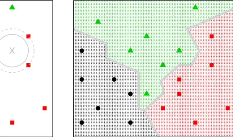
Figure 1 illustrates how the k-nearest neighbor classi…cation works with a small arti…cial dataset containing three classes. The left-hand side of Figure 1 illustrates the nearest neighbors of two new data points based on Euclidean distance. The amount of nearest neighbors k is assumed to be either 1 or 3. For two example locations marked with X, the solid gray circle shows the one nearest neighbor and
dashed circle illustrates the neighbors when k equals three. The right-hand side of Figure 1 shows the decision boundary for this arti…cial data when k equals one.
l l l l l l l X X l l l l l l l lllllllllllllllllllllllllllllllllllllllllllllllllllllllllllllllllllllllllllllllllllllllllllllllllllllllllllllll lllllllllllllllllllllllllllllllllllllllllllllllllllllllllllllllllllllllllllllllllllllllllllllllllllllllllllllll lllllllllllllllllllllllllllllllllllllllllllllllllllllllllllllllllllllllllllllllllllllllllllllllllllllllllllllll lllllllllllllllllllllllllllllllllllllllllllllllllllllllllllllllllllllllllllllllllllllllllllllllllllllllllllllll lllllllllllllllllllllllllllllllllllllllllllllllllllllllllllllllllllllllllllllllllllllllllllllllllllllllllllllll lllllllllllllllllllllllllllllllllllllllllllllllllllllllllllllllllllllllllllllllllllllllllllllllllllllllllllllll lllllllllllllllllllllllllllllllllllllllllllllllllllllllllllllllllllllllllllllllllllllllllllllllllllllllllllllll lllllllllllllllllllllllllllllllllllllllllllllllllllllllllllllllllllllllllllllllllllllllllllllllllllllllllllllll lllllllllllllllllllllllllllllllllllllllllllllllllllllllllllllllllllllllllllllllllllllllllllllllllllllllllllllll lllllllllllllllllllllllllllllllllllllllllllllllllllllllllllllllllllllllllllllllllllllllllllllllllllllllllllllll lllllllllllllllllllllllllllllllllllllllllllllllllllllllllllllllllllllllllllllllllllllllllllllllllllllllllllllll lllllllllllllllllllllllllllllllllllllllllllllllllllllllllllllllllllllllllllllllllllllllllllllllllllllllllllllll lllllllllllllllllllllllllllllllllllllllllllllllllllllllllllllllllllllllllllllllllllllllllllllllllllllllllllllll lllllllllllllllllllllllllllllllllllllllllllllllllllllllllllllllllllllllllllllllllllllllllllllllllllllllllllllll lllllllllllllllllllllllllllllllllllllllllllllllllllllllllllllllllllllllllllllllllllllllllllllllllllllllllllllll lllllllllllllllllllllllllllllllllllllllllllllllllllllllllllllllllllllllllllllllllllllllllllllllllllllllllllllll lllllllllllllllllllllllllllllllllllllllllllllllllllllllllllllllllllllllllllllllllllllllllllllllllllllllllllllll lllllllllllllllllllllllllllllllllllllllllllllllllllllllllllllllllllllllllllllllllllllllllllllllllllllllllllllll lllllllllllllllllllllllllllllllllllllllllllllllllllllllllllllllllllllllllllllllllllllllllllllllllllllllllllllll lllllllllllllllllllllllllllllllllllllllllllllllllllllllllllllllllllllllllllllllllllllllllllllllllllllllllllllll lllllllllllllllllllllllllllllllllllllllllllllllllllllllllllllllllllllllllllllllllllllllllllllllllllllllllllllll lllllllllllllllllllllllllllllllllllllllllllllllllllllllllllllllllllllllllllllllllllllllllllllllllllllllllllllll lllllllllllllllllllllllllllllllllllllllllllllllllllllllllllllllllllllllllllllllllllllllllllllllllllllllllllllll lllllllllllllllllllllllllllllllllllllllllllllllllllllllllllllllllllllllllllllllllllllllllllllllllllllllllllllll lllllllllllllllllllllllllllllllllllllllllllllllllllllllllllllllllllllllllllllllllllllllllllllllllllllllllllllll lllllllllllllllllllllllllllllllllllllllllllllllllllllllllllllllllllllllllllllllllllllllllllllllllllllllllllllll lllllllllllllllllllllllllllllllllllllllllllllllllllllllllllllllllllllllllllllllllllllllllllllllllllllllllllllll lllllllllllllllllllllllllllllllllllllllllllllllllllllllllllllllllllllllllllllllllllllllllllllllllllllllllllllll lllllllllllllllllllllllllllllllllllllllllllllllllllllllllllllllllllllllllllllllllllllllllllllllllllllllllllllll lllllllllllllllllllllllllllllllllllllllllllllllllllllllllllllllllllllllllllllllllllllllllllllllllllllllllllllll lllllllllllllllllllllllllllllllllllllllllllllllllllllllllllllllllllllllllllllllllllllllllllllllllllllllllllllll lllllllllllllllllllllllllllllllllllllllllllllllllllllllllllllllllllllllllllllllllllllllllllllllllllllllllllllll lllllllllllllllllllllllllllllllllllllllllllllllllllllllllllllllllllllllllllllllllllllllllllllllllllllllllllllll lllllllllllllllllllllllllllllllllllllllllllllllllllllllllllllllllllllllllllllllllllllllllllllllllllllllllllllll lllllllllllllllllllllllllllllllllllllllllllllllllllllllllllllllllllllllllllllllllllllllllllllllllllllllllllllll lllllllllllllllllllllllllllllllllllllllllllllllllllllllllllllllllllllllllllllllllllllllllllllllllllllllllllllll lllllllllllllllllllllllllllllllllllllllllllllllllllllllllllllllllllllllllllllllllllllllllllllllllllllllllllllll lllllllllllllllllllllllllllllllllllllllllllllllllllllllllllllllllllllllllllllllllllllllllllllllllllllllllllllll lllllllllllllllllllllllllllllllllllllllllllllllllllllllllllllllllllllllllllllllllllllllllllllllllllllllllllllll lllllllllllllllllllllllllllllllllllllllllllllllllllllllllllllllllllllllllllllllllllllllllllllllllllllllllllllll lllllllllllllllllllllllllllllllllllllllllllllllllllllllllllllllllllllllllllllllllllllllllllllllllllllllllllllll lllllllllllllllllllllllllllllllllllllllllllllllllllllllllllllllllllllllllllllllllllllllllllllllllllllllllllllll lllllllllllllllllllllllllllllllllllllllllllllllllllllllllllllllllllllllllllllllllllllllllllllllllllllllllllllll lllllllllllllllllllllllllllllllllllllllllllllllllllllllllllllllllllllllllllllllllllllllllllllllllllllllllllllll lllllllllllllllllllllllllllllllllllllllllllllllllllllllllllllllllllllllllllllllllllllllllllllllllllllllllllllll lllllllllllllllllllllllllllllllllllllllllllllllllllllllllllllllllllllllllllllllllllllllllllllllllllllllllllllll lllllllllllllllllllllllllllllllllllllllllllllllllllllllllllllllllllllllllllllllllllllllllllllllllllllllllllllll lllllllllllllllllllllllllllllllllllllllllllllllllllllllllllllllllllllllllllllllllllllllllllllllllllllllllllllll lllllllllllllllllllllllllllllllllllllllllllllllllllllllllllllllllllllllllllllllllllllllllllllllllllllllllllllll lllllllllllllllllllllllllllllllllllllllllllllllllllllllllllllllllllllllllllllllllllllllllllllllllllllllllllllll lllllllllllllllllllllllllllllllllllllllllllllllllllllllllllllllllllllllllllllllllllllllllllllllllllllllllllllll lllllllllllllllllllllllllllllllllllllllllllllllllllllllllllllllllllllllllllllllllllllllllllllllllllllllllllllll lllllllllllllllllllllllllllllllllllllllllllllllllllllllllllllllllllllllllllllllllllllllllllllllllllllllllllllll lllllllllllllllllllllllllllllllllllllllllllllllllllllllllllllllllllllllllllllllllllllllllllllllllllllllllllllll lllllllllllllllllllllllllllllllllllllllllllllllllllllllllllllllllllllllllllllllllllllllllllllllllllllllllllllll lllllllllllllllllllllllllllllllllllllllllllllllllllllllllllllllllllllllllllllllllllllllllllllllllllllllllllllll lllllllllllllllllllllllllllllllllllllllllllllllllllllllllllllllllllllllllllllllllllllllllllllllllllllllllllllll lllllllllllllllllllllllllllllllllllllllllllllllllllllllllllllllllllllllllllllllllllllllllllllllllllllllllllllll lllllllllllllllllllllllllllllllllllllllllllllllllllllllllllllllllllllllllllllllllllllllllllllllllllllllllllllll lllllllllllllllllllllllllllllllllllllllllllllllllllllllllllllllllllllllllllllllllllllllllllllllllllllllllllllll lllllllllllllllllllllllllllllllllllllllllllllllllllllllllllllllllllllllllllllllllllllllllllllllllllllllllllllll lllllllllllllllllllllllllllllllllllllllllllllllllllllllllllllllllllllllllllllllllllllllllllllllllllllllllllllll lllllllllllllllllllllllllllllllllllllllllllllllllllllllllllllllllllllllllllllllllllllllllllllllllllllllllllllll lllllllllllllllllllllllllllllllllllllllllllllllllllllllllllllllllllllllllllllllllllllllllllllllllllllllllllllll lllllllllllllllllllllllllllllllllllllllllllllllllllllllllllllllllllllllllllllllllllllllllllllllllllllllllllllll lllllllllllllllllllllllllllllllllllllllllllllllllllllllllllllllllllllllllllllllllllllllllllllllllllllllllllllll lllllllllllllllllllllllllllllllllllllllllllllllllllllllllllllllllllllllllllllllllllllllllllllllllllllllllllllll lllllllllllllllllllllllllllllllllllllllllllllllllllllllllllllllllllllllllllllllllllllllllllllllllllllllllllllll lllllllllllllllllllllllllllllllllllllllllllllllllllllllllllllllllllllllllllllllllllllllllllllllllllllllllllllll lllllllllllllllllllllllllllllllllllllllllllllllllllllllllllllllllllllllllllllllllllllllllllllllllllllllllllllll lllllllllllllllllllllllllllllllllllllllllllllllllllllllllllllllllllllllllllllllllllllllllllllllllllllllllllllll lllllllllllllllllllllllllllllllllllllllllllllllllllllllllllllllllllllllllllllllllllllllllllllllllllllllllllllll lllllllllllllllllllllllllllllllllllllllllllllllllllllllllllllllllllllllllllllllllllllllllllllllllllllllllllllll lllllllllllllllllllllllllllllllllllllllllllllllllllllllllllllllllllllllllllllllllllllllllllllllllllllllllllllll lllllllllllllllllllllllllllllllllllllllllllllllllllllllllllllllllllllllllllllllllllllllllllllllllllllllllllllll lllllllllllllllllllllllllllllllllllllllllllllllllllllllllllllllllllllllllllllllllllllllllllllllllllllllllllllll lllllllllllllllllllllllllllllllllllllllllllllllllllllllllllllllllllllllllllllllllllllllllllllllllllllllllllllll lllllllllllllllllllllllllllllllllllllllllllllllllllllllllllllllllllllllllllllllllllllllllllllllllllllllllllllll lllllllllllllllllllllllllllllllllllllllllllllllllllllllllllllllllllllllllllllllllllllllllllllllllllllllllllllll lllllllllllllllllllllllllllllllllllllllllllllllllllllllllllllllllllllllllllllllllllllllllllllllllllllllllllllll lllllllllllllllllllllllllllllllllllllllllllllllllllllllllllllllllllllllllllllllllllllllllllllllllllllllllllllll lllllllllllllllllllllllllllllllllllllllllllllllllllllllllllllllllllllllllllllllllllllllllllllllllllllllllllllll lllllllllllllllllllllllllllllllllllllllllllllllllllllllllllllllllllllllllllllllllllllllllllllllllllllllllllllll lllllllllllllllllllllllllllllllllllllllllllllllllllllllllllllllllllllllllllllllllllllllllllllllllllllllllllllll lllllllllllllllllllllllllllllllllllllllllllllllllllllllllllllllllllllllllllllllllllllllllllllllllllllllllllllll lllllllllllllllllllllllllllllllllllllllllllllllllllllllllllllllllllllllllllllllllllllllllllllllllllllllllllllll lllllllllllllllllllllllllllllllllllllllllllllllllllllllllllllllllllllllllllllllllllllllllllllllllllllllllllllll lllllllllllllllllllllllllllllllllllllllllllllllllllllllllllllllllllllllllllllllllllllllllllllllllllllllllllllll lllllllllllllllllllllllllllllllllllllllllllllllllllllllllllllllllllllllllllllllllllllllllllllllllllllllllllllll lllllllllllllllllllllllllllllllllllllllllllllllllllllllllllllllllllllllllllllllllllllllllllllllllllllllllllllll lllllllllllllllllllllllllllllllllllllllllllllllllllllllllllllllllllllllllllllllllllllllllllllllllllllllllllllll lllllllllllllllllllllllllllllllllllllllllllllllllllllllllllllllllllllllllllllllllllllllllllllllllllllllllllllll lllllllllllllllllllllllllllllllllllllllllllllllllllllllllllllllllllllllllllllllllllllllllllllllllllllllllllllll lllllllllllllllllllllllllllllllllllllllllllllllllllllllllllllllllllllllllllllllllllllllllllllllllllllllllllllll lllllllllllllllllllllllllllllllllllllllllllllllllllllllllllllllllllllllllllllllllllllllllllllllllllllllllllllll lllllllllllllllllllllllllllllllllllllllllllllllllllllllllllllllllllllllllllllllllllllllllllllllllllllllllllllll lllllllllllllllllllllllllllllllllllllllllllllllllllllllllllllllllllllllllllllllllllllllllllllllllllllllllllllll lllllllllllllllllllllllllllllllllllllllllllllllllllllllllllllllllllllllllllllllllllllllllllllllllllllllllllllll lllllllllllllllllllllllllllllllllllllllllllllllllllllllllllllllllllllllllllllllllllllllllllllllllllllllllllllll lllllllllllllllllllllllllllllllllllllllllllllllllllllllllllllllllllllllllllllllllllllllllllllllllllllllllllllll lllllllllllllllllllllllllllllllllllllllllllllllllllllllllllllllllllllllllllllllllllllllllllllllllllllllllllllll lllllllllllllllllllllllllllllllllllllllllllllllllllllllllllllllllllllllllllllllllllllllllllllllllllllllllllllll lllllllllllllllllllllllllllllllllllllllllllllllllllllllllllllllllllllllllllllllllllllllllllllllllllllllllllllll lllllllllllllllllllllllllllllllllllllllllllllllllllllllllllllllllllllllllllllllllllllllllllllllllllllllllllllll lllllllllllllllllllllllllllllllllllllllllllllllllllllllllllllllllllllllllllllllllllllllllllllllllllllllllllllll lllllllllllllllllllllllllllllllllllllllllllllllllllllllllllllllllllllllllllllllllllllllllllllllllllllllllllllll lllllllllllllllllllllllllllllllllllllllllllllllllllllllllllllllllllllllllllllllllllllllllllllllllllllllllllllll lllllllllllllllllllllllllllllllllllllllllllllllllllllllllllllllllllllllllllllllllllllllllllllllllllllllllllllll l l l l l l l l l l l l l l l l l l l l l l l l l l l l l l l l l l l l l l l l l l l l l l l l l l l l l l l l l l l l l l l l l l l l l l l l l l l l l l l l l l l l l l l l l l l l l l l l l l l l l l l l l l l l l l l l l l l l l l l l l l l l l l l l l l l l l l l l l l l l l l l l l l l l l l l l l l l l l l l l l l l l l l l l l l l l l l l l l l l l l l l l l l l l l l l l l l l l l l l l l l l l l l l l l l l l l l l l l l l l l l l l l l l l l l l l l l ll ll ll ll l l l l l l l l ll ll ll l l l l l l l l l l l l l l l l ll ll lll lll l l l l l l l l l l l l l l l l l l l l lllllll lllllll ll ll l l ll ll lll lll ll ll l l lll lll l l ll ll l l ll ll l l l l l l lll lll ll ll ll ll lll lll l l l l lll lll lll lll ll ll lll lll lllll lllll lll lll ll ll l l llll llll l l ll ll ll ll l l l l llll llll ll ll l l l l ll ll l l l l ll ll lllll lllll l l ll ll l l ll ll l l ll ll ll ll l l l l lll lll l l l l l l l l llll llll l l l l l l lll lll lll lll ll ll ll ll ll ll llll llll l l ll ll lll lll lll lll ll ll l l llllllll llllllll l l lll lll llll llll l l l l ll ll l l ll ll l l lll lll l l ll ll lll lll lll lll ll ll l l llll llll l l llllll llllll l l llll llll llll llll l l ll ll llll llll ll ll lll lll l l l l l l lll lll lll lll ll ll l l l l l l l l l l l l l l l l l l l l l l l l l l l l l l l l l l l l l l l l l l l l l l l l l l l l l l l l l l l l l l l l l l l l l l l l l l l l l l l l l l l l l l l l l l l l l l l l l l l l l l l lllllllllllllllllllllllllllllllllllllllllllll l l l l l l l l l l l l l l l l l l l l l l l l l l l l l l l l l l l l l l l l l l l l l l l l l l l l l l l l l l l l l l l l l l l l l l l l l l l l l l l l l l l l l l l l l l l l l l l l l l l l l l l l l l ll ll ll ll l l l l lll lll ll ll l l l l ll ll ll ll ll ll l l lll lll l l l l lllll lllll ll ll l l lll lll l l l l ll ll lllll lllll lll lll l l ll ll lll lll llll llll ll ll l l l l l l l l ll ll l l l l lll lll ll ll l l l l ll ll l l ll ll lll lll l l l l ll ll l l l l lllllll lllllll l l l l l l l l l l l l l l l l l l l l l l l l l l l l l l l l l l l l l l l l l l l l l l l l l l l l l l l l l l l l l l l l l l l l l l l l l l l l l l l l l l l l l l l l l l l l l l l l l l l l l l l l l l l l l l l l l l l l l l l l l l l l l l l l l l l l l l l l l l l l l l l l l l l l l l l l l l l l l l l l l l l l l l l l l l l l l l l l l l l l l l l l l l l l l l l l l l l l l l l l l l l l l l l l l l l l l l l l l l l l l l l l l l l l l l l l l l l l l l l l l l l l l l l l l l l l l l l l l l l l l l l l l l l l l l l l l l l l l l l l l l l l l l l l l l l l l l l l l l l l l lllllllllllllllllllllllllllllllllllllllllllllllllllllllllllllllllllllllllllllllllllllllllllllllllllll
Figure 1: k-Nearest neighbor classi…cation
Thek-nearest neighbor classi…cation is used as a benchmark method in this thesis because it is fairly easy to …netune. The only tuning parameter of the method is the amount of neighbors k. Larger values of k lead to smoother and less detailed decision boundaries. Despite its simplicity k-nearest neighbor has shown success in di¤erent kinds of classi…cation problems such as handwritten digits or satellite image scenes. Since the features in the dataset could have a variety of di¤erent scales each feature is typically re-scaled to have mean zero and variance equal to one. (Hastie, Tibshirani & Friedman, 2009).
2.2.2 Gradient boosting
The classi…cation algorithm called adaboost was …rst introduced by Freund and Schapire (1996). For a long time the classi…cation ability of the adaboost algorithm remained controversial. This was until Friedman, Hastie and Tibshirani (2000) cre-ated a statistical framework for the boosting procedure and showed how the adaboost algorithm …ts an additive logistic regression model. The more general gradient boost-ing algorithm was discovered as Friedman (2001) introduced the connection to numer-ical optimization in function space. The more general gradient boosting algorithm can be used for both classi…cation and regression problems.
In gradient boosting the goal is to …nd the function minimizing the expected loss of some predetermined loss function
^
F(xt 1) = arg min
F(xt 1)
E[L(yt; F(xt 1))]:
In order to keep the notation fairly simple let us consider the binary classi…cation problem, where yt 2 f0;1g and L(yt; F(xt 1)) is the binomial deviance. With the
multinomial response variable presented in equation (3) a separate function is esti-mated for each class, which complicates the notation.
Gradient boosting is an ensemble method, where the possibly very complex …nal model is a combination of simple models called base learners.
FM(xt 1) =
M
X
m=1
fm(xt 1) (7)
The base learners f(xt 1) are assumed to belong to some parameterized class of
functions. These could be for example simple linear models, spline functions or regression trees. The base learner used in this study is theJ-terminal node regression tree, which splits the predictor space into J disjoint regions and attaches a constant to each region. Mathematically the J-terminal node regression tree base learner can be written as f(xt 1;fcj; RjgJj=1) = J X j=1 cjI(xt 1 2Rj); (8) wherecj 2R is the functional estimate in region Rj.
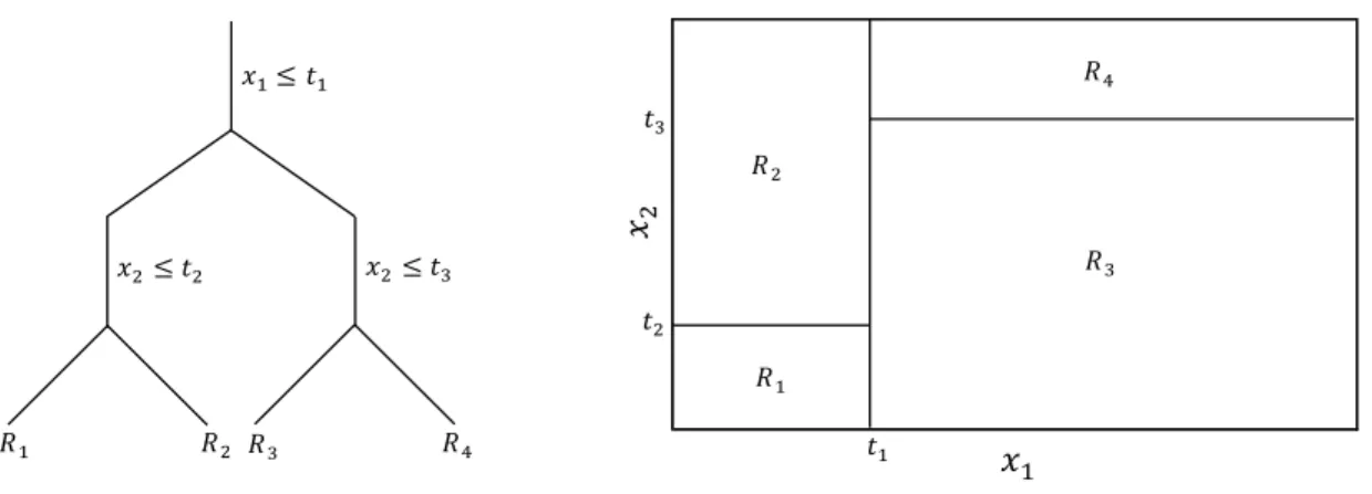
Figure 2 illustrates J-terminal node regression trees graphically and plots a 4-terminal node regression tree and the 4-terminal node regions created by this tree. The left-hand side depicts the classical tree shape. Each of the three split points is a function of the splitting variables and split locations. The right-hand side of Figure 2 shows the terminal node regions fRjg4j=1 and the split locationsftlg3l=1in a
Figure 2: 4-terminal node regression tree
The …nal ensemble in equation (7) is estimated in a greedy stagewise fashion using a method called forward stagewise additive modeling. The estimation of a gradient boosting model is described in Algorithm 1. The algorithm starts with an initial value, which is a simple constant based on the considered loss function. At each iteration m of the gradient boosting algorithm a new base learner function which best …ts the negative gradient of the loss function is selected and added to the current ensemble Fm 1. With the J-terminal node regression tree in equation (8)
as the base learner this corresponds to …nding the J non-overlapping terminal node regions fRjmgJj=1 using a least squares criterion. After …nding the terminal node
regions the functional estimates^cjm are obtained in a simple minimization problem. The current ensemble Fm 1 is then updated with the functional estimates before
calculating the pseudo responses y~t for the next round of the algorithm.
Algorithm 1 Gradient boosting using J-terminal node regression trees
F0(xt 1) = arg minN1 N X t=1 L(yt; ) for m 1 to M do: ~ yt = @L(yt;F(xt 1)) @F(xt 1) F(x t 1)=Fm 1(xt 1) ; t = 1; ::; N
estimate fRjmgJj=1 using the least squares criterion
^ cjm = arg min cjm X xt 12Rjm L(yt; Fm 1(xt 1) +cjm); j = 1; ::; J
Fm(xt 1) = Fm 1(xt 1) + J P j=1 ^ cjmI(xt 1 2Rjm) end for
Algorithm 1 also illustrates the tuning parameters related to the gradient boosting method. The amount of iterations M and the learning rate 2 ]0;1] control the learning process. Setting M too low can result in under…tting whereas too many repeats can lead to over…tting. Setting the learning rate smaller than one can be seen as a shrinkage strategy as the parameter shrinks each functional estimate towards zero and thereby controls the speed of the learning process. These two parameters are inversely related to each other. A smaller learning rate usually requires more trees to be built (Hastie et al., 2009).
The amount of complexity related to the J-terminal node regression tree base learner function can be controlled by the amount of terminal nodesJ and the amount of observations required at each terminal node region. Requiring more observations in each terminal node region narrows down the amount of potential split points and therefore controls the complexity of each tree. Building larger trees with more terminal nodes results in more complex models but the risk of over…tting also grows. Note from the graphical illustration in Figure 2 that in order to build aJ-terminal node regression treeJ 1split points are needed and the size of the regression tree also controls the amount of interactions allowed between di¤erent predictors. Instead of requiring the exact amount of terminal nodes J some software implementations use the depth of the treeD as a tuning parameter. The depth of the regression tree is the maximum amount of inner nodes between the root and leaf nodes. The depth of the regression tree in Figure 2 for example is two since there are two split points between the root and each leaf node.
Di¤erent subsampling strategies can also be used for reqularization with the gra-dient boosting model. The subsampling is usually done row-wise, where only a certain fraction row of training samples are used when estimating the parameters of
the base learner function at each round of the algorithm. By using row-wise sub-sampling the regression trees at each round tend to be less similar. Additionally column-wise subsampling is also available, where only a certain fraction col of the
available predictors are used at each round of the gradient boosting algorithm. The exact amount of subsampling used both row-wise and column-wise are …netuned using cross-validation.
2.2.3 Random forest
The random forest algorithm of Breiman (2001) has a close connection to both bag-ging and the adaboost classi…cation algorithm. The …nal model with each of these three methods is an ensemble of simple models. The original idea of random forest is to improve the classi…cation ability of bagging by reducing the correlation be-tween each component in the …nal ensemble. This is done by injecting additional randomness when building each component of the …nal model.
Similarly as with boosting the base learner function used at each step of the ran-dom forest algorithm is a tree-based model. Unlike the regression tree presented in equation (8) the base learner with random forest classi…cation algorithm is a classi-…cation tree. The graphical illustration given in Figure 2 holds for the classiclassi-…cation tree as well, but now the functional estimate in each terminal node region of the J-terminal node classi…cation tree is the predicted class
f(xt 1;fCj; RjgJj=1) =
J
X
j=1
CjI(xt 1 2Rj); (9) wherext 1 is a vector of inputs at time t 1and Cj is the predicted class in region Rj:
Instead of …xing the number of terminal nodes J as with gradient boosting the complexity of each tree in the random forest is typically controlled by requiring a certain number of observations at each terminal node. In the random forest algorithm the depth of each tree is increased by adding additional split points for as long as the number of observations in the terminal node is greater than a prespeci…ed constant nmin. This constant is a tuning parameter related to the random forest
algorithm as all the terminal nodes must hold at least nmin data points. Especially
with classi…cation problems the trees in the random forest are often grown to the full size requiring only one observation in each terminal node region. Hastie et al. (2009) argue that letting the trees in the random forest to grow to the maximum size seldom costs much and results in one less tuning parameter.
The power of random forests comes from combining the predictions of many accurate individual trees that are as diverse as possible. In order to make the trees in the random forest ensemble less correlated only a subset of features are considered when new split points are added to the classi…cation tree. Suppose the number of features in the dataset is p then only m (m p) randomly chosen features are
considered as candidates when selecting a new split point. The exact amount m depends on the problem at hand and is treated as a tuning parameter. Especially in problems where the proportion of relevant features in the whole feature set is small, settingm too low may result in poor performance (Hastie et al., 2009).
Similarly as in bagging, a bootstrap sample Z of size N is drawn from the training data at each round b 2 f1; :::; Bg of the algorithm. A new decision tree fb(xt 1; ) is …t using this bootstrap sample, where the parameter vector holds
the parameters of the decision tree presented in equation (9). The split points of this decision tree are found recursively by considering only the m randomly chosen features at each step. The decision tree is grown to the maximum possible size controlled by the parameter nmin, which sets the minimum number of observations
needed in each node of the tree. This process is summarized in Algorithm 2.
Algorithm 2 Random Forest classi…cation
for b 1 to Bdo:
draw a bootstrap sample Z of size N from the training data
create an empty decision tree fb(xt 1 2Z ; =;)
while (the number of observations in some node > nmin) do:
randomly select m variables
pick the best split point among these
split the current node into two daughter nodes
end while
include fb(xt 1; ) in the ensemble Fb
end for
The …nal ensemble in the random forest algorithm is a combination of the indi-vidual trees found in each round b of the algorithm
F(xt 1) = ffb(xt 1; )gBb=1:
The classi…cation of a new data point xN is based on a majority vote between the classi…cations induced by each individual tree
^
Crf(xN) = majority votefC^b(xN)gBb=1;
where C^b(xN) is the predicted class given by the bth decision tree in the random forest ensemble.
2.2.4 Neural networks
Neural networks were originally designed as a tool to model the information process-ing capabilities of the human brain and the earliest attempts go as far as the 1940s (Rojas, 1996). There are a vast amount of neural network models with di¤erent as-sumptions regarding the structure of the network and how information ‡ows through the network. The model used in this thesis is one of the most commonly used neural network models called a single hidden layer feed-forward neural network (Bishop, 2006).
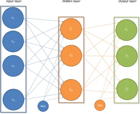
The network consists of three layers which are typically named as the input layer, hidden layer and the output layer. Each layer in a feed-forward network is connected with the subsequent layer through weights as is visualized in Figure 3. The directed edges represent the weights and the direction of information ‡ow in the network.
Input layer Hidden layer Output layer
. . . . . . . . . bias bias
Figure 3: Arti…cial neural network
In general there could be several hidden layers creating a deeper and more complex network. Each unit in the hidden layer of Figure 3 is called a hidden unit since these
are typically unobserved. These hidden units are linear combinations of the input variablesx= (x1; x2; : : : ; xp)
0
followed by a non-linear activation function: Zm =h( 0m+
0
mx); m= 1; :::; M; (10) where 0mis the weight from the bias unit, mis ap 1vector of weights coming into hidden unitZm and h() is the activation function. The sigmoid function is typically used to transform the linear combinations of inputs into a non-linear form. Another common choice for the activation function is the hyperbolic tangent function. Note that the total amount of weights connecting the units in the input layer and the hidden layer is M (p+ 1), where M is the number of units in the hidden layer. The exact amount for M is treated as a tuning parameter of the model.
The …nal output for each class k is formed as a linear combination of the hidden units Z = (Z1; Z2; : : : ; ZM)
0
, which is transformed in the interval [0;1] using the softmax function: Fk=g( 0k+ 0 kZ) = e 0k+ 0 kZ PK l=1e 0l+ 0 lZ ; k = 1; :::; K:
Similarly as in equation (10) 0k is the weight from the bias unit and k is a M 1
vector of weights connecting the units in the hidden layer to the output unit Fk. The optimal weights in the network minimize the considered loss function. In the multinomial classi…cation problem the loss function to be minimized is the sample counterpart of the multinomial deviance shown in equation (6). By denoting the complete set of weights in the network by a weight vector the loss function can be written as L( ;Fk) = N X t=1 K X k=1 I(Rt=k) logFk; (11)
whereFk is the output for classk:The set of weights in the network can be searched using a gradient descent based method called backpropagation. In backpropagation the gradient of the loss function in equation (11) is calculated at each iteration. The weights in the network are then updated according to the direction given by the negative gradient. For a more detailed description of the backpropagation algorithm see e.g. Rojas (1996).
A simple regularization strategy called weight decay has been suggested to avoid over…tting while estimating the optimal weights in the network. In weight decay an
additional penalty term, which penalizes large weights, is added to the loss function presented in equation (11)
~
L( ;Fk) = L( ;Fk) + J( );
where is the weight decay parameter. The penalization function J( ) can take various forms. A common choice is to impose quadratic penalization, where J( ) =
0
(Bishop, 2006). Larger values for thereby shrink the weights towards zero unless traditional backpropagation reinforces the weights. The exact amount of penalization needed is …netuned using cross-validation.
2.2.5 Support vector machines
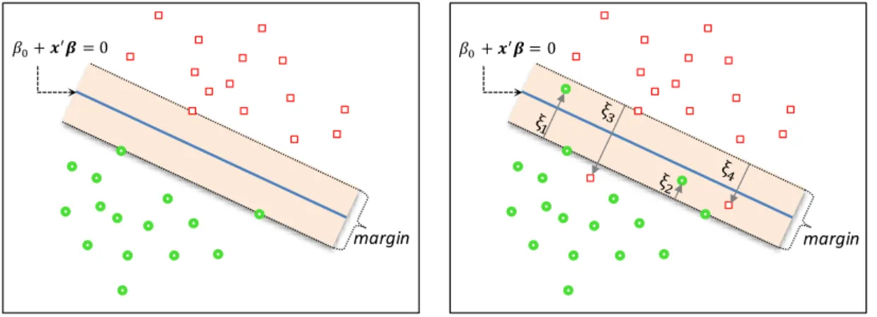
The support vector machines originally presented by Vapnik (1995) can be used for both classi…cation and regression problems. The basic idea and the terminology of support vector machines can be illustrated using a two-class classi…cation problem with a linear decision boundary. The left-hand side of Figure 4 illustrates the case with perfect separability. The right panel in Figure 4 shows the nonseparable case, where some data points are misclassi…ed by the linear decision boundary.
margin margin
Figure 4: Support vector machine
The solid blue line in Figure 4 is the decision boundary separating the two classes F(x) = 0+x0 = 0;
where 0 is a constant term, is a unit vector and x is a p 1 vector of input
variables. For notational reasons let us focus on the binary classi…cation case and denote the binary response as yi 2 f 1;1g; i = 1; :::; N, where i can be associated to time t. The one-against-one method used in this thesis for K-class classi…cation with support vector machines is a direct extension to the binary case as the …nal classi…cation is based on a voting scheme between theK(K 1)=2binary classi…ers constructed for each class pair. For more information on the multiclass classi…cation with support vector machines see e.g. Hsu and Lin (2002).
The goal with support vector machines is to …nd the decision boundary with maximum area on both sides of the boundary also known as the margin
M = 2
k k:
In Figure 4 the dashed lines illustrate the margin and the points located at the dashed lines are known as support vectors. These support vectors play a crucial role when searching for the optimal decision boundary as is shown mathematically later on.
Hastie et al. (2009) show that instead of maximizing the margin the optimization problem can be written in terms of minimizing k k
min
0; k k
s:t: yi( 0+x
0
i ) 1; i= 1; :::; N: (12) The constraint in equation (12) requires each observation to be on the right side of the margin. This constraint does not hold for the nonseparable case shown on the right panel of Figure 4 since some observations are on the wrong side of the margin. For this reason we need to de…ne a vector of slack variables = ( 1; :::; N). For the data points on the correct side of the margin the slack variable is equal to zero and for the misclassi…ed observations i >1. The slack variable is between zero and one when the data point is on the incorrect side of the margin but correctly classi…ed. All of these cases are illustrated on the right-hand side of Figure 4.
In the nonseparable case the constraint in the optimization problem of equation (12) is re-formulated so that some of the observations can be on the incorrect side of the margin. The proportional amount of observations on the wrong side of the margin is bound by requiring the sum of slack variables to be smaller than some
prede…ned constant. The minimization problem then becomes min 0; k k s:t: yi( 0+x 0 i ) 1 i; i= 1; :::; N; i 0; PN i=1 i constant. (13) The convex optimization problem with quadratic objective and linear inequality con-straints in equation (13) can be solved using quadratic programming. The Lagrange primal function can be written as
LP = 1 2k k 2 +C N X i=1 i N X i=1 i[yi( 0+x 0 i ) (1 i)] N X i=1 i i; (14) where C is now inplace of the predetermined constant in equation (13). The para-meters i and i are the Lagrange multipliers. The cost parameter C is a tuning parameter of the procedure and controls how wide the margin is. A larger value ofC puts more emphasis on the points near the decision boundary and requires a tighter margin.
The Lagrange dual objective function can be formulated by plugging the solved parameter values from the …rst order conditions of the primal problem back to equa-tion (14) LD = N X i=1 i 1 2 N X i=1 N X j=1 i jyiyjhxi;xji; (15) where alphas are the Lagrange multipliers from the minimization problem in equation (14) and hxi;xji is the inner product of vectors xi and xj: The dual problem in equation (15) is often easier to solve than the primal (Hastie et al., 2009). Without going into the details of solving the minimization problem the optimal solution turns out to be the following:
^ = N
X
i=1
^iyixi: (16)
Equation (16) shows how the optimal decision boundary is determined by the esti-mated alphas. These estiesti-mated alphas are non-zero only for the observations char-acterized as the support vectors. The support vectors therefore have a direct impact on the location of the decision boundary. It should be noted that the support vectors can also be located inside their margin in the nonseparable case.
So far we have only dealt with linear decision boundaries. To consider non-linear decision boundaries the original input feature space is typically transformed
into an enlarged space using e.g. polynomials or splines since the data could be linearly separable in this higher dimensional feature space. Without specifying the exact transformation the dual problem in equation (15) can be written using these transformed feature vectorsh(xi)
LD = N X i=1 i 1 2 N X i=1 N X j=1 i jyiyjhh(xi); h(xj)i; (17) where hh(xi); h(xj)i is the inner product of the transformed input vectors i and j. The solution to the dual Lagrangian in equation (17) depends on the transformed higher dimensional data only through inner products. Instead of the exact trans-formationh()a kernel function, which computes inner products in the transformed space, is su¢cient. A radial basis function and a dth-degree polynomial are typical choices for the kernel function. The radial basis function can be written as
K(x;xi) = hh(x); h(xi)i= exp( jjx xijj2); (18) where is a tuning parameter related to the radial basis function kernel. The dth-degree polynomial kernel function involves one extra tuning parameter compared to the radial basis kernel presented in equation (18). The degree of the polynomial d needs to be …netuned in addition to a scale parameter s
K(x;xi) = (1 +shx;xii)
d: (19)
The …nal classi…cation in the support vector machine is produced by the following equation ^ G(x) = sign( ^F(x)) =sign( N X i=1 ^iyiK(x;xi) + ^0);
where K(x;xi) is one of the kernel functions presented in equations (18) and (19).
^i and ^0 are the solved coe¢cients from the optimization problem. Similarly as
with the linear decision boundary the coe¢cients ^i are non-zero only for the data points marked as support vectors.
2.3
Previous literature
Forecasting stock prices has attracted a great amount of interest in the recent decades. Especially the machine learning community has been very actively pro-ducing new research in this …eld. The typical research explores if a more ‡exible
machine learning method could improve the predictions by exploiting non-linear re-lationships in the data. The previous literature is quite vast. Atsalakis and Valavanis (2009) produce a comprehensive survey of more than one hundred di¤erent published articles related to stock market forecasting using neural network based techniques alone. For a more recent survey on …nancial forecasting using a variety of di¤er-ent machine learning methods see e.g., Cavalcante, Brasileiro, Souza, Nobrega and Oliveira (2016).
Because of the huge amount of previous research the following literature review focuses on the particular strand of literature where the dependent variable is bi-nary. To the best of our knowledge the multinomial response variable presented in equation (3) has not been considered in previous literature related to the directional prediction of stock returns. The closest alternative can be found in Boonpeng and Jeatrakul (2016), where they compose the daily price information in the stock market into three di¤erent trading signals using technical analysis technique called pivoting. These di¤erent types of trading signals are then predicted using alternative technical analysis indicators as input.
Kara, Boyacioglu and Baykan (2011) compare the performance of arti…cial neural networks (ANN) and support vector machines (SVM) in predicting the daily direction of change in the Istanbul stock exchange. Various technical analysis indicators are used as the input variables. In a very similar study Patel, Shah, Thakkar and Kotecha (2015) forecast the direction of two Indian stock indices and two individual stocks. In addition to ANN and SVM Patel et al. (2015) also consider random forests. The single hidden layer feed-forward network produces slightly more accurate results than the SVM with polynomial kernel in Kara et al. (2011). Patel et al. (2015) reach another conclusion with the Indian data as SVM is seen to outperform ANN. Random forest however provides the most accurate directional predictions for both the indices and individual stocks considered in Patel et al. (2015).
Both Kara et al. (2011) and Patel et al. (2015) conduct a quite extensive grid search to …nd the optimal tuning parameter combinations for each model. The dataset for parameter optimization in both of these studies is randomly selected from the entire dataset. For this reason the actual forecasting results are highly con-troversial, since the models have already seen some of the test data while optimizing the tuning parameters. The fairly high hit ratios above 70 or even above 80 percent are in line with this observation.
Other studies reporting results in favor of using the SVM over the ANN in fore-casting the direction of stock markets are found using data from the Asian markets.
Huang, Nakamori and Wang (2005) forecast the direction of a Japanese stock index using weekly data. Huang et al. (2005) also report impressive hit ratios above 70 percent, but their results are based on a test set consisting of 36 observations only. Kim (2003) use the radial basis function SVM to predict the daily direction of Ko-rean stock exchange using technical analysis indicators as input. SVM is seen to outperform ANN but the di¤erence between these two methods is not statistically signi…cant. The magnitude of the hit ratios reported by Kim (2003) is closer to a true stock market forecasting experiment.
Ballings, den Poel, Hespeels and Gryp (2015) provide a more extensive compari-son of di¤erent machine learning methods in directional prediction of stock returns. They use yearly data for 5767 listed European companies and forecast if the yearly price change of an individual stock in year 2010 is above 35 percent or not. Using such a high threshold to create the binary response variable leads to highly imbal-anced classes. The class imbalance problem is handled by oversampling the majority class.
All the machine learning methods considered in this thesis except for the gradient boosting model (GBM) are included in the model set of Ballings et al. (2015). The family of boosting algorithms is however represented as the adaboost classi…cation algorithm is also studied. Random forest is found to be the top-performer followed by SVM and adaboost based on the median area under the ROC-curve (AUC) among the individual …rms. Krauss et al. (2017) also focus on the performance of individual companies and model if the daily return of a particular stock in the S&P 500 index is above the market return or not. Both random forest and GBM is seen to outperform deep neural networks while a combination of all these models yields the most accurate predictions.
Zhong and Enke (2017) run di¤erent linear and non-linear dimensionality reduc-tion techniques before applying ANN in predicting the direcreduc-tion of the S&P 500 stock market index. The standard linear principal component analysis (PCA) combined with the ANN yields the most accurate predictions and provides important insights into selecting the optimal predictor set. Especially lagged returns, other stock mar-kets, the largest companies in the S&P 500 index and di¤erent exchange rates are considered as in‡uential predictors in the PCA-step.
In a recent study Basak, Kar, Saha, Khaidem and Dey (2019) conduct a direc-tional prediction for ten randomly selected companies included in the S&P 500 index using a variety of di¤erent machine learning models. Before constructing the binary
response variable they smooth the return series using exponential smoothing. This exponential smoothing shifts the focus onto detecting a medium to long-term price trend instead of the daily direction of change in market prices.
Di¤erent technical analysis indicators derived from the smoothed return series are used as the input for models. The model set considered by Basak et al. (2019) include all the models used in this thesis except for k-nearest neighbors. Random forest yields the best long-term trend forecasts before GBM and ANN. The selection for tuning parameters is fairly novel and the results should be viewed with healthy criticism. For example the worst performing method is the SVM, which is trained using the linear kernel function only.
3
Data and model setup
3.1
Data
The dataset used in the empirical section of this thesis covers daily returns of the S&P 500 stock market index from the beginning of the 1990s to the end of 20182. The goal of the empirical analysis is to study a wide spectrum of di¤erent variables that could be used for prediction using the maximum amount of daily data available. With such a high frequency as daily returns the potential predictor variables are mostly based on di¤erent types of …nancial market data.
As was seen in the previous section technical analysis indicators have been the most common choice for the input variables of di¤erent machine learning methods (see e.g., Kim, 2003; Basak et al., 2019). In technical analysis di¤erent types of indi-cators are calculated using the historical price or return information from the stock market. Benchmark yields and di¤erent interest rate spreads from the corporate and government bond markets have also been extensively studied with both daily and monthly data (see e.g., Zhong and Enke, 2017; Nyberg and Pönkä, 2016). Interest rates express the tightness of the monetary policy set by the Federal Reserve. Di¤er-ent types of interest rate spreads re‡ect market expectations regarding the upcoming economic activity or the riskiness of the corporate sector for example.
Lagged stock returns and returns from other stock markets are another commonly used alternative (see e.g., Zhong and Enke, 2017). A less studied predictor group is the volatility in di¤erent markets. A recent study by Becker & Leschinski (2018) shows that the VIX-index, which is often called the fear factor of stock markets, can also be a viable alternative. As with Zhong and Enke (2017) di¤erent exchange rates and commodities indices are also considered as potential features to be used for prediction in this thesis. The appreciation (or depreciation) of the dollar relative to other currencies a¤ects the foreign trade and international ‡ow of funds to the U.S. Variables related to the state of the macroeconomy are found to be important predictors when predicting monthly stock returns (Nyberg, 2011). Unfortunately the majority of the macroeconomic information is not available with daily frequency.
Table 1 summarizes the input variables using seven di¤erent categories. A short description and an illustrative example are shown from each category. The full
2After deriving and lagging the predictor variables the exact time period is 12.2.1990
predictor set and the exact transformations for each predictor can be found in the appendix.
Table 1: Predictor groups
Group Description Example
Stock market S&P 500 price infor-mation, Returns from other stock markets
Lagged returns, Re-turns from DAX or FTSE
Interest rates Government and cor-porate benchmark yields
3-month T-bill, Term spread
Exchange rates The appreciation of dollar relative to other currencies
Dollar/British Pound, major currencies in-dex
Commodities Information from the commodities market
Copper, Oil, Gold, Silver
Volatility Volatility in the stock and bond markets
VIX-index, MOVE-index
Technical analysis Indicators derived from price or return information
Relative strength in-dex
Macro Information regarding the macroeconomy
ADS-index
The total amount of di¤erent predictors studied in this thesis is 37. Following the approach of Krauss et al. (2017) various lag lengths of the predictors are also considered. Lag lengths beyond ten trading days are found to be uninformative in the preliminary analysis using the model selection capability of the gradient boosting machine3. By considering the lagged predictors from the previous ten trading days the full predictor set consists of 370 di¤erent inputs (37 10). Only data points (days) with information available for each predictor are considered. For this reason
predictor variables utilizing market data outside the U.S. is kept minimal because of the individual holiday periods in each country. After leaving out the data points with missing values the …nal dataset includes 6686 daily observations.
From the machine learning methods considered in this thesis only the tree-based classi…ers gradient boosting machine and random forest are capable of handling such a large predictor set. Both of these methods are able to perform model selection simultaneously with estimation as new split points are introduced for the tree-based base learners. Other methods end up easily over…tting the data with a large predictor set and therefore a reduced dataset is needed. A smaller predictor set is built using a combination of prior knowledge and the results from the tree-based methods.
Both GBM and random forest select the VIX-index as the single most in‡uential predictor4. For the random forest model each of the ten most in‡uential inputs are di¤erent lag lengths of the VIX-index, whereas GBM includes six lags of VIX in the top-10. Di¤erent technical analysis indicators are also considered as important predictors by both models. The best performing technical analysis indicators are the stochastic oscillator (StochK), moving average convergence divergence (MACD) and Williams %R (Rperc)5. The ranking of these indicators are slightly di¤erent for the two methods.
In addition to these the spread between the daily high and low stock prices is selected by both models. GBM also ranks the corporate interest rate spread among the ten most in‡uential predictors. The results from the principal component analysis by Zhong and Enke (2017) are in favor of using the lagged stock returns and international stock returns. Lagged stock returns from the S&P 500 and the returns from the German stock index are thereby also included in the reduced dataset.
The reduced dataset includes six inputs which are the VIX-index, MACD-indicator, spread between daily high and low prices, corporate interest rate spread, lagged stock returns and returns from the DAX-index. The data from the previous three trading days are used for each predictor. The total amount of inputs in the reduced dataset is thereby 18 (6 3). Several other choices for both the composition of predictors and lag lengths were also considered.
4For more information about the relative in‡uence measure see Breiman (2001) and Friedman
(2001).
3.2
Tuning parameter optimization
Each of the machine learning methods considered in this thesis involve free parame-ters that a¤ect the …nal output of the model. Often the parameparame-ters can a¤ect the results quite dramatically as is the case with neural networks for example (Zhang, Patuwo & Hu, 1998). These parameters are usually called tuning parameters since it is up to the end user to …netune the optimal parameters for the particular learning task.
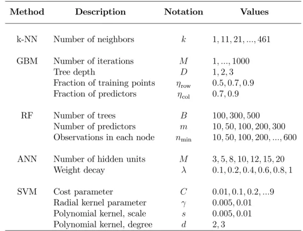
Table 2 summarizes the tuning parameters of the machine learning methods stud-ied in this thesis. A brief description and the notation used for the tuning parameter in the methodological part of this thesis is shown in Table 2. The last column il-lustrates the considered parameter values. It should be noted that for each method a wider grid search has been conducted in order to …nd a suitable range for each parameter. Only this smaller interval is depicted in Table 2.
Table 2: Tuning parameters for each method
Method Description Notation Values
k-NN Number of neighbors k 1;11;21; :::;461
GBM Number of iterations M 1; :::;1000
Tree depth D 1;2;3
Fraction of training points row 0:5;0:7;0:9
Fraction of predictors col 0:7;0:9
RF Number of trees B 100;300;500
Number of predictors m 10;50;100;200;300
Observations in each node nmin 10;50;100;200; :::;600
ANN Number of hidden units M 3;5;8;10;12;15;20
Weight decay 0:1;0:2;0:4;0:6;0:8;1
SVM Cost parameter C 0:01;0:1;0:2; :::9
Radial kernel parameter 0:005;0:01
Polynomial kernel, scale s 0:005;0:01
Because the number of di¤erent machine learning methods considered in this the-sis is quite large some simpli…cations have been done in order to keep the parameter search feasible. Additional …netuning would be available for several methods. There are for example alternative distance measures for the k-NN method and di¤erent learning algorithms for the ANN-model. Following the approach of Hastie et al. (2009) the learning rate in the gradient boosting machine algorithm is set as small as possible. The learning rate is held …xed at a value of 0.001. For computational reasons the parameter search is restricted to the parameter values presented in Table 2.
The performance of each model speci…cation is evaluated using the validation ac-curacy produced by theK-fold cross-validation procedure. InK-fold cross-validation the training sample is split into K independent folds. Each of these K folds is used as a hold-out test set once, while the remaining K 1folds are used for estimating the model. This process is repeated for each fold and the validation accuracy is the average accuracy produced by theK independent folds
CVAcc = 1 K K X k=1 Acck;
where K is the amount of folds and Acck is the obtained accuracy when the data points of foldk are used as an independent test set.
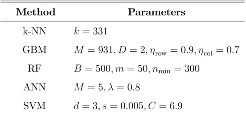
10-fold cross-validation is used to estimate the optimal tuning parameters for each method. Table 3 shows the parameter optimization results and depicts the optimal tuning parameter combination for each method.
Table 3: Final model speci…cations
Method Parameters k-NN k = 331 GBM M = 931; D = 2; row = 0:9; col = 0:7 RF B = 500; m = 50; nmin = 300 ANN M = 5; = 0:8 SVM d= 3; s= 0:005; C = 6:9
Relatively restricted models are chosen in the cross-validation procedure as can be seen in Table 3. This is not very surprising as the noisy stock market data combined with a complex model can easily lead to overlearning the training data. The limitations in allowed ‡exibility can be seen for each method. For example, quite a large number of nearest neighbors are used while classifying each data point and the tree-based methods GBM and RF seem to favor quite shallow trees. A fairly small amount of neurons are used in the hidden layer of an ANN-model combined with quite a heavy penalization through the weight decay parameter. The polynomial kernel of degree 3 is used for the support vector machine and the cost parameter is rather small, which results in a wider margin and also supports the …nding of restricted models.
The low amount of hidden neurons reported in Table 3 for the ANN is of similar magnitude as the parameter value selected using trial-and-error in Zhong and Enke (2017). The results from a tuning parameter optimization procedure in Kara et al. (2011) also favor the use of a polynomial kernel over the radial basis function for the SVM. The polynomial kernel of degree three is the optimal choice when forecasting the direction of the Turkish stock market as well (Kara et al., 2011). Based on prior knowledge Krauss et al. (2017) end up with the same tree depth for the GBM-model as reported in Table 3.
4
Empirical results
4.1
Estimation results
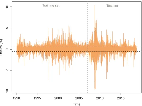
The complete data sample covering the time period from 12.2.1990 to 5.10.2018 is split into two parts. The training set contains data before the year 2007 and is used for training and validating the models. The test set covering the rest of the data is used as an independent test set to evaluate how well each method performs on a completely unseen dataset. Therefore roughly 58 percent of the complete dataset is used for training and the remaining 42 percent for testing. The test set thus contains 3899 daily observations.
Figure 5 visualizes the daily returns of the S&P 500 index. The horizontal dashed lines show the upper and lower quartiles of the return, which are used as the thresh-olds in equation (3) to create the multinomial response variable. The vertical gray dashed line illustrates the split into training and testing datasets.
1990 1995 2000 2005 2010 2015 -10 -5 0 5 10 Time Retur n (%)
Training set Test set
In order to keep the test set completely independent, the upper and lower quartiles of the return are calculated using only the training data6. The benchmark accuracy for the training and validation is one half as the majority class contains …fty percent of the observations. In the test set there are slightly more observations coming from the majority class and the strategy of always predicting the majority class yields the accuracy of 0.526. This should be used as the benchmark accuracy when evaluating the prediction results for the test set.
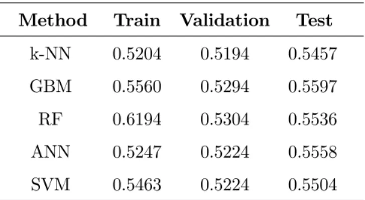
The estimation results for each machine learning method are presented in Table 4. The …rst column shows the considered method while the next three columns give the classi…cation accuracies for the training, validation and test sets.
Table 4: Estimation results
Method Train Validation Test
k-NN 0.5204 0.5194 0.5457
GBM 0.5560 0.5294 0.5597
RF 0.6194 0.5304 0.5536
ANN 0.5247 0.5224 0.5558
SVM 0.5463 0.5224 0.5504
The results indicate signi…cant return forecastability as the classi…cation accura-cies for the training and validation sets are well above the benchmark of one half for each method. In terms of the training and validation accuracies the results are in favor of using the tree-based methods gradient boosting and random forest, which can utilize the full predictor set. The relatively high training accuracy for the ran-dom forest model stands out from the rest, however the validation accuracy is only slightly higher than for GBM. ANN and SVM have a similar validation performance. The simplicity of the nearest neighbor algorithm has led to the lowest training and validation accuracies.
The classi…cation results for the test set indicate how well the models generalize to new data. The observation of return predictability seems to hold even when test-ing on an unseen dataset as the accuracies for each method are well above the test set
6The upper and lower quartiles for the training set are
f 0:4989%;0:5755%g whereas the quartiles for the entire dataset aref 0:4656%;0:5723%g.
benchmark performance. The ranking between the machine learning methods based on the classi…cation accuracies for the test set is slightly di¤erent from the ranking obtained using the accuracies for the training set. While GBM still outperforms the other machine learning methods random forest reaches only the third highest test accuracy as neural networks show better generalization ability. The fairly large deviance between the training and testing results for the random forest raises ques-tions of potential over…tting. A similar observation can be made when comparing the generalization capabilities of ANN and SVM. The SVM model has better training accuracy but results in slightly lower generalization performance.
4.2
Economic in‡uence
Leitch and Tanner (1991) argue that a model performing well from a statistical point of view does not necessarily imply economic pro…tability, especially when trading costs are taken into account. In order to evaluate the ability to gain economic pro…ts a real-life trading simulation is conducted. Our trading simulation is similar to those in Pesaran and Timmermann (1995) and Leung et al. (2000) for example. The classi…cation patterns are turned into a trading strategy, which depends on the current ( ^Rt+1) and previous forecasted class ( ^Rt), as can be seen in Table 5.
Table 5: Trading strategy ^
Rt
1 2 3
1 Stay out Sell Sell ^
Rt+1 2 Buy Hold Hold
3 Buy Hold Hold
Table 5 shows how the multinomial response variable enables a richer set of possible trading strategies compared to the more commonly studied binary response case. In a traditional market timing setup as presented in Pesaran and Timmermann (1995) an asset allocation decision is made between investing in stocks or in bonds. With the daily trading frequency the returns from investing in the bond market are fairly low and we only consider the options of staying fully invested in stocks or not.