Machine Learning Methodologies for Interpretable Compound Activity Predictions

Machine Learning Methodologies for

Interpretable Compound Activity

Predictions

Kumulative Dissertation

zur Erlangung des Doktorgrades (Dr. rer. nat.)

der Mathematisch-Naturwissenschaftlichen Fakultät

der Rheinischen Friedrich-Wilhelms-Universität Bonn

vorgelegt von

Raquel Rodríguez Pérez

aus Barcelona, Spanien

Bonn

November, 2019

Angefertigt mit Genehmigung

der Mathematisch-Naturwissenschaftliche Fakultät

der Rheinischen Friedrich-Wilhelms-Universität Bonn

1. Referent: Univ.-Prof. Dr. rer. nat. Jürgen Bajorath

2. Referent: Univ.-Prof. Dr. rer. nat. Holger Fröhlich

Tag der Promotion: 20.02.20

Abstract

Machine learning (ML) models have gained attention for mining the

phar-maceutical data that are currently generated at unprecedented rates and

po-tentially accelerate the discovery of new drugs. The advent of deep learning

(DL) has also raised expectations in pharmaceutical research. A central task

in drug discovery is the initial search of compounds with desired biological

ac-tivity. ML algorithms are able to find patterns in compound structures that

are related to bioactivity, the so-called structure-activity relationships (SARs).

ML-based predictions can complement biological testing to prioritize further

experiments. Moreover, insights into model decisions are highly desired for

fur-ther validation and identification of activity-relevant substructures. However,

the interpretation of complex ML models remains essentially prohibitive. This

thesis focuses on ML-based predictions of compound activity against multiple

biological targets. Single-target and multi-target models are generated for

rele-vant tasks including the prediction of profiling matrices from screening data and

the discrimination between weak and strong inhibitors for more than a hundred

kinases. Moreover, the relative performance of distinct modeling strategies is

systematically analyzed under varying training conditions, and practical

guide-lines are reported. Since explainable model decisions are a clear requirement

for the utility of ML bioactivity models in pharmaceutical research, methods

for the interpretation and intuitive visualization of activity predictions from

any ML or DL model are introduced. Taken together, this dissertation presents

contributions that advance in the application and rationalization of ML models

for biological activity and SAR predictions.

Contents

Motivation

1

1

Introduction

3

2

Prediction of Compound Profiling Matrices Using Machine

Learning

27

Introduction . . . .

27

Publication . . . .

29

Summary . . . .

41

3

Multitask Machine Learning for Classifying Highly and Weakly

Potent Kinase Inhibitors

43

Introduction . . . .

43

Publication . . . .

45

Summary . . . .

55

4

Influence of Varying Training Set Composition and Size on

Sup-port Vector Machine-Based Prediction of Active Compounds

57

Introduction . . . .

57

Publication . . . .

59

Summary . . . .

67

5

Relative Performance of Multitask Deep Learning and

Ran-dom Forest Classification on the Basis of Varying Amounts of

Training Data

69

Introduction . . . .

69

Publication . . . .

71

Summary . . . .

79

6

Support Vector Machine Classification and Regression

Prior-itize Different Structural Features for Binary Compound

Ac-tivity and Potency Value Prediction

81

Publication . . . .

83

Summary . . . .

93

7

Interpretation of Compound Activity Predictions from

Com-plex Machine Learning Models Using Local Approximations

and Shapley Values

95

Introduction . . . .

95

Publication . . . .

97

Summary . . . 115

8

Conclusions

117

List of abbreviations

1D, 2D, 3D

One-, two-, three-dimensional

ADMET

Absorption, distribution, metabolism, excretion, and toxicity

CNN

Convolutional neural network

DL

Deep learning

DNN

Deep neural network

DT

Decision tree

ECFP

Extended-connectivity fingerprint

HTS

High-throughput screening

MACCS

Molecular access system

ML

Machine learning

MMP

Matched molecular pair

MT

Multitask

QSAR

Structure-activity relationship

QSPR

Structure-property relationship

RECAP

Retrosynthetic combinatorial analysis procedure

RF

Random forest

SAR

Structure-activity relationship

SMILES

Simplified molecular-input line-entry system

SPR

Structure-property relationship

ST

Single-task

SV

Support vector

SVM

Support vector machines

SVR

Support vector regression

Tc

Tanimoto coefficient

Motivation

Machine learning (ML) and, more recently, deep learning models have gained

attention in pharmaceutical research due to the emergence of “big data” at

different levels including medicinal chemistry.

The exploration of

structure-activity relationships (SARs) represents a critically important task in medicinal

chemistry and is essential for the development of novel bioactive compounds.

ML models are suitable for leveraging and mining the nearly exponential

in-creasing amounts of compound activity data that are currently generated and

published.

_{ML enables qualitative or quantitative SAR modeling and the}

sub-sequent prediction of compound bioactivity from structural representations.

The identification of active compounds by computational methods plays an

im-portant role in drug discovery and complements high-throughput screening.

Virtual screening protocols can be implemented using ML so that experimental

testing is prioritized on the basis of model predictions. Some small molecules

specifically interact with multiple targets, which might cause higher drug

effi-cacy or undesired side effects. Therefore, multi-target predictions or activity

profile predictions are currently a fundamental challenge of high interest.

_With

the rise of deep learning techniques, the potential benefit of deep neural

net-works (DNNs) for bioactivity modeling requires a systematic assessment.

Hence, prediction scenarios that mimic real-life screening or introduce

challeng-ing test systems are required.

Moreover, despite being decisive for ML model

quality, the influence of the nature of training data on activity predictions is

still an underinvestigated issue. Finally, interpretable ML models would

pro-vide insights into structural patterns driving changes in predicted compound

activity and enable the extraction of SAR information. However, ML-based

predictions are difficult to rationalize, especially for DNNs, which are often

considered as “black boxes”.

_{Thus, insights into complex model decisions}

are essentially prohibitive which often hinders the practical use of ML models

in pharmaceutical research.

In this thesis, ML models are systematically

de-veloped, analyzed, and rationalized for the prediction of compound bioactivity

against multiple targets. More specifically, the main objectives of this thesis

are: (i) the application and comparison of ML strategies for the prediction of

compound activity profiles, (ii) the study of the influence of training set

condi-tions on model performance, and (iii) the improvement of the interpretability

of ML-based compound activity predictions.

Thesis outline

This dissertation consists of eight chapters structured as follows.

Chapter 1

presents an introduction to drug discovery and important applications of ML

models in pharmaceutical research, with emphasis on compound activity

predic-tions.

Chapter 2

to

Chapter 7

contain six original publications representing the

main work of this thesis.

Chapter 2

reports the development and benchmark

of ML approaches for the prediction of compound profiling matrices.

Chapter

3

presents the ML-based classification of weakly and highly potent inhibitors

against a panel of kinases. In

Chapter 4

, guidelines for training set size and

composition are derived for support vector machines models applied to activity

predictions.

Chapter 5

investigates the relative performance of single-target

ML and multi-target DNNs for the prediction of multiple assays from

screen-ing data.

Chapter 6

systematically studies the feature importance in support

vector machines models for activity and potency prediction. In

Chapter 7

, a

method for the interpretation of activity predictions from any ML algorithm

is introduced and validated. Finally,

Chapter 8

summarizes and discusses the

major findings of this thesis.

Chapter 1

Introduction

Drug discovery

The ultimate goal of pharmaceutical research is the identification of novel

compounds with desired properties for the treatment of a given disease. Drug

discovery research broadly includes (i) target identification, (ii) hit discovery,

and (iii) lead optimization.

_{A biological target, generally a protein, is}

in-volved in a dysfunctional biological process and its modulation alleviates

symp-toms or modifies the disease state.

_{The identification of putative}

therapeu-tic targets implies the understanding of the connection between the molecular

mechanisms and the disease. Identified targets are subsequently validated to

confirm the relationship between target and disease.

Currently, two major

groups of drug targets are G protein-coupled receptors and kinases.

Next,

a search for active compounds (or hits) that bind to the target and modify

its function is pursued. Hit identification mainly relies on high-throughput

screening (HTS) technologies, which include miniaturized and robotized assay

platforms that test the activity of thousands or hundreds of thousands of

com-pounds against a biological target in a short time.

_{Once hits are found, lead}

compounds or classes that serve as starting points are obtained and undergo

multi-parametric optimization to improve other desired properties.

At this

stage, absorption, distribution, metabolism, excretion, and toxicity (ADMET)

properties of lead compounds are characterized and improved.

Compound

op-timization consists of many cycles of synthesis of close analogs to improve the

properties based on small structural modifications. After these discovery

search stages, a promising drug candidate must satisfy pre-clinical and clinical

development requirements. Only if clinical evaluation in human cohorts is

suc-cessful, a drug could be approved by the pharmaceutical regulatory agencies.

Figure 1

schematizes the main phases of drug discovery and clinical

develop-ment of a new drug, which take an average time of 12 years and are very costly

(

∼

$2

.

6

billion according to a recent estimation).

_{Moreover, pharmaceutical}

R&D investment has considerably increased during the last years without a

pos-itive impact on the number of discovered drugs,

_{which reflects the existence}

of some issues and bottlenecks.

Clinical

development

Pre-clinical

development

Lead

optimization

Hit

discovery

Target

identification

Figure 1: Drug discovery and development. An overview of the main stages in drug discovery and development is shown.

The role of computational approaches

A variety of computational approaches have been introduced to improve

and accelerate drug discovery.

Bioinformatics and chemoinformatics focus on

data processing and thus differ from computational biology, which

mathemat-ically models and simulates biological systems, and computational chemistry,

which has its foundation in theoretical and quantum chemistry. Bioinformatics

typically studies “omic”-data such as genomics or proteomics, whereas

chemoin-formatics focuses on small molecules and their role as ligands.

_{As such, this}

thesis covers chemoinformatic approaches for drug discovery. Chemoinformatics

was firstly defined as

“the mixing of information resources to transform data into

information, and information to knowledge, for the intended purpose of making

better decisions faster in the area of drug lead identification and optimization”

.

Bio- and chemoinformatics disciplines, which contribute to pharmaceutical

re-search with considerable overlap, have been continuously evolving both with

novel algorithms and applications.

Machine learning in pharmaceutical research

Machine learning (ML) approaches have been established as essential tools

for bio- and chemoinformatics.

_{There is a need for new data mining methods}

able to cope with growing amounts of heterogeneous data sets, which offer many

opportunities but are difficult to analyze and utilize. ML belongs to the

spec-trum of artificial intelligence methods, which are closely linked to the big data

era and have currently become a hot topic in many areas including

pharmaceuti-cal research.

ML uses statistical pattern recognition algorithms that enable

a system to learn from experience and subsequently make predictions about

new data. Supervised ML can be used to predict discrete or continuous

vari-ables, whereas unsupervised methods are mainly used for exploratory analysis,

visualization and clustering. Particularly, deep learning (DL) is a subdiscipline

of ML that encompasses non-linear methods which can model complicated

re-lationships between input and output data using low-level representations.

DL has surpassed standard ML methods in disciplines such as computer vision

and natural language processing.

Consequently, DL has also experienced

an increasing interest in pharmaceutical research.

Both ML and DL have

encountered applications across all stages of drug discovery and development.

Models have yielded accurate predictions for distinct bioinformatics tasks

including target

_{or biomarker discovery.}

_{Some studies have shown the}

potential of ML methods to distinguish between cancer and non-cancer targets

on the basis of gene expression

_{or predict the suitability of targets for drug}

development from physicochemical, structural and geometric features of

pro-tein cavities.

_{ML has also been used to predict drug response across cell lines}

on the basis of gene expression data.

DL offers opportunities to deal with

large amounts of single-cell RNA sequencing data, reduce dimensionality, and

identify cell-specific biomarkers or characterize cell states and types.

Using

pre-clinical data, ML models also enabled the identification of gene signatures

for patient sub-groups that respond better to drug treatment.

_{In addition,}

pathology image processing has experienced a considerable improvement

af-ter the introduction of DL methodologies which prevent the need of manually

identifying “handcrafted” task-specific features.

_{DL models have been used}

for the classification and segmentation of microscopy images

as well as the

identification of breast cancer regions in a large data set of pathology images.

Chemoinformatics has also benefited from ML modeling.

Recently,

computer-aided synthesis planning has become a relevant application

_and

some studies have focused on the prediction of the major reaction products

given a set of reactant molecules

_{or the conditions of organic synthesis}

reac-tions.

_{For the task of novel chemical structures generation or}

_{de novo}

_design,

a variety DL methods, such as variational autoencoder,

_{generative adversarial}

networks,

recurrent neural networks,

and deep reinforcement learning,

have been recently proposed. These approaches seem promising for generating

compounds with desired properties, but the chemical diversity and validity of

output samples are currently still debated.

Since the chemical structure of a compound determines its properties,

medic-inal chemistry studies structure-property relationships (SPRs), which can be

modeled using ML.

_{Distinct ML methods}

_{including deep neural networks}

(DNNs)

_{have been applied to quantitative SPRs (QSPRs) modeling. One of}

the most relevant compound properties is biological activity. Compound

activ-ity predictions generally help at the hit identification stage, whereas QSPRs for

potency or ADMET properties are often considered in lead optimization.

Compound activity predictions

The understanding and analysis of structure-activity relationships (SARs)

is a central goal in medicinal chemistry and drug discovery. Since the big data

era has arrived in medicinal chemistry, influenced by HTS and combinatorial

chemistry,

_{ML has become a method of choice to mine chemical information}

and find molecules with desired bioactivity. Going beyond volume, compound

activity data fulfills other big data-related terms such as heterogeneity,

confi-dence, complexity, variability, and veracity.

_{In this context, ML-based activity}

predictions have found some relevant applications.

Virtual screening

A key application of bioactivity prediction is virtual screening (VS), which

complements HTS through a prioritization of experimental testing.

_Despite

the numerous experiments performed by HTS, few bioactive compounds are

found and hit rates are typically below 1-2%.

Thus, VS aims at selecting

small numbers of potentially active compounds from in-house, commercial or

virtual combinatorial libraries.

Aside from ligand-based methods, which use compound activity data for

pre-dictions and are at the heart of the research presented in this thesis, methods

relying on structural information about the targets present alternative relevant

approaches.

_{Structure-based VS requires the three-dimensional (3D) structure}

of the target macromolecule, which can be obtained by X-ray crystallography

or nuclear magnetic resonance spectroscopy.

_{Molecular docking is the most}

popular structure-based approach, which aims to find the preferred orientation

or binding conformation of a ligand to a receptor through a computationally

intensive optimization.

Docking uses a mechanism to explore the space of

protein-ligand geometries and a scoring function to rank the possibilities.

Re-cently, ML methods have been proposed to score protein-ligand interactions,

including convolutional neural networks.

On the other hand, ligand-based VS requires active compound data and

of-ten becomes the method of choice when 3D structures are not available.

Sim-ilarity searching is the classical approach for the detection of active compounds

based on known ligand data,

but ML models have become widely used.

Dif-ferent studies have shown the ability of ML to identify structurally distinct

com-pounds with similar activity (task also known as scaffold hopping),

which is a

pre-requisite for successful VS.

In retrospective studies, Doddareddy

et al.

trained linear discriminant analysis and support vector machines (SVM)

mod-els on the basis of compound fingerprints and detected blockers of potassium

ion channels potentially leading to cardiotoxic effects.

_{VS approaches have}

also shown successful results in prospective applications

_{including a}

sup-port vector regression model that detected new inhibitors of histone deacetylase

1

and a naïve Bayes model which identified inhibitors of phosphatidylinositol

3-kinase.

With the integration of experimental and computational screening, ML

models trained on the basis of biological screening data might select less but

“smarter” experiments for the next round.

_{Active learning approaches have}

been developed for VS,

_{where the model iteratively selects compounds to}

test and is updated with the acquired data. The choice of the next

experi-ments can rely on exploration (i.e. selection of useful data for model building)

or exploitation (i.e. selection of compounds likely to be active) strategies.

Nevertheless, HTS and VS integration is challenging due to the inherent noise,

experimental variance, large data volumes, diversity of chemical classes,

possi-ble presence of distinct binding modes, as well as strong statistical imbalance

between hits and inactive compounds in HTS data.

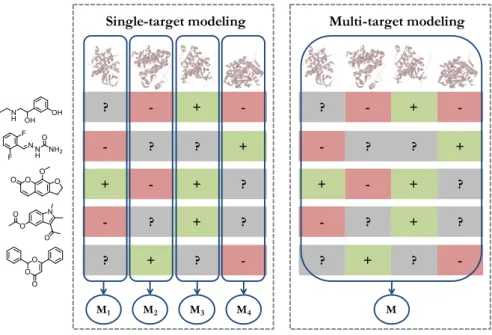
Multi-target activity

ML models can be trained to predict multi-target activities of compounds,

also referred to as activity profiles.

Figure 2

illustrates compound

activ-ity profiles for exemplary compounds and schematizes the difference between

single-target and multi-target modeling. An important limitation of the “one

target, one drug” paradigm is the non-consideration of multi-target activity

at early stages of the drug discovery.

_{The ability of small molecules to}

specifically engage in interactions with multiple receptors is the molecular

ba-sis of polypharmacology. Therapeutic polypharmacology achieves a stronger

therapeutic effect by simultaneously targeting distinct points in a particular

pathogenic process.

_{and is promising to combat complex diseases, such as}

cancer or neurological disorders, that might require a more elaborate

pharma-cological action.

However, multi-target activities might also be responsible for

undesired side effects. The ultimate objective of chemogenomics is fully

char-acterizing the interactions between all available chemical ligands and biological

targets, which is practically unfeasible.

_{Hence, chemogenomics focuses on}

the exploration and navigation of limited ligand-target spaces, typically on the

basis of protein families or related receptors. Since compound bioactivity

pro-files would enable a better prioritization of drug candidates, activity prediction

against multiple targets is a highly relevant topic.

_{However, the optimization}

of multi-target SARs is complicated.

_{Some approaches have been proposed}

such as SVM modeling with distinct kernel functions that account for protein

sequence, structure, and hierarchy information for compound-target binding

prediction.

_{Moreover, the performance of chemogenomics models that predict}

the interaction or non-interaction of protein-ligand pairs has been assessed

and compared to individual SAR models.

_{Recently, DL architectures have}

also been applied to multi-target activity predictions.

v + ? - -? - ? + + + - ? + - ? ? ? ? + -+ ? - -? - ? + + + - ? + - ? ? ? ? + -M M1 M2 M3 M4

Single-target modeling Multi-target modeling

Figure 2: Single-target and multi-target modeling. A compound-target matrix with activity annotations (red: inactive, green: active, gray: unknown or missing) is schematized. Single-target (left) and multi-target (right) models predict compound bioactivity for one or multiple targets, respectively.

Orphan or novel targets

In principle, SAR modeling is not applicable to targets for which no actives

are known, so-called orphan targets. However, some approaches have been

im-plemented to overcome this limitation. The most simplistic method relies on

ligands from homologous targets.

_{More sophisticated approaches have been}

proposed including SVM with specialized target-ligand kernels or linear

com-binations of SVM models.

Furthermore, chemogenomics models that

dis-criminate between compound-target interacting or non-interacting pairs allow

ligand binding prediction for orphan or novel targets.

As stated above, ML and DL models are attractive for drug discovery

be-cause they enable handling large amounts of heterogeneous and noisy data. ML

strategies have been successfully validated for many prediction tasks.

How-ever, a “hype” is typically encountered when new technologies are first

intro-duced to drug discovery

_{and this also applies to artificial intelligence methods.}

Hence, the real benefits of DL approaches remain unknown for many desired

tasks. ML applications are often burdened by the lack of interpretability and

rationalization of model success and failure, which is further aggravated in DL,

given its extreme black box nature.

Even accurate DL models are often

compromised in different application scenarios.

Therefore, if model decisions

cannot be understood, the practical use of ML might be limited despite its

undisputed potential.

Structure-activity relationships modeling

In addition to activity prediction, ML models statistically relate compound

structure patterns to biological activity.

_{For SAR and quantitative SAR}

(QSAR) modeling, compounds are numerically represented by a feature vector

and a learning algorithm maps these feature vectors to activity.

_In

particu-lar, the chosen molecular representation defines the theoretical chemical space

under study and the model accounts for similarity measures in such space.

Molecular representations

Following graph theory concepts, chemical structures can be represented

as graphs, in which atoms and bonds correspond to nodes and edges,

respec-tively.

_{Linear notations such as the simplified molecular-input line-entry}

sys-tem (SMILES)

_{or the IUPAC international chemical identifier (InChI)}

allow efficient storage of large compound data sets and can be converted to the

molecular graph.

_{For predictive modeling, descriptors of molecular structure}

and properties are typically calculated either from the one-dimensional (1D)

molecular formula, two-dimensional (2D) graph or 3D conformation.

Some

examples of distinct complexity are molecular weight or atom counts (1D),

con-nectivity indexes or structural fragments (2D), and van der Waals volume or

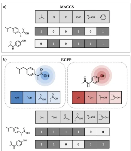
v OH OH O_OH O OH OH OH O N H OH OH OH OH OH O OH O OH OH OH 1 1 1 1 0 0 0 1 1 0 1 1 ECFP OH O OH 1 0 0 1 0 1 0 0 1 1 1 1 C C F O N H OH N MACCS O OH O N H OH b) a) O OH

Figure 3: Molecular fingerprints. Schematic visualization of MACCS (a) and ECFP (b) for two exemplary compounds. These molecular fingerprints codify the presence (1) or absence (0) of chemical substructures or patterns. MACCS includes pre-defined structural keys or substructures, and ECFP encodes atom circular environments for each compound. In (b) atom environments are only generated for one exemplary atom.

spatial pharmacophores (3D).

_{Molecular 2D fingerprints are a well-known}

rep-resentation that encodes the presence or absence of chemical substructures or

patterns in a binary vector. Structural keys codify pre-defined chemical patterns

or substructures of a fixed length.

_{Molecular access system (MACCS) keys are}

a prominent example consisting of 166 bit positions,

which provide an

easy-to-rationalize fingerprint as shown in

Figure 3a

. The extended-connectivity

fingerprint (ECFP) is a hashed fingerprint that encodes circular atom

environ-ments up to a given diameter, as illustrated in

Figure 3b

.

Therefore, ECFPs

are more general than structural keys and result in a higher-dimensional

rep-resentation. ECFP length is variable by design, but it can be transformed to

a fixed-length vector through modulo mapping (folding). Recently, DL

archi-tectures that directly learn from the compound SMILES

or 2D graphs have

been reported,

_{which alleviate the feature engineering process.}

Structural similarity

SAR modeling is based on the “similarity property principle” which states

that

“compounds with similar chemical structure share similar properties”

.

Structural similarity has been intensively studied in chemoinformatics for the

comparison of compounds and their properties, mainly bioactivity.

Never-theless, a clear and consistent similarity assessment by computational methods

is complicated due to the subjective nature of the concept.

_{The matched}

molecular pair (MMP) formalism is a chemically intuitive way to determine

analogs.

_{A pair of compounds forming an MMP only differs by a structural}

modification at a single site, as shown in

Figure 4

. Therefore, an MMP consists

of a common core or key fragment, and a chemical transformation. The

frag-mentation required for MMP generation can be based on retrosynthetic

combi-natorial analysis procedure (RECAP) rules.

RECAP fragmentation is

com-putationally efficient and accounts for synthetic accessibility. RECAP-MMPs

can be organized in molecular networks, where nodes and edges represent

com-pounds and MMP relationships, respectively. As a result, each disjoint cluster

of the network is considered a unique analog series.

v S N N N N Cl H N Br S N N N N Cl H N

Figure 4: MMP concept. Exemplary MMP formed by two compounds with common core that only differ by a chemical transformation (highlighted in blue).

There are different metrics that can be used to quantify similarity (i.e.

1-distance) on the basis of molecular representations. Tanimoto coefficient (Tc)

or Jaccard index is very popular for 2D fingerprints, and is given by (1) for two

compound fingerprints.

_Here

_A

_and

_B

_{represent the sets of features present}

in either of the two molecules.

Tc

(

A, B

) =

|A

∩

B

|

|A

∪

B

|

=

|A

∩

B

|

|A|

+

|B| − |A

∩

B|

(1)

Similarity searching

Similarity searching is the classic ligand-based approach for identifying new

active compounds.

_{Following the similarity property principle, fingerprint}

similarity based on the Tc (or another metric) is used as an indicator of

ac-tivity.

In particular, database molecules with unknown activity are ranked

according to their decreasing similarity to an active reference molecule. Despite

its simplistic nature, this approach is often effective providing an early

enrich-ment of actives on the top of the ranking.

_{A variety of extensions of standard}

similarity searching have been introduced to improve performance including the

combination of multiple searches (data fusion) or fingerprint modification.

Some exemplary methods are Turbo similarity searching,

_{consensus bit}

scaling,

_{and conditional correlated Bernoulli model.}

_{With the advent}

of ML models, traditional similarity searching has mainly found its application

in descriptive statistics, exploratory analysis and fast extensive calculations,

such as large-scale VS.

Machine learning models for SAR analysis and

prediction

The influence of chemical modifications on compound activity can be

mod-eled using ML either in a qualitative (classification) or quantitative (regression)

fashion. Based on their structural fingerprints, compounds are projected onto

a well-defined

m

-dimensional chemical space. In such a feature space, similar

molecules map closely together and ML models aim at recognizing differential

patterns that enable accurate predictions. Formally, a supervised ML model

relates a feature vector

x

= (

x

, ..., x

)

∈ X

to an output label

y

, where

y

=

{

+1

,

−

1

}

for binary classification and

y

∈

_R

for regression, through a

func-tion

f

so that

f

(

x

) =

y

. The ML model attempts to minimize the expected test

error, which can be decomposed into bias, variance and a constant irreducible

noise term, as shown in (2) for a test instance

x

with label

y

. Bias refers to

the error introduced by approximating a real-life problem using a much simpler

model. Variance measures the variability or sensitivity of the prediction

func-tion to a particular choice of data. Clearly, a successful model simultaneously

achieves low bias and variance.

E

y

−

f

ˆ

(

x

)

=

h

Bias

f

ˆ

(

x

)

i

+

h

Var

f

ˆ

(

x

)

i

+

(2)

Underfitting Optimum Overfitting

Figure 5: Optimization of model complexity. The prediction error in training and internal validation sets depends on model complexity. Very simple models, which generally have high bias and low variance, are not able to model the data properly (underfitting). Complex models are often characterized by low bias and high variance and model peculiarities of training data (overfitting). The optimum model complexity is obtained by minimizing the internal validation error.

As illustrated in

Figure 5

, model complexity determines the bias and

vari-ance trade-off, which reflects the need of complexity optimization when models

rely on tuning hyper-parameters.

_{Simple models might be unable to capture}

the underlying patterns (underfitting) and complex models tend to fit the

inher-ent noise of training data (overfitting). Validation is an essinher-ential part of model

building aiming at complexity optimization as well as performance estimation.

Thus, it requires three data partitions: training set (model fitting), internal

validation set (model selection), and test or external validation set (model

as-sessment).

_{Cross-validation might be utilized to account for different splits}

or folds and make better use of the available data.

Naïve Bayes

Naïve Bayes is a binary classifier that relies on the Bayes’ theorem.

The

term “naïve” refers to the assumption of conditional feature independence.

De-spite this simplification, naïve Bayes classifiers have been successfully applied in

problems with correlated features.

_{Bayes’ theorem is used to determine the}

probability that a compound

x

belongs to class

y

, i.e.

P

(

y|

x

)

. The likelihood

function

P

(

x

|y

)

plays a central role. It can be estimated from the training set

and related to the posterior probability through the Bayes’ theorem (3).

P

(

y|

x

) =

P

(

x

|y

)

P

(

y

)

P

(

x

)

(3)

P

(

y

)

is the prior, i.e. either the known class probability distribution or

its estimation over the training set, and

P

(

x

)

refers to the evidence, which

acts as a normalization constant. Class likelihoods require an event model for

feature distributions and, for binary fingerprints, features follow a multivariate

Bernoulli distribution. For test predictions, the class with maximum likelihood

estimate for the observed data

x

will be selected, as shown in (4).

y

= argmax

ˆ y∈Y

P

(ˆ

y|

x

)

(4)

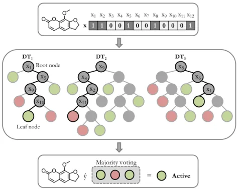
Random forest

A random forest (RF) consists of an ensemble of decorrelated decision trees

(DTs) that elicit variance reduction.

_{A DT is a non-parametric method that}

infers a sequence of binary decision rules to split training data into subsets with

better class separation. Splitting starts from the root (or top) node into child

nodes using rules built on the basis of compound features. DT is a recursive

partitioning method where each child node might in turn split until a stopping

criterion is reached. As illustrated in

Figure 6

, non-leaf nodes represent the

decision rules, edges are possible outcomes, and the predominant class on the

leaf nodes determines the prediction. A tree path from the root to the terminal

node directly indicates the chain of feature-based decisions. DTs can capture

complex interaction structures in the data and have a low bias, but it comes at

the expense of high variance.

DT₁ DT₂ DT₃ x 1 1 0 0 1 0 0 1 0 0 0 1 x3 x1 x2 x4 x5 x6 x7 x8 x9x10x11x12 ŷ Majority voting = Active x1 x5 x9 x10 x9 x8 x2 x11 x8 x6 x1 Root node Leaf node

Figure 6: Principles of RF modeling. A compound with fingerprintxis predicted by a RF model with three DTs. Each non-leaf node represents a decision rule based on a feature (xm). The tree path from the root to the leaf node is highlighted in black. The color of leaf

nodes indicates the predicted label, e.g. active (green) or inactive (red). The final prediction forxis given by a consensus across individual tree predictions.

The classification and regression trees or CART algorithm

constructs DTs

using feature thresholds yielding minimal Gini impurity values. This criterion

encourages the formation of regions with high proportions of data assigned to

one class,

_{and becomes zero when all instances in a node belong to the same}

class.

G

in a node

τ

is formally defined by (5), where

C

refers to the total

number of classes and

p

to the probability of selecting a sample from class

c

.

G

(

τ

) =

C

X

c=1

p

(1

−

p

)

(5)

RF builds a collection of individual DTs using random samples with

replace-ment from the training set, which is known as bagging or bootstrap

aggregat-ing. Furthermore, RF randomly selects a feature set for node splitting (feature

bagging) to prevent DTs relying on the same strong predictors.

These two

bagging strategies decorrelate the trees and introduce variability within the

ensemble model.

_{Final predictions are driven by a consensus across trees.}

RF model achieves reduced variance without increasing the bias of individual

models.

Support vector machines

Classification

The SVM algorithm was initially proposed for binary classification. The

SVM classifier attempts to find a hyperplane

H

=

{

x

|h

w

,

x

i

+

b

= 0

}

, defined

by a normal vector

w

and a bias

b

that separates the positive and negative

classes.

For that purpose, SVM maximizes the margin, i.e. the distance

between the closest training instances from each class and the hyperplane.

These training instances are called support vectors (SVs). The hard-margin

(or maximum margin) hyperplane can be obtained by minimizing the distance

from

H

to the SVs of each class. However, said minimization problem has no

solution when data is not separable by a linear function. Slack variables (

ξ

) are

added to derive a soft-margin hyperplane that enables training errors.

_To

al-low limited numbers of training compounds to map inside the margin or on the

incorrect side of the hyperplane, the minimization problem can be formulated

as indicated in (6).

minimize:

1

2

k

w

k

+

C

X

ξ

subject to:

y

(

h

w

,

x

i

+

b

)

≥

1

−

ξ

with

ξ

≥

0

∀i

(6)

The cost or regularization hyperparameter

C

balances the magnitude of

per-mitted training errors and the margin maximization. Small

C

values tolerate

larger errors, whereas large cost factors lead to a complex model. The primal

optimization problem can be expressed in a dual form using Lagrange

multi-pliers

α

, and the solution yields the normal vector of the hyperplane in (7).

Training examples with non-zero

α

coefficients represent the SVs and solely

determine the hyperplane position. These data points lie on the edge, within

the margin or even on the incorrect side of the hyperplane. The binary SVM

classification is schematized in

Figure 7

.

w

=

X

i

α

y

x

(7)

Once the hyperplane is derived, test data are projected into the feature

space. A ranking can be obtained using the real value

g

(

x

) =

P

i

α

y

h

x

,

x

i

+

b

,

which geometrically corresponds to sliding the hyperplane from the most distant

data point on the positive half space toward the negative side.

_{Test instances}

can be classified according to the side of the plane on which they fall, i.e.

f

(

x

) =

sgn

(

g

(

x

))

, which means that compounds with

f

(

x

) = +1

will be

assigned to the positive class (e.g. active) and

f

(

x

) =

−

1

to the negative class

(e.g. inactive).

Support vector machines (SVM) Support vector regression (SVR)

x1 x2 x1 x2 Margi n ε-tube

Figure 7: Principles of SVM and SVR modeling. In SVM (left), a hyper-plane is generated for binary classification by margin maximization. The goal is differentiating between active (green) and inactive (red) compounds. In SVR (right), a regression function is derived for real value prediction. The gradient from light to dark blue indicates increasing numerical values (e.g. potency). SVs are represented by a black circle and lie within the margin (SVM) or outside the-tube (SVR).

Regression

Support vector regression (SVR) is an extension of the SVM algorithm for

real value predictions.

_{In this case, SVR aims at mapping}

_x

_{as close as}

possi-ble to their real label

y

by deriving a function of the form

f

(

x

) =

h

w

,

x

i

+

b

.

Tolerated differences from observed and predicted values of training data are

at most

. However, slack variables are introduced to allow larger positive and

negative deviations (

ξ

, ξ

) from the so-called

-tube.

In SVR, the

hyperpa-rameter

C

also controls the relaxation of error minimization problem and thus

penalizes large slack variables. Analogously to classification, the optimization

problem is formulated in (8) and can be solved using Lagrangian reformulation,

giving the final regression function in (9).

minimize:

1

2

k

w

k

₊

_C

X

(

ξ

+

ξ

)

subject to:

y

− h

w

,

x

i −

b

≤

+

ξ

∀i

h

w

,

x

i

+

b

−

y

≤

+

ξ

∀i

with

ξ

, ξ

≥

0

(8)

f

(

x

) =

X

(

α

−

α

)

h

x

,

x

i

+

b

(9)

In SVR, SVs are the training data points that have either positive

α

or

α

.

SVs lie on the

-tube or outside of it and are the only training data used for the

prediction of new test examples.

Figure 7

illustrates the generation of a SVR

model.

Kernel trick

For nonlinear data that cannot be accurately modeled in the feature space

X

, the scalar product

h·,

·i

can be replaced by a kernel function

K

(

·,

·

)

.

Conceptually, the kernel function transfers the scalar product to a higher

di-mensional space

W

in which the data might be linearly separated, as shown in

Figure 8

. The advantage is that the non-linear mapping

φ

:

X → W

does not

need to be explicitly computed. The generation of the hyperplane or regression

function only depends on SVs and not on the dimension of the input space,

which allows calculations in a higher dimensional space. A variety of kernel

functions exist including, among others, the Gaussian or radial basis function

kernel and the polynomial kernel. In addition, the Tanimoto kernel expression

is shown in (10) for two compounds with fingerprints

x

and

x

. This kernel

function is based on the Tc and widely used in chemoinformatics.

K

(

x

,

x

) =

h

x

,

x

i

h

x

,

x

i

+

h

x

,

x

i − h

x

,

x

i

(10)

The kernel trick allows non-linear SVM and SVR models but confers “black

box” character to the models.

Input space

𝓧

Higher dimensional space

𝓗

Mapping

𝜙

x

x

x

x

x

Figure 8: Kernel trick SVM applies a non-linear mapping (φ) to project molecular rep-resentations into a higher-dimensional (W) space and enable a linear separation, when it is not possible in the original feature or input space (X).

Deep learning

Deep neural networks

Feedforward deep neural networks (DNNs) are a series of functional

transfor-mations given by a collection of connected units that are organized in sequential

layers.

_{Units in a layer act in parallel. These units are also referred to as}

neurons or basis functions. DNNs need to be constituted by at least an input

layer, two hidden layers, and an output layer.

_{Each neuron receives inputs}

from units in the previous layer and computes its activation value, representing

a vector-to-scalar function. The DNN schematic in

Figure 9

illustrates how

each input to a node is modified by a unique set of weights and biases, thus

giving unique combinations per activation. In particular, the neuron applies a

nonlinear activation function to the weighted sum of its inputs to generate its

output.

The activation

a

j

of neuron

j

in layer

l

is given by (11), where

σ

is

the activation function;

w

jk

indicates the weights at the hidden unit

j

of layer

l

;

a

are the activations from the previous layer;

b

j

is the bias of the neuron;

and the sum is over all neurons

k

in the layer

(

l

−

1)

.

a

=

σ

X

w

a

+

b

!

=

σ z

(11)

∑

Figure 9: Principles of a DNN.The schematic representation of a DNN shows an input layer with five neurons (blue), two hidden layers with four neurons each (gray) and an output layer with three neurons (orange). Each edge has a unique weight wi and each node has

a unique bias bi. Each neuron considers a weighted sum of the inputs xi and applies an

activation function to obtain the activation ai, which is an input for the units of the next

layer.

During the training phase, network weights and biases are modified so that

the predicted output matches or approximates the correct label

y

. The cost

function refers to the discrepancy between the output of the network and the

real label and has to be minimized during training. Minor changes in weights

and biases need to be related to small changes in the cost function, which is

facilitated by the gradient of the cost function

∇C

≡

∂w1

,

, ...,

,

T

.

21

The gradient defines the rate at which the cost will vary with respect to a

change in the weights or biases.

Gradient descent methods can be used to

minimize the cost

C

(

w, b

)

, updating the weights and biases according to (12),

where

η

is the so-called learning rate. This process is illustrated in

Figure

10

. The learning rate hyper-parameter needs to be small enough so that the

approximation is accomplished but must also not be too small to avoid an

extremely slow gradient descent process resulting in unfeasibly long training

times.

w

→

w

=

w

−

η

∂C

∂w

b

→

b

=

b

−

η

∂C

∂b

(12)

w

w

+

+

+

₊

+

+

+ +

Figure 10: Gradient descent. The error surface is shown with respect to two weight components (w1 and w2), where the color gradient from blue to red represents increasing

error or cost value. Since the gradient of the cost function indicates the direction of steepest ascent, the negative of the gradient is taken.

Backpropagation is an efficient method to compute the partial derivatives

of the cost function with respect to any weight and bias in the network.

In

practice, backpropagation applied to random training subsets or “mini batches”

and the average is taken, which is known as stochastic gradient descent.

Backpropagation in combination with stochastic gradient descent gives an

ap-proximation of the cost function gradient that depends on all the training data,

and weights and biases are updated accordingly. Cost and activation functions

that capture small changes in the weights and biases are required. For instance,

cross-entropy is generally used as loss function in DNNs to calculate the

dis-tance between the predicted probabilities and the real labels, and rectified linear

units are very popular in current DNN design. In addition, L2 and dropout

reg-ularization are the most common approaches to implicitly reduce the number of

free parameters and thus prevent model overfitting.

_{Finally, the output layer}

determines whether a DNN is for binary, multi-class, multi-label classification

or regression.

Graph convolutional networks

Graph convolutional neural nets (CNNs) are another type of DNNs that

have been extensively used in computer vision. CNNs search for a given

pat-tern in different sections of the input matrix such as pixels in an image.

_A

filter or feature detector, which contains units with the same weight and bias

pa-rameters, is applied multiple times. Since CNNs enable representation learning

as well as the mapping to the output, they have been recently applied to

di-rectly learn from the molecular graph.

Graph convolutional networks rely on

the 2D compound graph to automatically generate molecular representations

inspired by ECFP or the Morgan algorithm.

_{A CNN applies convolutions}

centered on atoms where the weights and biases are the learnable parameters

to construct molecular representations. The convolution proceeds at different

levels by considering contributions of neighboring atoms, which corresponds to

the circular fingerprints concept of extending the radius of atom environments.

Initially, a set of atom features summarizing the local atom environment (e.g.

atom type, valence, formal charge or hybridization) and a neighbor list

repre-senting molecular connectivity are obtained for every atom.

Weight matrices

and bias vectors are used to update the atom features, and pooling is applied

using the maximum value. This process is typically repeated and finally a

graph gathering layer is introduced to sum up all feature vectors across atoms.

This final compound representation serves as input to a fully-connected layer.

Hence, a CNN combines feature extraction and model building in a trainable

model. This method is schematized in

Figure 11

. Representation learning

enables the consideration of task-specific features and eliminates the necessity

to pre-compute fixed compound descriptors.

O N H OH

Convolutional layer

Input

OH OH

Pooling

Summation

Figure 11: Fundamentals of a graph CNN. The process of representation learning is illustrated for a single central atom (O) and considering two neighbor levels, but in practice it is applied to all the graph nodes. Atom features (gray/white squares) and neighbors list (graph connectivity) are the inputs for the convolutional layer. Convolutions transform the inputs with a weight matrix W and bias b (learnable parameters) to obtain new feature vectors. In the pooling layer, a single vector is obtained per node (in the example, O atom) considering the maximum value for each feature across the neighbors. Finally, all feature vectors in the graph are summed up to obtain the final representation, which is the input for a fully-connected layer.

Modeling strategies

The prediction of compound bioactivity profiles represents a multi-label

clas-sification task, in which small molecules might bind to distinct targets. Models

can learn on the basis of ligand data for a single target or multiple targets.

Therefore, for the prediction of activity profiles, distinct modeling strategies

can be considered. Single-task (ST) modeling builds one model per target and

is often the default choice for label classification. Accordingly, the

multi-target problem is decomposed into distinct binary tasks and standard binary

classifiers are applied, as shown in

Figure 12a

. Other strategies exist to

trans-form the prediction problem into binary tasks, e.g. one-vs-one. On the other

hand, some ML methods can be algorithmically modified or adapted to enable

multitask (MT) learning.

_{MT learning simultaneously models the activity}

against multiple targets, as illustrated in

Figure 12b

. Many ML algorithms

support multi-label classification, but some methods do not enable MT

model-ing with missmodel-ing labels. For MT learnmodel-ing with DNNs, the output layer requires

as many units as tasks (or targets). Hence, all tasks share network parameters

and feature selection until they are submitted into separate classifiers at the

output layer. For handling missing compound-target annotations, MT-DNN

can be algorithmically adapted. Finally,

in silico

chemogenomic approaches or

proteochemometric models can be directly applied to interaction prediction.

Following this approach, ligand and protein descriptors are combined

and

used as input for a binary model, which discriminates between interacting and

non-interacting compound-target pairs, as schematized in

Figure 12c

.

,

[

]

+

[

]

[

]

+

-[

]

+

[

]

Figure 12: Modeling strategies for activity prediction. Three modeling strategies are illustrated for the simplified problem of predicting compound activity against two protein targets (T1 and T2). In (a) and (b), ST and MT models, respectively, aim at discriminating between active (green) and inactive (red) compounds from their molecular representations. In (a), two models MT1 and MT2(one per target) are used. In (b), the MT1,T2simultaneously

models activity against targets T1 and T2. Thus, this MT model outputs two predictions per compound. In (c), the chemogenomics model Minteractdiscriminates between interacting

(green) and non-interacting (red) compound-target pairs, from the combined input represen-tation.

Model interpretation

Model interpretability is a

sine qua non

for knowledge extraction and

prac-tical utility of ML models in pharmaceuprac-tical research. In fact, the importance

of “explainable ML” has been recently recognized in all fields since it enables

detecting scenarios in which models behave unexpectedly, and increases model

acceptance by non-experts.

To understand model decisions, feature

impor-tance needs to be estimated in order to determine which variables are

con-tributing most to accurate predictions. Linear models are easily interpretable

but generally provide less accuracy in activity predictions.

In contrast,

com-plex ML models can learn non-linear QSARs but are not easily interpretable,

in particular, DNNs. Moreover, in SAR studies interpretability depends on the

ML model as well as the molecular representation.

Chapter 2

Prediction of Compound Profiling

Matrices Using Machine Learning

Introduction

Compound activity has been traditionally studied on a per-target basis,

but some ligands might interact with multiple targets. Thus, the prediction of

activity profiles is increasingly relevant. Profiling matrices consist of a small

molecule library screened across a panel of targets so that a bioactivity profile

is obtained for each compound. These matrices represent a pivotal scenario for

the benchmark of VS methods. In this chapter, ML approaches are developed

to model large compound profiling matrices from screening experiments. In

particular, a complete profiling matrix with 109,925 diverse small molecules

tested against 53 targets is predicted. Similarity searching, state-of-the-art ML

and DL models are generated. Moreover, single-target and multi-target learning

as well as distinct molecular representations are explored.

Reprinted with permission from “Rodríguez-Pérez, R.; Jasial, S.; Miyao, T.;

Vogt, M.; Bajorath, J. Prediction of compound profiling matrices using machine

learning.

ACS Omega

2018

,

3

, 4713-4723”. Copyright 2018 American Chemical

Society.