Using Clustering in a Cognitive
Tutor to Identify Mathematical
Misconceptions
Johan Andersson, Hannes Johansson
MASTER’S THESIS | LUND UNIVERSITY 2015
Department of Computer Science
Faculty of Engineering LTH
ISSN 1650-2884 LU-CS-EX 2015-45
Using Clustering in a Cognitive Tutor to
Identify Mathematical Misconceptions
Johan Andersson
Hannes Johansson
October 6, 2015
Master’s thesis work carried out at Knowit Mobile Syd AB.
Supervisors: Elin Anna Topp,[email protected]
Magnus Haake,[email protected]
Abstract
We have implemented an Intelligent Tutoring System (ITS) prototype for teaching multi-column addition and subtraction to children aged 5-10, using a digitalized version of theMontessori bank gameexercises. An Intelligent
Tu-toring System is a piece of software that teaches a certain subject to its users, and that typically uses artificial intelligence related algorithms to personalize the educational process.
Our Intelligent Tutoring System focuses on collecting erroneous input from the user and analyzing it using an experimental clustering algorithm in order to find common misconceptions. The system is based on the assumption that if there is a lot of user errors that are similar, they might correspond to a mis-conception. To find which errors are “similar”, we use clustering. An ITS like this could support teaching by making the students become aware of their mis-conceptions, so that they can overcome them. Normally, ITS usebug libraries
to systematize misconception handling. A bug library is a collection contain-ing information about possible errors, that can be used to help identify these errors when encountered. Creating bug libraries takes a lot of effort, and if they could be avoided, a typical ITS implementation would take considerably less time.
While we found that we could identify some misconceptions of a computer player, the clustering approach needs to be generalized further in order to en-able effective application on humans. We conclude that if this approach were to be explored more in detail, it could prove to be a viable alternative to the bug library.
Keywords: Intelligent Tutoring System, Cognitive Tutor, Clustering, Educational Software
Acknowledgements
We would like to thank our supervisors Elin Anna Topp and Magnus Haake at LTH for giv-ing guidance and feedback throughout our project. We also wish to thank our supervisors at Knowit: Axel Holtås, Johan Karlsson, and Niklas Nordgren, for helping us structure the development process and providing technical support. Likewise, we are very grateful to Susanne Holtås for providing valuable insights on pedagogy and education, and giving feedback on our application. Finally, we want to thank the teachers and students at the Hjärup School for helping us test our system.
Contents
1 Introduction 7
1.1 Goal . . . 7
1.2 Contributions . . . 8
1.3 Outline . . . 8
2 Background and related work 9 2.1 Intelligent Tutoring Systems . . . 9
2.1.1 General structure . . . 9
2.1.2 Constraint based tutors . . . 10
2.1.3 Cognitive Tutors . . . 10
2.1.4 Model Tracing . . . 11
2.1.5 ACT-R . . . 11
2.1.6 Handling errors and misconceptions . . . 12
2.1.7 Student models . . . 12
2.2 Clustering . . . 12
2.2.1 k-means clustering . . . 13
2.2.2 DBSCAN clustering . . . 15
2.2.3 Fuzzy clustering . . . 16
2.3 The Bank Game . . . 16
2.4 Cognitive aspects . . . 18
3 Approach 19 3.1 Development platform . . . 19
3.2 Process . . . 20
3.3 Digitalizing the physical Bank Game exercise . . . 20
3.3.1 Constraints / Eliminating interaction errors . . . 20
3.3.2 The Exercises . . . 20
3.3.3 Addition . . . 21
3.3.4 Subtraction . . . 21
3.4.1 Graphical interface . . . 22
3.4.2 Domain Model . . . 25
3.4.3 Classification module . . . 28
3.4.4 Analytics module . . . 31
3.5 Combining the modules . . . 33
4 Evaluation 35 4.1 User test . . . 35
4.2 Testing with DBSCAN and simulated misconceptions . . . 35
4.2.1 Clustering misconceptions . . . 36
4.2.2 After 20 games . . . 36
4.2.3 After 40 games . . . 38
4.3 Testing with simulated misconceptions and FN-DBSCAN . . . 39
4.3.1 The input parameters of FN-DBSCAN . . . 40
4.3.2 Results . . . 41
4.4 Analyzing the user data . . . 42
5 Discussion 45 6 Conclusions 47 6.1 Conclusions . . . 47
6.2 Future Work . . . 48
Chapter 1
Introduction
Even since the earliest computers people have tried to use them for educational purposes. The adaptivity and feedback possible on a digital device is far greater than that of printed books and paper, and Intelligent Tutoring Systems (ITS) are a relatively old field of re-search. This research has been going on since the 60’s, and since then computers have transitioned from being huge expensive machines to portable and affordable media con-sumption devices. Today, most schools have access to tablets and computers which enables for a greater focus on educational software.
An ITS can help teachers in finding and keeping track of errors that students are mak-ing. Some ITS have even larger capabilities than that, and are able to analyze the errors in order to find out if they can be explained by a common misunderstanding.
One common way of keeping track of misconceptions in ITS is the use of Bug Li-braries. Bug libraries contain information about certain misconceptions and how to
iden-tify them. However, creating a bug library normally takes a lot of time, as you need to analyze a lot of real world data to create them. In this project we try to create a more general way of finding possible misconceptions, using clustering instead of bug libraries. To do this we implemented an ITS for teaching basic arithmetics to children aged 6-10. The system uses a digitalized version of the so calledBank Game, which is a set of math
exercises used in Montessori education.
1.1
Goal
The goal is to develop an experimental ITS for identifying user errors and grouping them together in order to find underlying misconceptions. A misconception is an understanding about the domain that is incorrect. An error, or a mistake, is something the user does that does not comply with the rules of the domain. The reasoning is that if a user makes many mistakes that have a lot in common, they could possibly be caused by a certain miscon-ception. Identifying a misconception is the first step to overcoming it, which is helpful to
both student and teacher. If you know that a student has a certain misconception, then the teacher can tell him that what he thinks is not correct, and how to do things the right way. Is it possible to do this without using predefined information about misconceptions, such as bug libraries, which are resource demanding to create, and instead use unsupervised clustering? The actual educational software is supposed to be used by children, and and we have to take that into account when designing the user interface of the system, as they do not necessarily interact with things in the same way as adults do.
1.2
Contributions
This project has been carried out as a two-person master’s project. The software created consists of several modules that have been designed, implemented and tested. The work with the different modules has been done collectively, but there have been some different key responsibilities when it comes to the design. Johan did the design work of the model module, while Hannes focused on the design of the classification module. The graphical and analytics modules were designed in an iterative manner with both parties contributing at different stages. When it comes to the report the main contributions have been similar to the design stage. All algorithms have been implemented without the use of any third-party libraries.
1.3
Outline
This project is organized in the following manner. Chapter 2 introduces the background theory behind the concepts used, together with some related work. Chapter 3 describes how our system was implemented, and some of the challenges that were encountered. Chapter 4 contains information about the evaluation of the performance of the system. Chapter 5 discusses the results of the evaluation, and chapter 6 suggests some areas of interests for future study.
Chapter 2
Background and related work
It is useful to get an overview of the related research that has been carried out previously. We start off this chapter by introducing theIntelligent Tutoring System, which is the
foun-dation of the work carried out in this thesis. Then we explainclustering, that can be used
to group user errors together. Lastly we describe the MontessoriBank Game, which is the
actual game we use to apply our system on.
2.1
Intelligent Tutoring Systems
An Intelligent Tutoring System is an interactive educational software that in some way uses artificial intelligence algorithms to adapt itself to its users. This adaptation can entail changing the teaching style to match the user’s preferred learning style, or using the per-formance of the user to determine an appropriate level of the taught material. One of the main goals of Intelligent Tutoring Systems is to provide education to students, without the need for additional human teachers. However, they can also give valuable insights on how humans learn, and help related research, such as computer science, cognitive science, and educational science [13] [16].
2.1.1
General structure
Intelligent Tutoring Systems (ITS) have existed in various forms since the 1980’s, and over the years a lot of different designs have been tested. Some of these designs have become de facto standard, and a modern ITS normally consists of four different parts: theDomain model, theStudent model, theTutoring model, and theUser interface model.
The domain model is a model of all that is taught by the system. It contains the concepts and expertise needed to solve the related problems. It can also be calledexpert model, or cognitive model, and can be constructed in several different ways. The two most common
their own way of structuring the expert model. It is interesting to note that some domains might be inherently independent from each other.
The student model is a model of the student who is using the system. It is normally a subset of the domain model and is also called anoverlay model. A student model changes
as the student uses the system and learns new concepts and skills.
The Tutoring model is the “teacher representation” of the ITS. It uses the domain and student models to decide: (i) what should be taught next, (ii) in which way it should be taught, and (iii) how to present this to the student.
The User interface model is a way for the system to get information about the student’s actions. It can be direct input actions (writing a word, selecting an answer), or more subtle like face recognition. The inputs can then be used either to measure performance (correct or wrong answers) or to measure affection (the emotions of the user or how motivated they are) [7] [9] [16] [17] .
2.1.2
Constraint based tutors
Constraint based tutors are answer-oriented ITS that focus on analyzing the student’s so-lution to a problem, rather than the steps taken to get there. When the user gives an answer to a problem, it is checked against a domain-specific set of constraints. If no constraints are broken, the solution is valid and consequently, if one or more constraints are broken, the answer is incorrect. It is possible to see from broken constraints what concepts are not mastered by the user, as the constraints in general correspond to a concept that is to be learned. This way, a lot of information can be gained by just looking at a solution to a problem. Constraint based modeling was first implemented in an ITS teaching Structured Query Language (SQL), the SQL-tutor, in 1992. Constraint based tutors perform best in well-defined domains, so teaching SQL was a suitable choice [14].
Constraint based tutors are thus better suited for domains in which answers contain a lot of information, something that makes them unsuitable for our project. The exercise that we decided to use has very simple numerical answers, but contains multiple different steps where errors can be introduced, and a constraint based solution would have a hard time finding out what is wrong. For example, in an exercise containing multiple steps two errors could cancel each other out, which would lead to a correct answer computed in an incorrect way. This would not trigger any error in a constraint based system, which renders this approach unfit for our application.
2.1.3
Cognitive Tutors
A cognitive tutor is an intelligent tutor that uses a cognitive domain model, e.g., a domain model that tries to mirror how the human brain works. A cognitive model differentiates be-tween declarative and procedural knowledge. Declarative knowledge is knowledgeabout
something, while procedural knowledge is knowledge that tells us how to dosomething.
Typical examples of declarative knowledge are facts like “This leaf is green”, or “I’m 30 years old”. Procedural knowledge can tell us how to speak a certain language, or how to play an instrument, among other things. The Carnegie Mellon Cognitive Tutor is one example of a cognitive tutor [10]. Cognitive tutors focus on the solution path of the user, and not the answer as such (as constraint-based tutors). As our domain does not put a lot
2.1 Intelligent Tutoring Systems
of information in the answer of an exercise (See Section 2.3), the Cognitive tutor was was chosen as being better fitted to our project.
2.1.4
Model Tracing
Model tracingis a central concept used in cognitive tutors, that allows for following and
understanding a student’s solution step-by-step [17]. For every action performed by the student, the input is compared to the current state of the domain model, i.e., the declarative and procedural knowledge. If the input was valid, the student performed a correct step in the solution chain. If not, we know that the student did some sort of mistake. As everything done by the student is tracked, the student’s solution is traced over the domain model.
Hence the name model tracing. Model tracing gives the possibility of continuously giving feedback as the student solves a problem, and also lets the Intelligent Tutoring System know exactly how the student solves every problem. This differentiates the cognitive tutors from the constraint-based tutors, as the constraint-based tutors look more closely at the actual answer produced by the student, and not the solution path that resulted in that answer [3].
2.1.5
ACT-R
ACT-R is a cognitive architecture that is based on the cognitive view of knowledge de-scribed above. ACT-R stands for Adaptive Control of Thought - Rational, and is the base for many Intelligent Tutoring Systems. It was developed by John Robert Anderson at Carnegie Mellon University. The aim of ACT-R is to be a model of how the human mind works, so it is not just used for Intelligent Tutoring Systems, but also many other things [1]. Examples include natural language understanding and production [4], and predicting patterns of brain activation during imaging experiments [2] [3].
ACT-R stores declarative knowledge in so calledchunks[18]. Each chunk has a
num-ber of properties, orslots. For example, a car chunk might contain a slot to describe its
color, and another slot that contains weight. To define procedural knowledge, ACT-R has
production rules. A production has a set of preconditions (orleft-hand side), and a set of
actions (orright-hand side). The left-hand side describes what conditions need to apply in
order for the production rule to be a valid production to fire. The right-hand side describes what happens when the production rule is fired. For example: IF the goal is to stop the car, THEN apply brakes. The precondition is that the goal is to stop the car, and the action
is to apply the brakes. The declarative and procedural memory are twomemory modules
in ACT-R, which can be accessed via so calledbuffers. There is also a perceptual module,
that can be used to interact with the real world in various ways [1].
We started out using the jACT-R project (an ACT-R implenentation written in Java) for tracing our model, but we soon realized that we only used a small part of the library. The model definition was also very general, leading to our model being overly complicated. This led us to creating a solution of our own, loosely based on the ACT-R architecture but with only the necessary features included and a model with more complex operations available.
2.1.6
Handling errors and misconceptions
When a user makes a mistake, feedback can be given in many ways. For example, in a model-tracing tutor, one could instantly tell the user when he has done something wrong. It is also possible to delay help until it is explicitly asked for and depending on how the do-main model is constructed, hints can be given to the user. Concerning feedback, however, it is necessary to first identify what kind of error has been made, which can be a rather difficult problem.
One way of representing errors in a model tracing tutor is to usebuggy rules. These are
production rules, just like those that define how to solve problems, but instead of describing what is valid to do, they describe ways of doing various mistakes. In a tutor for teaching addition, a buggy rule could adhere the following expression: 1 + 1 = 11. If a user gives input that matches a buggy rule, it is possible to know what kind of mistake that has been made. A collection of buggy rules is called abug library.
However, bug libraries are problematic as they take a lot of time and effort to create [20]. The most common way of creating a bug library is to either have an expert create it, or to use machine learning and learn common mistakes from a set of real world solutions. It is, however, generally very hard to anticipate all the possible errors of a certain domain, even as an expert, and it is even harder in ill-defined domains. Likewise, in order to learn the buggy rules using machine learning, one needs a lot of real world data, which can take a considerable effort to get hold of.
2.1.7
Student models
To keep track of what the student has learnt so far, a student model is needed, and there are multiple types of student models that have been tested for ITS. More information can be found in [17].
A knowledge tracing student model is a type of student model that can be used in
cognitive tutors. It keeps track of how the student performs in regard to the different production rules of the domain model and traces the student’s knowledge over the different exercises.
The corresponding student model solution for constraint-based tutors is to keep track of what constraints are broken by the student in different exercises. A broken constraint means that some sort of mistake has been made.
Aknowledge space student model uses so called knowledge states. Every topic has
a number of knowledge states, and the student model keeps track of which of them are mastered by the student. Bayesian networks can be used to estimate what knowledge states the student currently is in, based on results from previous exercises [7].
Keeping track of student knowledge over time was out of scope for this project, so no knowledge tracing model was created.
2.2
Clustering
Clustering is a way of taking data points and grouping them using certain metrics. There are different variants of this. In this project, we use clustering to group user errors together,
2.2 Clustering
to try to find any possible underlying cause. We think that clustering could be a simpler alternative to bug libraries.
2.2.1
k
-means clustering
Thek-means clusteringalgorithm is an unsupervised clustering algorithm [11]. It consists
of guessing a number of cluster centers (thek-value) that are distributed randomly over the
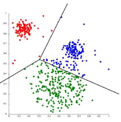
cluster-data. The algorithm figures out which cluster center that it is closest to each data-point and makes them a part of their respective cluster. The next step is to recalculate the cluster center by using the points that are included in the cluster. This process is repeated until the cluster centers are stationary, which gives the correct clustering. As the initial process involves a random starting point for the centres, the method is not deterministic; different runs with the same data can yield different results. However, as the algorithm is quick to process, it is often done multiple times (with different starting values) to get an averaged result. As all points are assigned to the “closest” cluster there are, by definition, no outliers. This means that a single extreme data point can skew the results of a clustering [11]. A graphical representation of an examplek-means result set can bee seen in Figure
2.1.
The k-means clustering is an algorithm that is simple to implement, and that gave
reasonably good results with the right parameters. The main problem with it for our project is that we do not know how many clusters that will be present in our data. Thus, we need to be able to have a cluster algorithm that also can find out how many clusters, if any, it can find.
Determining the number of clusters
Thek-means method does not tell us anything about the number of clusters that are present
in a data-set. It divides the data into the number of clusters given as input. As it is not computationally intensive, we can compute clusters for a range of different numbers of clusters, but that still does not tell us anything about how “good” the clustering is. To do this we can look at how much information we gain for each additional cluster [19]. How good the information is can be measured by looking at the average square distance to the center of the cluster for all data-points. When the second cluster is added the total distance will be significantly smaller. For each added cluster the distance will decrease until we reach the number of unique data-points. The decrease in distance will however pan out and stop the steep curve at a specific point. This will create something called anelbow
[19] which is demonstrated in Figure 2.2. That point can then be used as the appropriate number of clusters, ork.
The elbow is primarily done by hand, which was a problem for our automatized solu-tion. We wanted the system to find out the number of clusters using a formalized algorithm.
Gap Statistic
The Gap statistic is a way of formalizing the elbow process. It evaluates the cluster quality and compares it with the quality of clustering of a uniform data set spread over the same region [19]. The information gain in the original clustered data is compared to the average
Figure 2.1: An example result ofk-means cluster analysis. The
data points have been clustered into three different clusters. [6]
Figure 2.2: Illustration of theelbowof a curve.
information gain of the reference clusterings to decide on which k-value that gives the
2.2 Clustering
For our first implementation we used k-means clustering with Gap-statistic, but the
limitations were too many for it to be a suitable clustering algorithm. Regarding the Gap-statistic as such, we got good results, but due to the number of reference clusterings that were required it was scaling too poorly to be a feasible alternative.
2.2.2
DBSCAN clustering
Density Based Spatial Clustering of Applications with Noise(DBSCAN) is a cluster
algo-rithm that is based on density instead of proximity to the cluster center (like for example
k-means) [8]. It is based around the idea that every node finds its neighbours, the points
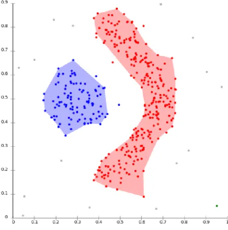
that are within a defined distance away, and if there are enough points they will create a cluster and drag their neighbours into the cluster recursively. If there are not enough of nearby clusters the point will be classified as noise. This also means that the algorithm ac-tually can find clusters of arbitrary shapes and not only circular ones. It also does not need to know how many clusters that are present in the clustering as it finds all of the clusters that fit the criterion. This makes DBSCAN a better choice thank-means for our project.
An example DBSCAN result set can be seen in Figure 2.3.
The DBSCAN still has some parameters that need to be supplied, such as the maximum neighbour distance and number of points that are required to find a cluster. These values depend on the data set that is supplied and what information one expects to get from the clustering.
Figure 2.3: An example result of DBSCAN cluster analysis. The
data points have been divided into two clusters. The grey points are noise. [5]
2.2.3
Fuzzy clustering
The previous mentioned clustering techniques are all examples ofhard clustering. This
means that every data point is selected to be a part of one single cluster, and that cluster only. It is possible for a point to benoise, but it can not at the same time be a part of any
other clustering. Neither it is possible to tellhow muchit is part of the cluster, as a point
in the center and one that is close to the “edge” are equal members of the cluster. This is something that is solved infuzzyclustering. The fuzzy clustering introduces a concept
of membership between the data points and the clusters, allowing the data points to have varying degrees of membership of different clusters. Because of these benefits, we decided to use a fuzzy variant of DBSCAN, the so calledFuzzy Neighborhood DBSCAN.
Fuzzy Neighborhood DBSCAN
Fuzzy Neighborhood DBSCAN (FN-DBSCAN) is a fuzzy clustering algorithm based on
regular DBSCAN. It works almost in the same way as the regular DBSCAN, with the difference that in FN-DBSCAN, a point in a cluster can be either acorepoint or aborder
point. A core point is definitely a part of the cluster, while a border point is only a member of the cluster to a certain degree. A core point is a data point that has a set cardinality that is greater than the minimum cardinality (minCard), which is given as a parameter to
the clustering. The fuzzy set cardinality FSCard(x) of a point is defined in (2.1). It is
calculated as the sum of the so called membership function of a point x and every other point in the data set. The membership function M(x,y) is defined in (2.2), whered(x,y)
is the distance between points xandy, and is given as a parameter to the algorithm. FSCard(x)= n X i=1 M(x,yi) (2.1) M(x,y)= 1−d(x,y)/ ifd(x,y)≤ 0, otherwise (2.2) Each core point will only be a part of a single cluster, and by definition have the maxi-mum membership degree of 1. A point that is not a core point, but is a neighbor to a core point, will be considered a border point of the same cluster that the core point is a part of. Its membership degree will be equal to the membership function of the point and its closest core point neighbor of that cluster. Two points x and y are neighbors ifM(x,y)> 0.
Every point that is not either a core point or a border point will be considered noise.
2.3
The Bank Game
ITSs can be applied in many domains. They are often used for teaching different types of math and other areas that can be described in well-defined models, e.g. the domains of natural sciences and also language [22]. The Bank Game is a set of exercises used
to teach basic arithmetics to children. It is based on the Montessori school of thought, which puts a lot of emphasis on using concrete physical objects in its education, to make abstract concepts easier to understand [15]. The Bank Game was originally created 1917
2.3 The Bank Game
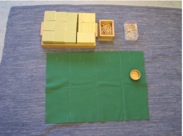
by Maria Montessori, an Italian Physician and educator that was the founder of the still popular educational philosophy called "Montessori". The exercises are built around a set of physical material that uses beads to represent numbers. Figure 2.4 shows a typical Bank Game setup.
There are commonly four different types of objects that each represent a certain numer-ical value. A single bead represents 1, and is called aone-bead. Ten beads held together as
a bar represent 10, and are called aten-bead. One hundred beads configured with ten
ten-beads represents 100 (called ahundred-bead). One thousand beads configured as a cube
with ten hundred-beads stacked on each-other represents 1000 (called athousand-bead).
This means that the size of the objects are proportionate to their value. If two collections have the same size they have the same amount of beads and represent the same number.
The bead material is used in many different exercises. They can be used, in slightly dif-ferent forms, for all of the basic arithmetic operations. One common step in these exercises is that the students need to make an exchange. For example if they add 5 one-beads and 9 one-beads they end up with 14 one-beads, where ten one beads should be exchanged for one ten-bead. This leads to the students constantly having to convert between the different kinds of bead set representations.
2.4
Cognitive aspects
When designing an educational game targeted to children, there are some things that need to be considered. Children are in general very good at learning how to operate different game mechanics and manipulating objects using touch screens [21]. They are, for example, good at learning what buttons to press and where to click on a screen in order to advance in a game. This does not necessarily mean that they have learned the reasons or rationale behind their actions. In these cases they are simply good at “mechanically” operating, without understanding why.
How the interaction with the game is constructed can make a lot of difference in the ability to transfer the skill of playing the game to actual knowledge about math. When children are solving traditional math problems (either by paper or physical objects) the only limiting factors are the numbers and the objects sizes and shapes. And that is often something that is supposed to make the child recognize if an answer is unreasonable. They are still free to answer what they come up with, and can finalize the exercise before getting feedback from a teacher or a correct answer. In a digital learning material it is very easy to give (not necessarily good) feedback, and difficult to grant freedom. The feedback comes from the fact that the users actions is watched at all times and an action can be triggered as something is wrong. This instant feedback means that they get a second chance to do the current step and correct themselves. But this is quite different from the real life where you need to be able to be confident in your solution and solve them without constant help.The problem with lack of freedom origins from the fact that the digital material is software that needs to be developed and created to fill the specific need. Every interaction that is implemented rises the complexity and the time it takes to develop.
As the exercise that is used in this project is complex and contains multiple steps we had to make sure that it was not too easy to proceed in the game without learning the mathematical skill. To achieve this and preserve the pedagogical integrity the teaching material was developed to be as close as possible to the physical exercise. If the interface gives immediate feedback when input is given, it is easy to guess until the right answer is found, i.e. apply a “trial-and-error” strategy. However, if the interface does not directly tell the user when he is right until he has confirmed that the given input is final, the user can not guess and has to reason.
Chapter 3
Approach
In this chapter we will go through the major implementation details of our ITS. Every relevant aspect will be addressed in depth in its respective subchapter, but first it can be useful to get a brief overview. The ITS was implemented as an Android application. A digital version of the Bank Game was created for use as a graphical interface to provide exercises to the users. Model tracing was implemented and used for error detection. The FN-DBSCAN clustering algorithm was used to implement a two-step clustering algorithm for placing the detected errors in groups representing possible misconceptions.
3.1
Development platform
The system was developed as an Android application. This meant we could develop the prototype with touchscreen interaction in mind, and that made it easier to translate the exercise to the digital form. Children generally have a lot of experience with touchscreen devices making them more at home with the platform. On the negative side the Android de-velopment environment set some limitations to what libraries we could use in our project. Java is a widely used language with a lot of AI-libraries, but not all of these libraries, de-pending on language level and performance requirements, are easily used in an Android application.
As Android applications have limited storage space and connectivity and might be used by multiple different people (especially in a school environment) we aimed to make the application ready for utilizing cloud based storage. Saving errors when there is not any connection and uploading them at a later date is something that we had to take into account while designing the solution. This also makes it possible, in the future, to use the device as a gathering device and do all of the computations on a central server (extending the number of possibilities of languages and libraries that can be used).
3.2
Process
The application was developed in an iterative manner, where the different parts were tested and evaluated by real users (both children in the target group and teachers) as a part of the process.
3.3
Digitalizing the physical Bank Game
ex-ercise
A key part of the project was to convert the analog Bank Game exercise into a digital version, that can be understood by a computer, without introducing the game too abstract. A big part of this was to be able to translate the bank exchange action into something that is easily understood, and works on the limited display area available. As the application is targeting a younger audience, it is very important that it is usable and not confusing or too abstract.
3.3.1
Constraints / Eliminating interaction errors
Most of the ITS that have been developed throughout the years (such as the SQL-tutor and the LISP-tutor) were targeted towards university students and consequently quite ad-vanced, but still operating well within defined topics [17]. The target audience for the ITS in this covered work are younger children, typically ages 6-9, and the exercises are based on the math skills of that age group. This comes with a lot of challenges that usually do not need to be considered. One example is that the reading capabilities at that age are varying, which means that textual feedback needs to be limited.As the system is supposed to act as a teacher we needed to know how the teacher and the children work with the Bank Game material today. To gather knowledge about the actual interaction we visited a school and attended a few math classes. Our previous knowledge was all based on instructions for assignments concerning addition and subtraction exer-cises and an interview with a teacher. Seeing the interaction between the student and a teacher gave us access to information that cannot be found in literature. We saw how the teachers gradually introduced more complex steps for the children which gave them more responsibility.
We also managed to identify a few different types of feedback from the teacher when the children did something wrong. Most of them were in some way trying to make the children find the problem by themselves. Asking the children if they were confident in their answer was often enough.
3.3.2
The Exercises
The math application created in this project uses a few different exercises. They are taken from a traditional Montessori material for preschool and first grade students and use thegolden bead materialthat was originally introduced by Maria Montessori in 1917
3.3 Digitalizing the physical Bank Game exercise
3.3.3
Addition
The addition exercise gives the user (child) two numbers that are supposed to be added together. The two numbers are both between 1000 and 9999. The first step for the user is to represent the two numbers with the appropriate configuration of bead representations (one-beads, ten-beads, and so on). The next step is to bring all the bead representations together, i.e. the actual adding. If any of the piles contains ten or more of any of the respective bead representations there there is need for an exchange. (We can not work with, for example, 12 beads, but they need to be converted into 1 ten-bead and 2 one-beads). Finally the user needs to count the beads and answer with the correct number.
Step 1
The user is asked to represent the number 2596 with the appropriate configuration of bead representations on the board. The user then grabs different bead representations from the bank until the board has 2 thousand-beads, 5 hundred-beads, 9 ten-beads, and 6 one-beads. (The user can add and remove beads freely.)
Step 2
The user is asked to add 4367 beads to the board. The user adds 4 thousand-beads, 3 hundred-beads, 6 ten-beads and 7 one-beads. This means that there is a total of 6 thousand-beads, 8 hundred-thousand-beads, 15 ten-thousand-beads, and 13 one-beads. (The user can add and remove beads freely.)
Step 3
The user is asked to summarize the beads, i.e. perform the addition of the two numbers from step 1 and step 2. If there are ten or more bead representations of a specific type the user needs to do an exchange. The user then exchanges 10 of the one-beads with a single ten-bead. Then the user is supposed to exchange 10 ten-beads with a single hundred-bead. This means that there now are 6 thousand-beads, 9 hundred-beads, 6 ten-beads, and 3 one-beads. (The user can only do exchanges with the beads).
Step 4
The user is asked to give an answer. The user counts the bead representations and picks the correct number in a pop-up menu for each type of bead. The user selects “6000”, “900”, “60” and “3”. (The user can only select the number cards)
3.3.4
Subtraction
The subtraction exercise follows the same pattern as the addition, but instead of adding the two piles together the second pile is removed from the first pile. This means that the resulting beads will give the answer. If more bead representations should be removed from a specific pile than the number of existing bead representations the student needs to do an
3.4
System design
The solution proposed in this project has four distinct parts. The graphical interface, the model, the classification module, and the analyzing module. The user interacts with the graphical interface while doing the exercises. Model tracing is used to detect erroneous user actions due to misconceptions. When an erroneous action is detected, the state of the model is saved for further analysis, and when an analysis of the data is started the stacked errors are picked up by the classification module, which performs a set of clusterings that assign every error to a set of classes/clusters. With this information the analyzing module can find which classes that are most prevalent and how the different clusters relate to each other.
3.4.1
Graphical interface
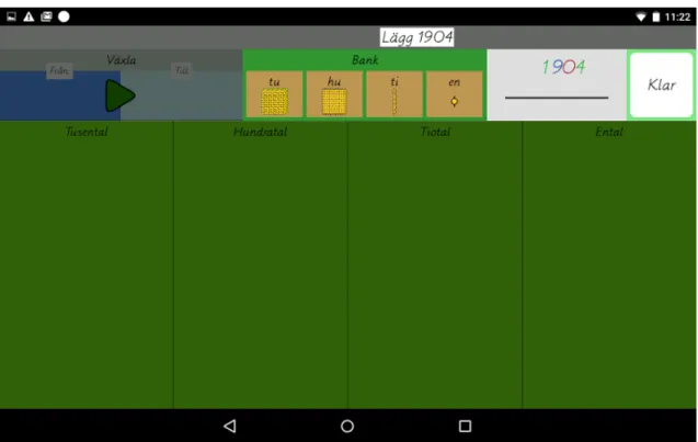
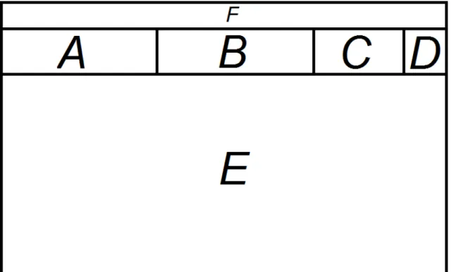
Figure 3.1 shows the graphical user interface (GUI), and Figure 3.2 shows an overview of the GUI (exchange box, bank, assignment paper, finish button, taskbar, and game board).
The bank acts as a source of beads; it is possible to take beads from it as well as to deposit beads in it. The assignment paper shows the current assignment (or exercise) that is to be solved. The game board is the main game area where beads can be placed and moved around. The exercises are step based, and the taskbar shows information about what to do in the current step. The OK button is pressed to proceed to the next step of the exercise.
Walkthrough of an addition exercise
At the start of an exercise, the user is told by the taskbar to place (or represent) a certain number on the game board. This is done by dragging beads from the bank. For example, if the number is 1234, the user must drag one thousand-bead, two hundred-beads, three ten-beads and four one-ten-beads to the game board. As seen in Figure 3.1, there is one column per type of bead. This corresponds to the positional system of numbers. However, the user is free to place beads anywhere on the game board, and is not restricted by the columns in any way. After this, the user presses the OK button and proceeds to the next step.
The next step entails placing the next number on the board. After this, the user once again presses the OK button. At this stage, it is time to add the two numbers, and then make sure that there are less than 10 units of each type of bead representation. This is done by exchanging bead representations with each other using the exchange box. For example, if there are 13 one-beads on the game board, then ten of them should be exchanged for a ten-bead. The exchange box is disabled in all steps except during the exchange step, rendering it impossible to use.
To perform an exchange, the beads that are to be exchanged from are placed in the from-section of the exchange box. Then, the beads that should come in return are dragged
from the bank to the to-part of the exchange box. Next, theperform exchange-button in
the middle of the exchange box is pressed. The beads in the from-part disappears, and
the beads in the to-part automatically gets placed on the game board. The user repeats
3.4 System design
representation corresponds to a position in the positional system, and it is only possible to have nine or less in each position. When done with this step, the OK button is pressed.
After this, it is time to give a numerical answer. The user counts the amount of each bead representation amount, and enters a numerical answer using a pop-up numerical an-swer menu. To be able to provide a correct numerical anan-swer, one must be able to under-stand how the beads represent numbers according to the positional system, which is one of the main pedagogical goals of the Montessori Bank Game.
When the user has entered a numerical answer and pressed the “OK button”, the correct answer will appear, and the user’s answer will be moved next to it so that the user can compare and see if it is correct or not.
Figure 3.1: The graphical interface of the teaching software.
Evolution of the exchange box
The development of the exchange box required a lot of help and we went through several iterations of design ideas, coding, implementation, and user testing. The part that was most challenging was how the exchange mechanism was supposed to work. In the real world, as we had observed in our field studies, the user usually grabbed all of the bead rep-resentations to be exchanged in one hand (whilst carefully counting them), put them all in the bank at the same time, and right after grabbed the appropriate amount of “exchanged” bead representations from the bank. On the virtual game board it is not that easy. As we decided to work in a 2d-world it was a difficult task, both from a visual and interaction point of view, to work with multiple objects at the same time. Single object manipula-tion (such as “drag-and-drop”) is a pattern that is well developed and understood by most people (not the least children [21]). The multi-object functionality is not that obvious,
Figure 3.2: the different parts of the GUI. A is theexchange box,
B is thebank, C is theassignment paper, D is theOK button, E is
thegame boardand F is thetaskbar.
We found many ways to make the exchange easy, but that also proved to be a part of the problem. It was important to keep the difficulty similar to the physical version, in order to maintain the same learning efficiency. Furthermore, the children should learn why they are doing something and not only how. We want them to learn how to solve the exercise (i.e. the pedagogical intention), not how to play the game. The final version of the exchange box has three different parts. A from-box, ato-box and a button to execute
the exchange. This gives the child the task to drag what it wants to put into the exchange box (bead representations from the play field) and specify what it wants to get back (from the bank). When they are satisfied with the exchange situation, they can press the button to confirm their decision. This also means that it is possible to keep track of the exact exchange that the user intended to do.
This design enables us to know exactly what kind of exchange the user makes. In the real world, a person can take bead representations from the exchange box, and also put bead representations in it as many times as he wants, and in any order. If performed that way, it can be hard for a computer to keep track of exactly what was exchanged for what. While it is much easier to “describe” the exchange with the design described above. The drawback is that the interaction of this design differs from the way exchanges are carried out in the real world, and the users might not know directly or intuitively how to do an exchange just from looking at the graphical interface.
3.4 System design
3.4.2
Domain Model
In the beginning we wanted to build a strict ACT-R domain model using jACT-R, but we later decided against this for several reasons. Recall that ACT-R is a very general archi-tecture, with the goal of imitating how the human mind works. The jACT-R model files are specified using a very low-level syntax, to adhere to the ACT-R standard. There are no explicit arithmetic operations available, so everything that is needed has to be created using chunks and production rules. This makes the addition of two numbers very cumber-some to code. First it is necessary to add chunks that contain the relations of the different numbers. For example, one chunk that says that after 1 comes 2, and another that says that after 2 comes 3, etc. At first we implemented our domain model according to this, which resulted in a high amount of duplicated code. The model specifications were also somewhat difficult to read and comprehend, and furthermore, jACT-R is a relatively large dependency, which decreased the performance of the application.
To get around these issues, we decided to implement our own simpler syntax for de-scribing models (inspired by ACT-R but not adhering to the strict philosophy of repre-senting the human mind). We allowed for arithmetic expressions and a much more liberal chunk access. In ACT-R, chunks need to be explicitly loaded into buffers in order to ac-cess their slots. This means that you have to construct your models in a very low-level fashion, as you can only affect a small number of chunks (or facts) at a time. We allowed for direct access of any chunk slot at any time. This way we could get rid of all the abstract production rules, needed in the first ACT-R model, that didn’t correspond to user actions in the real world. With our new system, every production rule corresponds to a concrete user action, like the picking up of a bead representation, or the press of a button, etc.
Our models are defined using JSON syntax and to get a feel of its structure, a simple example model is shown in Listing 3.1. The example defines acounterchunk type, that
has apositionslot with the default value of 0. There are two chunks, and both are of the
counter type. They are calledtarget andcurrent, and the target chunk sets its position slot
to 10. The only production rule is calledincrement-current, which has one precondition
on the left-hand side and one statement on the right-hand side. To fire the production, the position slot of the current chunk must be less than that of the target chunk. When fired, the production rule will increment the position slot of the current chunk by one.
The models are built to reflect what happens on the game board as closely as possible. When a user picks up a bead from the bank, the model fires a production rule to match exactly this. When the user releases the bead somewhere, the model fires another cor-responding rule. The different exercise steps are represented by state slots in the model. What productions that are legal to fire depend on what state the user currently is in.
Listing 3.1: Example of model
{ " model " : { " i d " : " Counter Example " , " d e c l a r a t i v e " : { " chunkTypes " : [ { " name " : " c o u n t e r " ,
{ " name " : " p o s i t i o n " , " v a l u e " : "0" } ] } ] , " chunks " : [ { " name " : " t a r g e t " , " t y p e " : " c o u n t e r " , " s l o t s " : [ { " name " : " p o s i t i o n " , " v a l u e " : "10" } ] } , { " name " : " c u r r e n t " , " t y p e " : " c o u n t e r " , } ] } , " p r o c e d u r a l " : { " p r o d u c t i o n s " : [ { " name " : " increment−c u r r e n t " , " c o n s t r a i n t s " : [ " c u r r e n t −> p o s i t i o n < t a r g e t −> p o s i t i o n " ] , " a c t i o n s " : [ " c u r r e n t −> p o s i t i o n := c u r r e n t−> p o s i t i o n + 1" ] } ] } } }
Connecting to user input
We used an event-based approach to connect the domain model to the user input. Every time the user does something of interest, like picks up a bead representation from the bank or performs an exchange, an input event is created and sent to the model. Every input event is coupled to a production rule in the model. The model checks if the preconditions
3.4 System design
of the production rule are matched and then fires the production. If the preconditions are not met, the production will also fire as we still want the game to continue. If a production rule is erroneously executed, the state of the model will be saved in an error log for further analysis.
Modularity
To add a new type of exercise, one has to create a new model. Depending on the type of exercise, one might also need to make changes to the GUI. The GUI is currently not modular, which makes it hard to extend the system with new exercises. The input events created in the GUI are tightly coupled to the production rules of the existing exercise.
When an error occurs
When the model fails to trace the user’s action, an error has been made. At that point in-formation about the current state of the model is saved for analysis. What is saved depends on the production rule that is broken and it is specified in the model file. The expert model is able to know which rule the user attempts to fire as every user input event is coupled to the firing of a certain production rule. An example of what can be saved could be the number and type of bead representations currently on the board, or the correct numerical answer for the specific exercise.
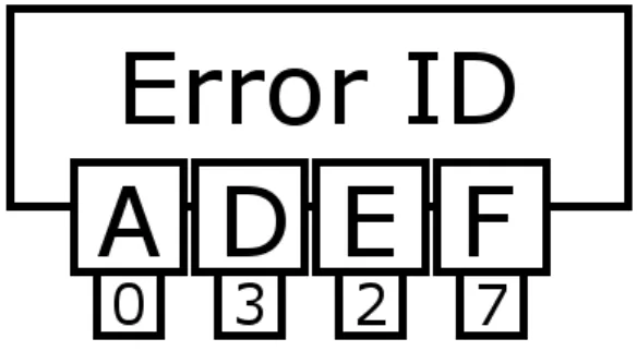
Figure 3.3 shows a symbolic view of a saved error. The production rule that was er-roneously fired (and thus caused the error) decides which features to save. These features are represented by A, D, E and F in the figure. Which features to save are defined for each production rule in the model. The values of the features below the letters in the figure represent the values of the features. Each error is assigned a unique ID.
Figure 3.3: A schematic view over a saved user error. The error
saves the values (here 0, 3, 2 or 7) for the different features (in this case A, D, E and F) that are defined in the model corresponding to the current state.
Multiple errors
As an error occurs when the model cannot track the user anymore, everything done by the user after an initial erroneous action is by definition also an error. Taking care of these more complex chains of errors was out of scope for this thesis, so only the first error of each game is saved. One way to tackle this issue could be to, after logging the error, consider
the erroneous action from the user as a correct one and then continue on with the game. If the user does something wrong, it is still interesting to see if he acts correctly during the remainder of the exercise.
3.4.3
Classification module
The errors that are detected are saved to the internal storage of the Android device for future analysis. When the user initiates the analytic phase all of the collected errors are first classified, to be able to know how they relate to each other. The point of this is to group them together based on possible underlying logical structures, or misconceptions.
Making errors comparable
To be able to find which errors that belong to the same misconception there needed to be some kind of comparison between them. Our first approach was therefore to cluster them. To be able to do that we needed to compute thedistancebetween two errors. A strength
of clustering is that it can be applied to multiple dimensions, putting a separate feature in every dimension, which gives the possibility to compare a lot of different features. In our case, it facilitated the input of numerical information such as the number of beads on each side of an exchange. However, other kinds of information can be harder to put into comparable numerical values, such as the current state of the exercise.
Features
There are a number of different errors that the user can make in the application. For example having the incorrect amount of beads in the left or right exchange box, or putting the wrong number of beads on the game board. Every error produced by the user has a specific set of features. Some features exist in all errors, such as what the correct outcome of the exercise was, while other features are only present in some errors. Which features that are saved for a specific error are decided by the chunk that the player currently is in, and is configurable in the model file (cf. Listing 3.1).
The reason for not always saving the same features for all errors is that all parts of the game are not always active, like the exchange box for example. As it is disabled until the exchange step is reached, this should not be considered when saving errors in other steps. Likewise, the content in the exchange box is not relevant when at the first step, in which the user is supposed to place a number on the game board. Information about the current step together with the chunk information is saved to local storage.
Grouping features
A single clustering instance is defined by a number of features needed for an error to be considered in the instance. The system gathers all the errors that contain all of the included features and clusters them, labeling the error with a specific class, or cluster id, for that specific feature-set. Consequently, an error will not be present in all clusterings, but only in the ones that it actually can contribute to. The result will be a number of different feature-sets with a number of errors each (i.e. clusters).
3.4 System design
Choosing a clustering algorithm
The first implementation of the classification module used the k-means clustering
algo-rithm (see Section 2.2.1). It is a simple algoalgo-rithm and the only challenge was to find out how many clusters that were actually present in the data (thek-value). This meant that the
clustering would have to be done for several different values ofk, so that the best fitting
clustering could be selected.
We first tried to do a simple implementation of the elbow method by looking at the derivative of the error distance for the differentk-values. The results were not too
con-vincing and we decided that there was a need for a better approach. Instead we went for the Gap statistic (see Section 2.2.1) to get a better and more formalized version of the elbow method. The Gap statistic gave us more reasonablek-values, but was a lot slower
than our first implementation. The reason for this was that eachk-value that was
investi-gated required a number of uniform reference clusterings computed before the algorithm converged. As we had several different clusterings to do, one for each feature, the scala-bility for this approach was very bad. Another problem was that because of thek-means
indeterministic nature we got some inconsistent results on consecutive runs.
This made us try a different clustering algorithm, the DBSCAN-algorithm. It only required a single clustering computation, could figure out the number of clusters without running additional computations (compare with the Gap statistic of thek-means algorithm)
and showed an overall better run time performance for our specific use case. First we used the regular DBSCAN algorithm, but then changed to the fuzzy variant FN-DBSCAN instead to enable for errors to have different degrees of cluster membership (See Section 2.2.3).
Making clustering work
Our first approach to clustering was to put all the information about each error-state into an multi-dimensional vector and try to get information out of it. The basic tests that we ran showed that it was hard to get valuable data out of the clustering due to large differences in a few variables would be enough to counteract the potential proximity in the others. Furthermore, it is known that the effectiveness of clustering diminishes with the number of dimensions used, which is commonly referenced to as thecurse of dimensionality[12].
To get around this problem we decided to divide the features of the error into specific feature-groups and cluster each feature-group on its own. This was done by creating a number of predefined cluster instances. With this we could classify the features with a higher precision and each error would be classified into a number of clusters. The inter-esting part is what can be extracted from this information. One can for example look at the size of the different clusters and check if one cluster contains significantly more errors than others. It is also possible to compare errors classified into the same clusters.
Clustering instances
The clustering algorithm is run several times using different features. Each such instantia-tion is hereafter referred to as acluster instance. The clustering is done by several different
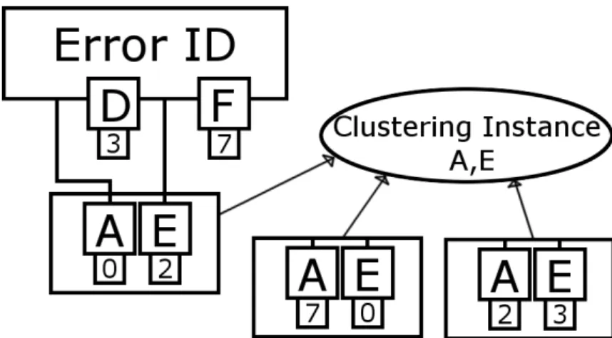
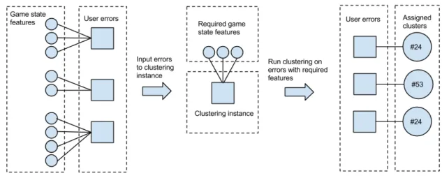
to the full list of errors and can extract all of the features (such as the number of thousand-beads on the game-board or the number of one-thousand-beads in the right exchange box) that it needs to do its clustering. If an error is missing any of the features that a specific instance needs for the clustering it is omitted from that instance. The instances can also preprocess the data if they need to cluster on something that is not directly stated in the error (such as the total number of beads in an exchange box) or if the data needed to be normalized. When the clustering is done, every error (or data point) is assigned a cluster, which can also be referred to as its “class” of the error. This means that during the clustering process each error will gain a list of the different classes that it is part of, one for each clustering instance that is applicable. The instances make it easy to add, remove and modify what features the system uses for clustering. An overview of the clustering instance system can be seen in Figure 3.4.
Figure 3.4: Each instance goes through all of the saved errors and
picks out the ones that have the relevant features. For every such error it selects the needed features and generates a data point in the clustering for it.
What instances should be used?
The distributed clustering system (in contrast to cluster on everything) means that we have to take an active role in deciding what the system should cluster on. Preferably this is something that, in the future, can be evaluated using a machine learning algorithm to find which features that actually belong together. For this project we did not have any data to base or train the system on, and thus we relied on a couple of educated guesses. Some of the things that we decided to cluster on was:
• Current board content (number of one, ten, hundred, and thousand-beads on the game board).
• Current exchange box content (number of one, ten, hundred, and thousand beads in both of the exchange boxes before an exchange).
• Answer to the current exercise.
3.4 System design
3.4.4
Analytics module
To analyze the errors, several different approaches were tried. Here we briefly discuss our initial approaches, and then go through the final approach in more detail.
Initial approach
Our first approach to get some information out of the clustering was to look at similarities between different errors, i.e. if they had been assigned the same clusters. How similarly two different errors have been classified could possibly give some information about their cause. If they are very similar it might indicate that the cause of the errors is related to the approximate feature values of the clusters that the errors have in common.
Another approach was to use a Bayesian network, where every clustering was a node and every cluster was a specific value of that node. However the only data that we could train on was data that we had created ourselves (as we cannot tell for sure what miscon-ceptions a real person might have), and that means that we could only detect the specific misconceptions that we decided to train it on. A big challenge was that we had no real world training data describing the actual misconceptions.
Final approach
After some consideration we turned to another solution. We decided to make a second clustering, using the output of the first clustering step as input (See Figure 3.7. Here the clustering was done on the classes (clusters) that they belonged to. The distance be-tween the different data points was now dependent on how large percentage of clusters they shared. As the DBSCAN algorithm had proven to be effective we decided to try it again. A threshold was set up for how large percentage the data points needed to share to be considered to be neighbours.
Fuzzy clustering
After some testing with the standard DBSCAN algorithm, we decided to also evaluate a fuzzy clustering approach, so we switched to FN-DBSCAN. Our idea was that thedegree of membershipwould give us more info in the classification module, which then could be
used in the analytics module to make it easier to find patterns.
To do that we needed a new way to measure thedistance(See Section 2.2.3) between
the different classified data points. Each data point would now have a two-dimensional array of class membership, i.e. for each clustering instance it would belong to multiple classes with varying degrees of membership. To measure the distance we decided to com-pare each clustering instance separately, and for each cluster in that instance we would sum up the differences indistanceeach of the instances. This means that if both data points
have a membership of 0.6 of cluster A they would be considered identical. If one have a membership of 1 and the other 0 they would be regarded as being the maximum distance away from each other.
The score for each cluster is averaged and added up with the score from the other instances which gives a value that can be seen as a distance. It is important to note that
together. The most obvious example of this is when the membership is 0 for both data points, which only tells us that they are not related to that point in any way. The point of this measurement, however, is to group points that have a similar membership profile. If two points are very similar in their relation to all of the clusters in an instance, they
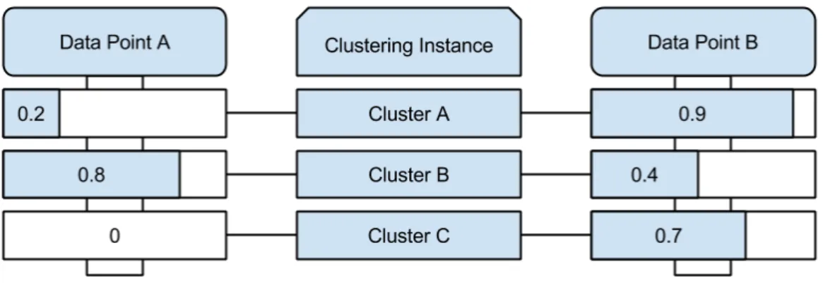
follow the same pattern and should therefore be considered to be close to each other. This is illustrated in Figures 3.5 and 3.6.
Figure 3.5: Example of comparing two data points. The two
points are not identical, but have similar membership to the dif-ferent clusters. Therefore the points will have a short distance be-tween them (i.e. they will be “close” to each other).
Figure 3.6: Another example comparing two data points. Here
there are big differences in the membership values which leads to the points having a long distance between them.
Determining parameters
Even FN-DBSCAN has its set of parameters that have to be provided for it to be able to do a good clustering. The minimum cardinality (See Section 2.2.3) to determine core points and the maximum neighbour distance are some of the things that need to be provided for the algorithm to work. These values can be estimated based on different properties such as the number of data points and the min/max value, but there is no correct answer. No set of parameters will ever give a false result — they will just show the clustering from a specific
3.5 Combining the modules
perspective, although some are more useful for extracting information than others. The challenge is to find a perspective that gives us the information we are searching for, as we want to see if our approach could be viable. No formal method to determine the values of the parameters was available, so we had to do some educated guesses (See Section 4.3.2 for the chosen values).
3.5
Combining the modules
When the errors are analyzed, the modules work together as seen in Figures 3.7 and 3.8. First, the user errors are retrieved from storage. Then, for each clustering instance, the errors that have the required saved features (which depend on the production rule that was broken at the time of the error) are clustered and assigned a cluster. This is done once for each clustering instance. Then it is time for the second clustering pass, as seen in Figure 3.8. Here all the user errors are clustered based on what clusters they were assigned in the first clustering step. This will create clusters of user errors, that relate to possible misconceptions which might have caused the errors. Note that each can be assigned to several clusters in the classification step; one for every clustering instance at the most.
Figure 3.7: The classification step. This is done once for every
Figure 3.8: The analytic step. This is done once after the
Chapter 4
Evaluation
In this chapter we go through the results found when running the system in various ways.
4.1
User test
To get an indication of the usability of the digital Bank Game application and collect some error-data for testing purposes we conducted a user test at a Montessori school in Hjärup, Sweden. The test was conducted on a set of students with varying experience of the bead materials. The interaction worked fine, with the only exception being the exchange step. This was somewhat expected, as described in theEvolution of the exchange boxsection in
Chapter 4 (Approach). It did not lead to any further changes in the interface, as the ease
of use of the system was deemed acceptable. The error data collected gave us some kind of insight to what the system might receive in the future.
The user interaction part of the application has been evaluated continuously throughout the project by a set of small and quick user tests. The feedback has been used to improve and completely rework certain parts of the system.
4.2
Testing with DBSCAN and simulated
mis-conceptions
To test the system, we wanted a user with a known misconception to play the game, so that we could try to find the misconception after looking at the errors made. As it is hard to know exactly what misconceptions a human has, we decided to create a computer player for the game. This computer player plays directly into the model and thus circumvents the graphical interactive user interface of the game. The computer player plays according to pre-scripted strategies/rules which means that we can introduce known misunderstandings
into the student model. The data collected therefore has a known cause that we could try to recover using our implemented DBSCAN model, and thereby evaluate our solution.
The simulated player does three different kinds of mistakes:
• It sometimes exchanges five ones for one ten-bead, and five ten-beads for one hundred-bead etc.
• It sometimes exchanges ten ones for ten ten-beads, etc.
• It sometimes presses the ready-button without putting the correct amount of beads on the game-board.
These are all artificial misconceptions, that do not necessarily exist in the real world. We assume that they do not have to be realistic, as we are not so much interested in the mis-conceptions themselves, as we are in valuating our model by finding similarities between their resulting errors.
4.2.1
Clustering misconceptions
The second clustering of the data points, using the classes as distance, gave some interest-ing results when usinterest-ing errors from the computer player. For this specific error the player was programmed to do two different mix-ups in the exchanges, sometimes it would: (i) exchange 10 one-beads for 10 ten-beads, instead of 1 ten-bead, etc, and (ii) exchange 1 ten-bead for 5 one-beads (instead of 10 one-beads).
Table 4.1: Statistics for the first test of 20 game sessions
Number of game sessions: 20 Collected errors: 107 Number of misconceptions: 1
4.2.2
After 20 games
Table 4.1 shows how many errors were found after running 20 game sessions with the com-puter player, and that one possible misconception was found. Table 4.2 shows the different clusters after the classification step (first clustering step), with the different feature classes of the data points listed. For example, “num(left exch) vs. num(right exch)” represent the points that belong to cluster #0 of that specific feature. The different classes are structured as follows:
• num(left exch) vs. num(right exch)contains two values, the amount of bead types in
the two exchange boxes. For example, if there are 10 ten-beads in the left exchange box and one hundred-bead in the right, this feature will be [10,1].
• Board content has four values: the amount of beads of the different bead types that
are located on the game board. If there is one thousand-bead on the board and nothing else, this feature will be [1,0,0,0].