VOLUME XX, 2017 1 Digital Object Identifier 10.1109/ACCESS.2017.Doi Number
Improving Load Forecasting Process for a
Power Distribution Network Using Hybrid AI
and Deep Learning Algorithms
Sibonelo Motepe1, Ali N. Hasan1, Member, IEEE, and Riaan Stopforth2, Senior Member,
IEEE
1Faculty of Engineering and the Built Environment, University of Johannesburg, Johannesburg 2092, South Africa
2Stopforth Mechatronics Robotics Research Lab, School of Engineering, University of Kwa-Zulu Natal, Durban 4041, South Africa
Corresponding author: Sibonelo Motepe (e-mail: [email protected]).
The authors would like to thank the South African Weather Services for providing them with weather data. The authors also acknowledge the National Research Foundation, the Eskom TESP programme, and the DST ROSSA programme for partially funding this research.
ABSTRACT Load forecasting is useful for various applications including maintenance planning. The study of load forecasting using recent state-of-the-art hybrid artificial intelligence (AI) and deep learning (DL) techniques is limited in South Africa (SA) and South African power distribution networks. This paper proposes a novel hybrid AI and DL South African distribution network load forecasting system. The system comprises of modules that handle the collection of the loading data from the field, analysis of data integrity using fuzzy logic, data preprocessing, consolidation of the loading and the temperature data, and load forecasting. The load forecasting results are then used to inform maintenance planning. The load forecasting is conducted using a hybrid AI/DL load forecasting module. A novel comparative study of recent state of the art AI techniques is also presented to determine the best technique to deploy in this module when forecasting South African power redistributing customers’ loads. The impact of the inclusion of weather parameters and loading data clean up on the load forecasting performance of a hybrid AI technique, optimally pruned extreme learning machines (OP-ELM), and a deep learning technique, long short-term memory (LSTM), is also investigated. These techniques are compared with each other and also with a commonly used powerful hybrid AI technique, adaptive neuro-fuzzy inference system (ANFIS). LSTM was found to achieve higher load forecasting accuracies than ANFIS and OP-ELM in forecasting the two distribution customers’ loads in this study. Only LSTM models’ performance improved with the inclusion of temperature in their development.
INDEX TERMS Adaptive Neuro-Fuzzy Inference Systems, Artificial Intelligence, Deep Learning, Distribution Networks, Extreme Learning Machines, Load Forecasting, Recurrent Neural Networks, Long Short-Term Memory
I. INTRODUCTION
Electricity has been regarded as South Africa’s gross domestic product’s (GDP) main driver [1], [2]. Developing countries still experience a lack of electricity access [3]-[6]. These countries, including South Africa, have electrification programs that are driving the connection of its citizens to the power grid. South Africa (S.A.) obtained its democracy in 1994, and has since then electrified more than 5.2 million homes and over 12 000 schools [7]. The South African government plans to achieve universal supply by 2025/2026 [8]. In order to achieve this goal, while ensuring continuity of supply, utilities need planning
at different levels of the power system. Load forecasting whose importance was established in different studies including [9] and [10], becomes important in order to achieve a sustainable power supply.
Load forecasting has different windows which it can be classified into. These windows are short term, medium term and long term, which respectively cover hours to weekly forecasts, monthly to quarterly forecasts and then yearly forecasts [11]. With the movement towards the smart grid in developed countries, recent load forecasting studies have moved past the customer supply point [12]-[14]. Appliance power consumption data have been incorporated to forecast
VOLUME XX, 2017 1 load using a fuzzy logic approach [13]. Australian
residential load was forecasted using long short-term memory recurrent neural networks (LSTM-RNN) models developed using smart meter data [14]. Other researchers have moved towards understanding and predicting customer behavior in demand response [15]-[18]. This behavior influences the customer’s consumption/load profile and thus load forecasting [16], [17]. In [15] the nearest neighbor algorithm and Markov chain algorithm was used to predict user behavior and energy management. Recent load forecasting studies are moving towards deep learning techniques [19]-[22]. The rise in the use of these techniques can be associated with the rise in computational power and access to labeled data [23]. These techniques have achieved excellent performance in computer vision, speech and language processing [23]-[27]. The three popular deep learning techniques are convolutional neural networks (CNN), deep belief networks (DBN) and recurrent neural networks (RNN). In [19] cycle-based LSTM and time dependency CNN was used for load forecasting. LSTM-RNN has been shown to be a robust method in load forecasting [28]. LSTM’s performance was found to match that of state-of-the-art techniques and supersedes a few cases [28]. In [20] and [29] the authors found that LSTM-based models performed better than convolutional networks in energy consumption forecasting and natural language processing, respectively. Weather conditions have been included as input parameters in a number of load forecasting studies [10], [30], [31]. These weather parameters’ data are not always collected or kept by power utilities. This data can also come at a cost when sourced externally from the utility and commercially used. Hence, the need to understand if weather parameters improve the load forecasting performance of AI models.
The study of the application of AI in S.A. load forecasting is limited [9], [32]-[38]. Some of these studies are outdated and do not use recently developed techniques [34], [35]. Ijumba’s study is from 1999 and used artificial neural networks (ANN) [34]. Medium-term load forecasting has been seen to be complex and requires more sophisticated techniques such as deep learning over shallow ANN [19]. Despite this recommendation, a recent SA load forecasting study from 2018 utilized ANN [39]. Despite being around for some time ANFIS is still a powerful technique and was the most common technique used in these studies. ANFIS has been shown to be superior to most popular statistical and artificial intelligence techniques [9] [40]. ANFIS is thus used in this study as a comparison base for the performance of the techniques used in this study. Marwalaet al. introduced the recent state of the art extreme learning machines (ELM) and its improved version, optimally pruned extreme learning machine (OP-ELM) in SA load forecasting [32], [33]. Their studies focused on the country’s total consumption and not on distribution level power networks. They also did not compare these
techniques to any state-of-the-art deep learning technique. Yuill et al.’s study focused on short-term load forecasting, with 30 minutes ahead load forecasting using ANFIS [35]. This study was conducted for optimal generation scheduling in SA. Short term load forecasting cannot be used to plan maintenance in distribution networks. The part of the power system value chain that the study data were collected from, was not clarified. This study incorporated weather parameters, temperature and humidity. Their impact was studied for ANFIS only and on a single data set. The impact of not using these weather parameters was not investigated. Motepe et al. found that ANFIS models can achieve better performance in forecasting a SA distribution network’s load without the inclusion of temperature in the model development [37]. This study focused on one AI technique, ANFIS, and load type, a power redistributor. In another recent study, Motepe et al. found that for the same load profile in [37] DBN models achieved better performance with temperature used in the model development [38]. It is thus evident that published research on load forecasting using deep learning techniques in South Africa (S.A.) is almost non-existent. The impact of temperature on the performance of AI and deep learning techniques in SA load forecasting has not been well investigated. Therefore, further studies with other state of the art AI techniques and DL techniques still need to be explored. The impact of temperature inclusion on the performance of these techniques also needs to be investigated further.
This paper contributes to the body of knowledge of load forecasting studies in South Africa through the following contributions: (i) A novel investigation of arecent state-of-the-art hybrid AI technique, OP-ELM, and deep learning techniques in South African Distribution networks load forecasting through two case studies of real SA power redistributors. (ii) An introduction of a novel hybrid AI and deep learning distribution load forecasting system for power redistributor loads. (iii) An investigation of load forecasting performance impact due to temperature inclusion in the hybrid AI and DL models development. (iv) A novel investigation of the load forecasting performance impact due to cleaning up loading data to remove spikes and dips before developing hybrid AI and deep learning models.
The paper is arranged as follow: Section II presents an overview of five AI techniques: fuzzy logic, neural networks, adaptive neuro-fuzzy inference systems, optimally pruned extreme learning machines and long short-term memory recurrent neural networks. Section III presents the proposed hybrid AI and DL load forecasting system. Section IV presents the system and experimental setup. The results are given in Section V. The paper is then concluded in Section VI.
VOLUME XX, 2017 1
II. ARTIFICIAL INTELLIGENCE AND DEEP LEARNING TECHNIQUES
A. FUZZY LOGIC
Fuzzy logic is an expert system that was developed in 1930 by Jan Łukasiewicz [41]. Fuzzy logic has been applied widely in power systems related studies. Motepe et al. used fuzzy logic to determine power consumption data accuracy [42]. In [43] short-term load forecasting was conducted using fuzzy logic. Active power loss forecasting has also been conducted using fuzzy logic [44]. Fuzzy logic systems have a short-fall in that they depend on expert experience to develop the fuzzy rules they operate from. Different experts can therefore build models that give different results from the same data [45]. Fuzzy logic also lacks the ability to learn and to self-adjust to a new environment [10]. The Mamdani inference system and Sugeno/Takagi-Sugeno (TS) inference system are the popular fuzzy logic inference systems. The Mamdani inference system is applied in four key steps: fuzzification of the input variables, evaluation of the rules, aggregation of the rule output and then defuzzification [41]. The main difference between the TS and Mamdani is in the last two steps. The TS type output is either a linear function or constant. Equation (1) defines a TS type output. The TS fuzzy logic inference system is commonly applied in data-driven modeling.
Ri: if z is Ai then yi= ai Tz + ci (1)
where Ri is the rule, Ai is the antecedent, aithe consequent parameter vector, cithebias, i=1,2,….n, y is the output and is given by (2).
=∑ α( )
∑ α( ) (2)
where αiis the ith rule’s degree of fulfillment. The TS model can be considered as a piece-wise smooth linear approximation of the non-linear function. This is due to the TS model parameters being local linear models of the non-linear system under consideration.
B. ARTIFICIAL NEURAL NETWORKS
Artificial neural networks (ANN), also just termed neural networks, are non-linear mathematical processing networks designed to mimic the human brain [46]. Neural networks have been applied in numerous fields, such as load forecasting, image recognition, speech recognition, data retrieval, energy consumption prediction, mine dam water level monitoring and prediction [40], [47], [48]. Neural networks have synaptic weights which connect their neurons. These neurons can have a single output and multiple inputs. The output is derived from the input by the sum of weighted values and the bias as shown in (3) [49].
= ∑ + (3)
where z is the input, y is the output, w the weight and b the bias. The aim of the training is to achieve a minimum error between the target value and the model output. This training is conducted through multiple iterations to fine-tuning the synaptic weights. These iterations continue until an acceptable error is or a set threshold is reached. Equation (4) gives the error function:
( ) = ∑ , − (4)
here E is the total error, y is the model output and t is the target value. The synaptic weights are updated using (5):
+1= −λ∇ ( ) (5)
where s is the iteration step, m is the weights index, λ is the learning rate and ∇E(w), the gradient, is given by (6):
∇ ( ) = "#$ #%&, #$ #% , … … , #$ #%() (6)
The goal is to get a weight vector where E has its smallest value.
C. ADAPTIVE NEURO-FUZZY INFERENCE SYSTEMS
Adaptive neuro-fuzzy inference systems (ANFIS) combine neural networks and fuzzy-logic to take advantage of the two techniques’ strengths and to overcome their shortfalls. Neural networks have shortfalls such as lack of knowledge representability and explainability. Fuzzy logic is not able to learn from data [41]. ANFIS has been used broadly in various aspects of power systems. ANFIS applications include load forecasting, photovoltaics (PV) model optimization for DC-DC converter systems and PV plants maximum power point tracking [9], [50], [51]. The most common neuro-fuzzy model is the Takagi-Sugeno type [52]. Neuro-fuzzy models are seen to be adaptive due to their ability to learn.
FIGURE. 1. The ANFIS model basic structure
∏ ∏ ∏ ∏ a21z1+a22z2+c2 ∑ N N a11z1+a12z2+c1 z2 z1 α2 α1 γ2 γ1 y
2 VOLUME XX, 2017 Owing to this ability to learn, ANFIS models can therefore
be trained using gradient descent as opposed to being trained using expert knowledge. The basic ANFIS structure is shown in Fig. 1. The first layer has adaptive nodes, which compute the input membership degree in the antecedent Gaussian fuzzy sets. The second layer sees the application of the fuzzy AND operator. The normalization (N) and summation (∑) achieve the fuzzy mean operator. The most commonly used form of the Gaussian membership function is given in (7) [52].
*+ , , , - = ./0 1−( 234)5
645 7(7) where δ is the variance of the Gaussian membership function and g is the center of the Gaussian function. The TS relationship between its input and output is given by (8): = ∑ 8 ( ) (9: + ; ) (8)
with
8 ( ) = ∏@4 =>? (2( 234)5( )/δ54)
∑B ∏@4 =>? (2( 234)5( )/ δ54) (9)
The hybrid learning process uses the least square estimator as well as the gradient descent methods. This process involves two key steps:
Step 1: Find the optimal number of rules.
Step 2: Partition the input space to be equally divided with the functions’ width and slopes to allow sufficient overlaps.
The training has a forward and backward pass. The forward pass involves the determination of the rule consequent parameters from the neuron outputs which are calculated using the input data. The backward pass involves the application of backward-propagation, where the antecedent parameters are then updated using the back propagated error signals.
D. OPTIMALLY PRUNED EXTREME LEARNING
MACHINES
With data sizes increasing, big data have become a buzzword [53]. In [53] the authors give definitions of big data. It has been observed that when the quantity of data used increases the computational complexity increases [54]. High computational power is not always accessible. There is, therefore, an inclination for non-linear models not to be used as broadly as they could due to their being slow to build feed-forward neural networks. This reduced usage is despite the feedforward models’ overall good performance [54]. In [55], the authors introduced an algorithm called extreme learning machine (ELM), which reduces the required training computational time and model structure selection of neural networks. The technique is a single layer neural network that was proposed in the mid-2000s by Huang et al. These researchers also demonstrated that this method could be utilized successfully in a variety of applications [55]. ELM
has been used in many other applications by different researchers [32], [56], [57]. In [57] ELM was shown to perform better than traditional artificial neural networks (ANN), radial basis function neural networks (RBFNN) and back-propagation neural networks (BPNN) in most testing datasets, in market clearance price forecasting. The authors in [58] showed that optimally pruned extreme learning machines (OP-ELM) outperform the popular machine learning techniques (ANN, ANFIS and support vector machines (SVM)) and time series techniques (autoregressive moving average (ARMA)). OP-ELM was found to also outperform the standard ELM. To describe the ELM training process, suppose a training set xi is given, where i=1,…..n, with a target vector ti. The ELM’s goal is to decrease the training error function E to be as low as possible. Equation (10) represents the ELM for these conditions:
∑ CE , , / D = (10) where wj is the input weight vector that connects the jth hidden neuron and the input, βj is the output weight that connects the jth hidden neuron and the output and the jth hidden node’s bias is represented by bj. If the ELM model
can estimate the data sample with zero error, that is ∑ ‖ − ‖ = 0, a wj, bj and βj exist so that
∑ CE , , / D = , i=1,….n. Equation (10) can thus be re-written as (11):
HD = I (11)
where H is the hidden layer output matrix and can be written as (12). H = JC( , , / ) ⋯ C(⋮ ⋯ E,⋮E, / ) C( , , / ) … C( E, E, / ) M ×E (12) The input weight and hidden bias have been shown not to require tuning [57]. Therefore, after assigning random values to the matrix H parameters at the start of the training, the matrix can be left unchanged. If the matrix H is square, that is k=n, it is possible to randomly assign the hidden nodes, and the output weights can then be computed through the inversion of H. Hence, the ELM can estimate the data sample with an error of zero. H is in most cases not a square matrix and is thus invertible. A wj, bjand βj so that HD = I may therefore not exist. The ELM training process here corresponds to solving a least square problem. The ELM weight between the output and hidden layer, unlike in conventional neural networks (NN), can be determined through the hidden layer output matrices’ generalized inversion. This operation is known as the Moore-Penrose. The weights can, therefore, be given by (13):
D = H∗I = (HH:)2 HI: (13)
where H*is matrix H‘s Moore-Penrose generalized inverse [32]. The ELM algorithm can be summarized as follows:
2 VOLUME XX, 2017 Step 1: Assign input weights and bias, wj and bj, j=1… k
at random.
Step 2: Determine H, the output matrix of the hidden layer.
Step 3: Determine β, the output weight using (13) The standard ELM has a drawback in approximating underlying dynamics when correlated or irrelevant variables are included in the training data set. The authors in [54] proposed an OP-ELM to overcome these shortcomings. In this approach, the irrelevant variables are pruned by marginalizing the irrelevant neurons of the network built using the ELM. The OP-ELM three key learning steps are as follows:
Step 1: Use the ELM technique to construct the multi-layer perceptron (MLP) model
Step 2: Use multi-response sparse regression (MRSR) to rank the neurons
Step 3: Select an optimal number of neurons using the leave-one-out (LOO) validation method
E. LONG SHORT-TERM MEMORY RECURRENT
NEURAL NETWORKS-
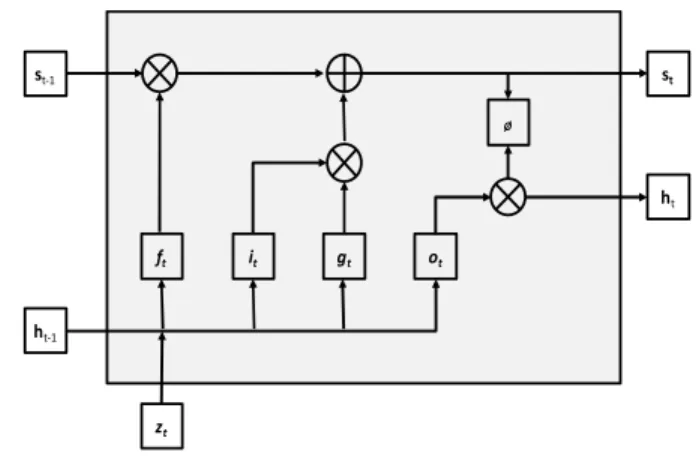
Recurrent neural networks (RNN) with long short-term memory (LSTM) are highly rated as a trustworthy technique in sequential data series modeling, forecasting and analysis [59]. LSTMs are usually used in solving problems in sequential data-related applications such as audio and language. LSTMs are effective in capturing long-term temporal dependencies without facing the optimization challenges faced by the simple recurrent network [28]. LSTM architecture’s key is a memory cell that retains its memory over time. Non-linear gating units regulate the flow of information in the cell. The gating mechanism enables LSTM to succeed in dealing with the vanishing gradient challenge experienced by the standard RNN. The structure of an LSTM unit block, is given in Fig. 2. shows these non-linear gates. When these LSTM units are stacked, the deep LSTM-RNN is attained.
Take {z1, z2,.., zt} as an input sequence for an LSTM, with zt representing a kth dimension real values array at time step t. The memory cell state st-1 and intermediate state ht-1 interact with ztand the previous time step outputs to determine which of the internal state vectors’ elements to update, erase or maintain [14].
FIGURE 2. LSTM unit block structure
The LSTM defines the forget gate (ft), input gate (ii), input node (gt) and output gate (ot) using (14) to (17), respectively. Equation (18) and (19) give the memory cell state and the state at time step t, respectively.
CP= Q(RS P+ RSTℎP2 + S) (14) VP= Q(R P+ RTℎP2 + ) (15) ,P= ∅(R3 P+ R3TℎP2 + 3) (16) XP= Q(RY P+ RYTℎP2 + Y) (17) P= ,P⨀ VP+ P2 ⨀ CP (18) ℎ = ∅( )⨀ X (19)
where Wfz,Wfh,Wiz,Wih, Wgz,Wgh, Wozand Wohare weight matrices for the network activation functions’ corresponding inputs. The functions σ and ø, respectively represent the sigmoid function and the tanh function. The element-wise multiplication is represented by ⨀.
st ht st-1 ht-1 zt ft it gt ot Ø
2 VOLUME XX, 2017
FIGURE 3. Proposed hybrid AI/DL load forecasting system
III. PROPOSED LOAD FORECASTING SYSTEM
The proposed system involves the collection of power consumption data from the field equipment using power meters. These data are then transmitted to a central database for storage and utilization by the utility in different applications. The system overview is given in Fig. 3. The data integrity is determined through a module that deploys fuzzy logic. If the data have low integrity they raise flags to trigger investigations into the causes of the integrity challenges. Once investigated the database and/or field repairs are conducted. The data with high integrity are then pre-processed. This involves the normalization of the data. The temperature data are requested from the weather service and stored in a database. These data are also preprocessed. The model input variables are then consolidated for input into the hybrid AI/DL module. The hybrid AI /DL module is used to forecast the distribution load. The hybrid AI/DL module should have models that have been trained and tested offline deployed in it. The load forecast results are then used to inform the distribution network maintenance plans. The
load forecasting results for different networks are also stored in a central database, for access by different departments in the utility.
IV. SYSTEM AND EXPERIMENT SETUP
Two distribution substations that supply power redistributors are used as case studies in this research. This section presents these two substations as well as their power consumption/loading data. The experiment setup is also presented.
A. SYSTEM SETUP
The two substations used were separated into two case studies, Case Study A and Case Study B. The substations, the overview of the distribution network the substations are located in and the loading data are presented per Case Study in this subsection.
1) CASE STUDY A SUBSTATION AND DISTRIBUTION
NETWORK OVERVIEW
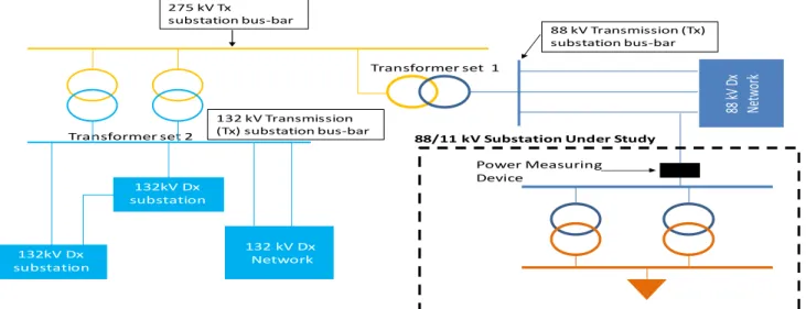
The loading data used in this Case Study were for a distribution substation that was commissioned in the year 2012. These data were collected for a period between August 2012 to May 2016. With the combination of data integrity and the electrification programs, the limited number of years a substation’s data are available for, can be a common case in most substations. These loading data were obtained from a real South African power utility database. These data were logged from a medium voltage distribution substation, measured at the incoming feeder. The substation is connected to the grid through a 275 kV main transmission substation (MTS). This connection is at T-off of an 88 kV feeder from the MTS as shown in Fig. 4. The distribution network shown in Fig. 4. is a 3-phase system. The substation under study has two 88/11 kV, 40 MVA transformers. The logged loading data were stored as 30 minutes average power consumption values. The total/apparent power was used in the study. The data were normalized to be between 0 and 1 by using (20).
Yop= (qr22(( (20)
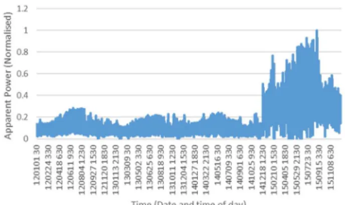
Where znorm is the normalized value, z is the variable being normalized, zmin and zmax are the minimum and maximum variable values, respectively. The loading data were as normalized in a single batch as opposed to normalizing the data in batches as in [37]. The station’s normalized raw loading data are shown in Fig. 6. The time values are given in the yymmdd and hhmm format, respectively, for the date and time of day, for the period above. Dips were observed in the loading data. These dips resulted from the station’s normal operation and/or trips which led to the station being without power. The data were cleaned up to remove these dips and then normalized. Cleaning up data can be cumbersome and time-consuming. Hence, the need to investigate the effect of uncleaned data on the AI models' performance. The cleaned up data plot is shown in Fig. 7. The models were trained and tested using two different subsets of the collected data for winter periods in the same years, but different periods. The load forecasting
2 VOLUME XX, 2017 experiments were conducted using MATLAB. The
temperature data were obtained from the South African weather services. The temperature data used were from a weather station in a neighboring town approximately 30km away from the substation under study. These were the closest available temperature data. The temperature data were also normalized using (20).
2) CASE STUDY B SUBSTATION AND DISTRIBUTION
NETWORK OVERVIEW
The substation in the second Case Study is located in a separate network to that in Case Study A, but in a nearby geographic location, in a neighboring town. This town is approximately 30 km away from the town the substation in Case Study A is located in. The temperature data used in this study were taken from a weather station in this town. This was the closest weather station to both substations in this study. The customer’s loading data used were from the power meter installed at the redistributor customer’s point of supply. The customer is supplied power at a voltage of
132 kV. This customer is connected to the power grid via a 400/132 kV transmission substation. The transmission substation also supplies other 132 kV substations and distribution (Dx.) networks. A switching substation connects the customer to the transmission substation. A switching substation is a substation that does not have transformers. The customer has a substation on its side with transformers to step the voltage down for distribution. The overview of the distribution network the substation under study in Case Study B is located in is shown in Fig. 5. The loading data for this customer were also stored as 30 minutes average power consumption. The data also had dips that were cleaned out as in Case Study A. The cleaned and non-cleaned data sets were also normalized using (20). The plots of the raw and cleaned data are presented in Fig. 8 and Fig. 9, respectively. From the data, it can be seen that the power consumption increased dramatically from around January 2015.
FIGURE 4. Distribution network the substation in Case Study A is located
FIGURE 5. Distribution network the substation in Case Study B is located
275 kV Tx substation bus-bar 132 kV Transmission (Tx) substation bus-bar 132 kV Dx Network 88 kV D x Ne tw or k Transformer set 1 Transformer set 2 132kV Dx substation 132kV Dx substation Power Measuring Device
88/11 kV Substation Under Study
88 kV Transmission (Tx) substation bus-bar
VOLUME XX, 2017 9
FIGURE 6. Raw normalized loading data for the distribution substation
in Case Study A
FIGURE 7. Cleaned-up normalized loading data for the distribution
substation in Case Study A
FIGURE 8. Raw normalized loading data for the distribution substation
in Case Study B
FIGURE 9. Cleaned-up normalized loading data for the distribution
substation in Case Study B
This growth in power consumption can be attributed to an increase in the number of electrical connections due to electrification and an increase in illegal connections, etc. The experiments in this Case Study were also separated into those with cleaned and non-cleaned loading data, and further sub-experiments with and without temperature as an input variable, respectively. The same temperature data used for Case Study A were also used in this Case Study
B. EXPERIMENT SETUP
The experiments were set up into two main sets. One set of experiments had models that were developed with the uncleaned loading/power consumption data. The second experiments set was with models developed with cleaned loading data. Both experiments sets were divided into two sub-experiment types based on two different input variables groups. Input variables group 1 excluded the geographic temperature data for where the station is located. Input variables group 2, included temperature data corresponding to the utilized input power consumption data. This input variables’ grouping enabled the understanding of the impact of temperature on the AI models’ load forecasting performance. The South African winter period was used for the experiments and a two-week ahead test load forecasting period was used. The rationale for choosing the winter period was that the utility’s maintenance departments focus on distribution maintenance execution during this time. This preference is mainly due to low rainfall and thunderstorms experienced in this period. These conditions provide multiple benefits, such as ease of performing work in non-rainy conditions, ease of navigation on mountainous areas and gravel roads, low risk of lightning strikes, etc. The South African winter period falls between 1 June and 31 August. The utility engineers gave two weeks as a sufficient period to plan maintenance. The two input variables groups are presented in Table I. A variable indicating whether the load corresponds to a peak period or non-peak period was also part of the input variables. The peak periods used for winter in this research were 06:00 to 09:00 for the morning peak and 18:00 to 21:00 for the evening peak. Each of these variables was in 30 minutes intervals, for a period of two weeks. The
VOLUME XX, 2017 9 training input matrices were thus 672×5 for models trained
with input variable Group 1 and 672×8 for models trained with input variable Group 2. After training, the models were tested for the winter period using a test data set. The test data set’s input and target values were respectively different from those of the training data set. The results in the next section are for a two-week ahead load forecast using the test data set. These test load forecasting results are for a two-week time series.
TABLEI INPUT VARIABLES GROUPS
Input variables
group
Inputs
Group 1 Power consumption two years before the forecast period, Time of day,
Peak or non-peak period indicator,
Power consumption a year before the forecast period, Power consumptiontwo weeks before the forecast period, Group 2 Power consumption two years before the forecast,
Temperature two years before the forecast, Time of day,
Peak or non-peak period indicator,
Power consumption a year before the forecast, Temperature one year before the forecast, Power consumption two weeks before the forecast, Temperature two weeks before the forecast period
V. EXPERIMENT RESULTS
This section presents the load forecasting performance results for the three techniques' models. The three performance measures used to measure the different models' performance in this research are also presented.
A. PERFORMANCE MEASURES USED IN THIS STUDY
The performance of the AI models was measured using three error measurements. These measurements are the symmetric mean absolute percentage error (sMAPE), mean absolute error (MAE) and root mean square error (RMSE) and are respectively given by (21), (22) and (23):
s+t = ∑ |vw2:w|
|vw|x|:w|
E (21)
s+ =∑Bw |vw2Iw| (22) ysz = {∑Bw (vw2:w)5 (23) where Fk is the kth forecast value, Tk is the kth target value and N is the total number of forecasts. The results are summarized in the subsections below. The sMAPE as written in (21) spans between 0% and 200%, after multiplication by 100%. To get the value between 0% and 100%, the 2 in the equation is removed before multiplication by 100%.
B. ANFIS EXPERIMENTAL RESULTS
Using a trial and error approach, multiple ANFIS tuning parameters were experimented with. These parameters
determine the number of rules, the rules, the membership functions and the overlaps between the membership functions. The maximum training number of epochs and acceptable training error (RMSE) were kept constant at 150 and 0.0001, respectively, for the development of all the models. For most of the models, the training error stopped decreasing before reaching the 100th training epoch. The
models’ performanceresults are given in Table II to Table V for each of the two sub-experiments with raw and cleaned loading data using four ANFIS tuning parameters. The results attained with other tuning parameters were given similar rules and a similar number of rules, and hence similar results to the results recorded in Table II to Table V. This subsection discusses the results from the two Case Studies.
1) CASE STUDY A ANFIS RESULTS
The ANFIS models’ load forecast results showed that the errors attained with models developed with raw/non-cleaned data were lower than those with raw/non-cleaned loading data. The results with the lowest error were achieved with input variables Group 1 and the 3rd tuning parameters
respectively. These results are bolded in Table II. The models developed with the raw data showed lower errors than models developed with cleaned up data. The model with the lowest error had an sMAPE of 0.138483, MAE of 0.052392 and RMSE of 0.071799. The model, developed with cleaned loading data, which achieved the lowest error achieved an sMAPE of 0.207322, MAE of 0.059294 and RMSE of 0.081476. It is thus observed that the load forecasting error without inclusion of temperature in the development of the AI models can be lower than when temperature is included.
2) CASE STUDY B ANFIS RESULTS
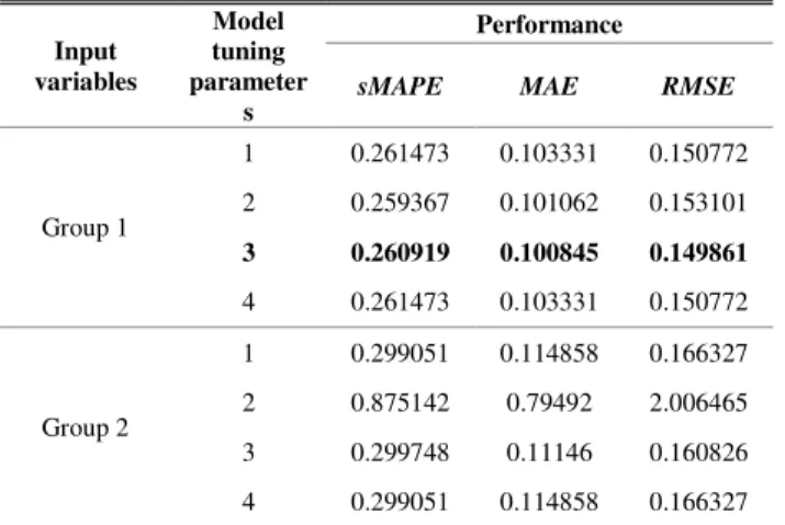
The results show that the error was lower with cleaned loading data. The lowest error results were attained without the use of temperature in the development of ANFIS models with both cleaned and uncleaned data. The performance of the ANFIS models' two-week ahead load forecasts are given in Table IV and Table V. The lowest attained error was an sMAPE of 13.05%, MAE of 10.09% and RMSE of 14.99%, and is bolded in Table V.
C. OP-ELM EXPERIMENTAL RESULTS
Optimally pruned extreme learning machine models were developed, and then tested using the testing data. The effect of model dimensions on the load forecasting performance was studied. That is, the models’ number of hidden nodes were adjusted for the different models that were developed. The model’s final dimensions were determined through the LOO method. Hence, a certain number of hidden units may at times not be attainable. The models’ performance was then captured for two-week ahead load forecasts. The models here were trained to solve a regression problem as
VOLUME XX, 2017 9 load forecasting is a regression problem. The results are
presented and discussed in this subsection. TABLEII
CASE STUDY AANFISEXPERIMENTS RESULTS WITH RAW LOADING DATA
Input variables Model tuning parameter s Performance
sMAPE MAE RMSE
Group 1 1 0.1495145 0.0567013 0.0804968 2 0.17506 0.066914 0.092543 3 0.138483 0.052392 0.071799 4 0.1495145 0.0567013 0.0804968 Group 2 1 0.1836643 0.0696844 0.0920817 2 0.177639 0.068296 0.092137 3 0.162643 0.05886 0.07956 4 0.1968307 0.0728959 0.0964678 TABLEIII
CASE STUDY AANFISEXPERIMENTS RESULTS WITH CLEANED LOADING DATA Input variables Model tuning parameter s Performance
sMAPE MAE RMSE
Group 1 1 0.226631 0.064804 0.092812 2 0.279851 0.078866 0.109888 3 0.207322 0.059294 0.081476 4 0.226631 0.064804 0.092812 Group 2 1 0.280986 0.079 387 0.104689 2 0.27447 0.078297 0.104904 3 0.243374 0.066815 0.090639 4 0.295661 0.079239 0.105947 TABLEIV
CASE STUDY BANFISEXPERIMENTS RESULTS WITH RAW LOADING DATA
Input variables Model tuning parameter s Performance
sMAPE MAE RMSE
Group 1 1 0.3280877 0.1244868 0.1763246 2 0.3548188 0.1181713 0.1698449 3 0.3485234 0.1591555 0.3033930 4 0.356657 0.128948 0.182569 Group 2 1 0.509364 0.184724 0.272112 2 0.919458 0.765156 1.386215 3 0.4223565 0.1656288 0.2677004 4 0.470634 0.179244 0.26091 TABLEV
CASE STUDY BANFISEXPERIMENTS RESULTS WITH CLEANED LOADING DATA Input variables Model tuning parameter s Performance
sMAPE MAE RMSE
Group 1 1 0.261473 0.103331 0.150772 2 0.259367 0.101062 0.153101 3 0.260919 0.100845 0.149861 4 0.261473 0.103331 0.150772 Group 2 1 0.299051 0.114858 0.166327 2 0.875142 0.79492 2.006465 3 0.299748 0.11146 0.160826 4 0.299051 0.114858 0.166327
1) CASE STUDY A OP-ELM RESULTS
In all cases with the different input parameters for cleaned and raw data, the models showed higher accuracies when their dimensions were smaller. It was again observed that the models trained with raw data had lower test errors in comparison to those trained with cleaned up data, as with ANFIS models. The experiment results are summarized in Table VI and Table VII.
TABLEVI
CASE STUDY AOP-ELMEXPERIMENTS RESULTS WITH RAW LOADING DATA Input variables Hidden Nodes Performance
sMAPE MAE RMSE
Group 1 10 0.1315575 0.0491749 0.0657673 55 0.1406914 0.0528443 0.0721915 80 0.1542054 0.0568670 0.0779820 100 0.1645267 0.0592804 0.0812588 Group 2 8 0.1364757 0.0511859 0.0682780 58 0.1596773 0.0587954 0.0754893 103 0.1484154 0.0552860 0.0712436 158 0.1793395 0.0681535 0.0885394
2) CASE STUDY B OP-ELM RESULTS
The load forecasting performance of OP-ELM models is presented in Table VIII to Table IX. It was observed that, with both raw and cleaned loading data, the lowest errors were attained with a lower number of hidden nodes in the hidden layer. This was with models developed without the use of temperature in the input variables. With the lowest error achieved by a model with 10 hidden nodes and developed with cleaned loading data. This model achieved an sMAPE of 0.226413 (11.32%), MAE of 0.09043 (9.04%) and RMSE of 0.143772 (14.38%). Models with 100 and 110 hidden nodes could not be attained with cleaned loading data when temperature was not used as an input variable.
VOLUME XX, 2017 9
D. LSTM EXPERIMENTAL RESULTS
The LSTM models were trained using the Adam optimizer. The number of hidden units were varied for each model’s training. The models here were also trained to solve a regression problem. The other parameters such as learning rate, maximum epochs, etc. were kept constant. The results for the two case studies are presented and discussed in this subsection.
1) CASE STUDY A LSTM RESULTS
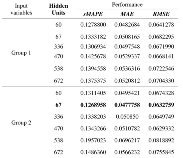
The LSTM results showed that more hidden units do not necessarily lead to an increase in the model's accuracy. The LSTM results are presented in Table X and Table XI. The lowest error was attained when the number of hidden units was 67. The models trained with raw data gave lower test errors than models trained with cleaned data.
TABLEVII
CASE STUDY AOP-ELMEXPERIMENTS RESULTS WITH CLEANED LOADING DATA Input variables Hidden Nodes Performance
sMAPE MAE RMSE
Group 1 10 0.2014222 0.0562507 0.0752450 50 0.2171528 0.0601624 0.0818262 100 0.2294828 0.0617002 0.0826178 110 0.2319736 0.0641421 0.0835023 Group 2 8 0.2004182 0.0564162 0.0759865 58 0.2264838 0.0629379 0.0841188 108 0.2645317 0.0714689 0.0917274 158 0.2996661 0.0777273 0.0992270 TABLEVIII
CASE STUDY BOP-ELMEXPERIMENTS RESULTS WITH RAW LOADING DATA Input variables Hidden Nodes Performance
sMAPE MAE RMSE
Group 1 10 0.279146 0.105113 0.16436 55 0.375057 0.156518 0.232913 80 0.515501 0.229931 0.38793 100 0.483081 0.221968 0.396976 Group 2 8 0.285174 0.106607 0.161916 58 0.410711 0.144622 0.203808 103 0.578441 0.208359 0.275639 158 0.595474 0.212417 0.312686 The models trained with weather temperature could forecast the load slightly lower errors than models trained without the temperature. This observation could be because of deep learning techniques' ability to learn more features and tendency to achieve higher accuracies with more data in their training.
TABLEIX
CASE STUDY BOP-ELMEXPERIMENTS RESULTS WITH CLEANED LOADING DATA Input variables Hidden Nodes Performance
sMAPE MAE RMSE
Group 1 10 0.226413 0.09043 0.143772 50 0.347886 0.22436 0.482956 100 - - - 110 - - - Group 2 8 0.235541 0.092093 0.141977 58 0.281593 0.108865 0.169301 108 0.376353 0.149048 0.232213 158 0.626704 0.213157 0.29973 TABLEX
CASE STUDY ALSTMEXPERIMENTS RESULTS WITH RAW LOADING DATA
Input variables
Hidden Units
Performance
sMAPE MAE RMSE
Group 1 60 0.1278800 0.0482684 0.0641278 67 0.1333182 0.0508165 0.0682295 336 0.1306934 0.0497548 0.0671990 470 0.1425678 0.0529337 0.0668141 538 0.1394558 0.0536316 0.0722546 672 0.1375375 0.0520812 0.0704330 Group 2 60 0.1311405 0.0495421 0.0674328 67 0.1268958 0.0477758 0.0632759 336 0.1338203 0.050850 0.0649749 470 0.1343266 0.0510782 0.0629332 538 0.1957023 0.0696217 0.0818892 672 0.1486360 0.0566232 0.0755845
2) CASE STUDY B LSTM RESULTS
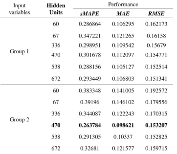
The load forecasting performance of the LSTM models developed with uncleaned and cleaned data is given in Table XII and Table XIII, respectively. The inclusion of temperature in the development of LSTM models generally led models with both cleaned and uncleaned data. These results are bolded in Tables XII and XIII, respectively. Here a model developed with cleaned loading data attained the lowest load forecasting error. This performance was an sMAPE of 0.2307 (11.54%), MAE of 0.0896 (8.96%) and RMSE of 0.14065 (14.07%).
VOLUME XX, 2017 9 TABLEXI
CASE STUDY ALSTMEXPERIMENTS RESULTS WITH CLEANED LOADING
DATA Input variables Hidden Units Performance
sMAPE MAE RMSE
Group 1 60 0.2076085 0.0605033 0.0817285 67 0.2144895 0.0626986 0.0843537 336 0.2011207 0.0563641 0.0733492 470 0.2540580 0.0748961 0.0936343 538 0.2235020 0.0638470 0.0837461 672 0.2127313 0.0595342 0.0764751 Group 2 60 0.1909078 0.0533111 0.0695006 67 0.1916753 0.0546699 0.0739185 336 0.2071473 0.0585931 0.0787505 470 0.2076085 0.0605033 0.0817285 538 0.2144895 0.0626986 0.0843537 672 0.2011207 0.0563641 0.0733492 TABLEXII
CASE STUDY BLSTMEXPERIMENTS RESULTS WITH RAW LOADING DATA
Input variables
Hidden Units
Performance
sMAPE MAE RMSE
Group 1 60 0.286864 0.106295 0.162173 67 0.347221 0.121265 0.16158 336 0.298951 0.109542 0.15679 470 0.301678 0.112097 0.154771 538 0.288156 0.105127 0.152514 672 0.293449 0.106803 0.151341 Group 2 60 0.383348 0.141005 0.192572 67 0.39196 0.146102 0.179556 336 0.344087 0.122243 0.170315 470 0.263784 0.098621 0.153207 538 0.291305 0.10337 0.152825 672 0.32681 0.121577 0.159715
E. MODELS' RESULTS COMPARISON AND
DISCUSSION
In Case Study A, deep neural networks, LSTM, had the lowest test errors in comparison to ANFIS and OP-ELM. All techniques were observed to have the lowest test errors when using raw data. The inclusion of the temperature in the input variables was observed to reduce the load forecasting error in LSTM models. ANFIS and OP-ELM were observed to achieve lower errors without the inclusion of temperature in their models’ training data. The difference in the lowest test errors sMAPE, MAE and RMSE, for the respective models’ cases, with and without temperature, was within a 2% margin. The lowest attained error results in Case Study A, for
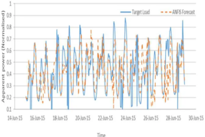
each of the three techniques are summarized in Table XIV. Fig. 10., Fig. 11. and Fig. 12. show the investigated techniques' models' 2-week ahead load forecast test results against the target load profile for their lowest attained errors in Case Study A. The models achieved lower errors with the uncleaned loading data. The loading data can, therefore, be used without being cleaned up to train AI models to forecast distribution network loads similar to those in Case Study A. Depending on the error that the user can tolerate the hybrid AI techniques used in this research can be deployed to forecast load without temperature data. LSTM can also be deployed without temperature. This statement is said following the observation that the errors attained by LSTM without temperature as an input variable were still lower than those attained by ANFIS and OP-ELM
TABLEXIII
CASE STUDY BLSTMEXPERIMENTS RESULTS WITH CLEANED LOADING
DATA Input variables Hidden Units Performance
sMAPE MAE RMSE
Group 1 60 0.258684 0.102794 0.156705 67 0.278574 0.107823 0.152683 336 0.356105 0.139668 0.167961 470 0.265542 0.099076 0.149288 538 0.340204 0.132768 0.171631 672 0.24577 0.101353 0.152643 Group 2 60 0.251145 0.100358 0.155083 67 0.272416 0.102874 0.153517 336 0.242085 0.094544 0.143096 470 0.299866 0.114675 0.146952 538 0.412537 0.171554 0.208968 672 0.230693 0.089595 0.14065
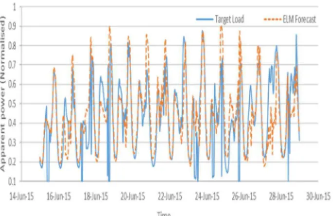
In Case Study B all the techniques’ models achieved their lowest errors when cleaned loading data were used to develop their load forecasting models. These models’ lowest attained error results are presented in Table XV. LSTM achieved the lowest load forecasting error amongst the three techniques used. This performance was an sMAPE of 0.2307 (11.54%), MAE of 0.0896 (8.96%) and RMSE of 0.14065 (14.07%). LSTM achieved this performance with a model developed with input variables group 2. The two hybrid AI techniques, ANFIS and OP-ELM, achieved their best performance with input variable group 1, which did not have temperature as one of the input variables. ANFIS had the lowest accuracy in comparison to the other two techniques used. Fig. 13. to Fig. 15. show the three techniques’ models’ two-week ahead load forecast test results which gave the lowest error plotted against the target load.
VOLUME XX, 2017 9 LSTM was found to lead to a model with the lowest error
in both Case Study A and Case Study B. In both cases LSTM models achieved this performance when temperature was used in the model’s development. ANFIS models’ highest achieved accuracy was lower than the highest achieved accuracy by the other two techniques’ models. It can therefore be concluded that the inclusion of temperature in the development of DL load forecasting models for Dx redistributor loads improves their forecasting accuracy. Hybrid AI techniques’ models’ load forecasting accuracy decreased with the inclusion of temperature in their development. The main difference in the two cases is that the models in Case Study A attained their highest load forecasting accuracy with non-cleaned data, as opposed to cleaned data in Case Study B. The combination of the steep change in loading and the number of data points that required cleaning up may be a cause for this. The cause of this difference can be investigated further.
TABLEXIV
SUMMARY OF THE LOWEST ERRORS ATTAINED FROM EACH OF THE 3 INVESTIGATED TECHNIQUES IN CASE STUDY A
(ALL ATTAINED WITH RAW DATA) Technique Input
variables
Performance
sMAPE MAE RMSE
ANFIS Group 1 0.138483 0.052392 0.071799 OP-ELM Group 1 0.1315575 0.0491749 0.0657673
RNN-LSTM Group 2 0.1268958 0.0477758 0.0632759
TABLEXV
SUMMARY OF THE LOWEST ERRORS ATTAINED FROM EACH OF THE 3 INVESTIGATED TECHNIQUES IN CASE STUDY B
(ALL ATTAINED WITH CLEANED DATA) Technique Input
variables
Performance
sMAPE MAE RMSE
ANFIS Group 1 0.260919 0.100845 0.149861 OP-ELM Group 1 0.226413 0.09043 0.143772
RNN-LSTM Group 2 0.230693 0.089595 0.14065
FIGURE 10.Case Study AANFIS 2-week load forecast results versus the
target raw data normalized load
FIGURE. 11. Case Study A OP-ELM 2-week load forecast results versus
the target raw data normalized load
FIGURE 12. Case Study A LSTM-RNN 2-week load forecast results
versus the target raw data normalized load
FIGURE. 13. Case Study B ANFIS 2-week load forecast results versus
the target raw data normalized load
0.1 0.2 0.3 0.4 0.5 0.6 0.7
14-Jun-15 16-Jun-15 18-Jun-15 20-Jun-15 22-Jun-15 24-Jun-15 26-Jun-15 28-Jun-15 30-Jun-15
A p p a r e n t p o w e r ( N o r m a l i s e d ) Time
Target ANFIS Forecast
0.1 0.2 0.3 0.4 0.5 0.6 0.7
14-Jun-15 16-Jun-15 18-Jun-15 20-Jun-15 22-Jun-15 24-Jun-15 26-Jun-15 28-Jun-15 30-Jun-15
A p p a r e n t p o w e r ( N o r m a l i s e d ) Time
Target ELM Forecast
0.1 0.2 0.3 0.4 0.5 0.6 0.7
14-Jun-15 16-Jun-15 18-Jun-15 20-Jun-15 22-Jun-15 24-Jun-15 26-Jun-15 28-Jun-15
A p p a r e n t p o w e r ( N o r m a l i s e d ) Time Target LSTM Forecast
VOLUME XX, 2017 9
FIGURE. 14. Case Study B OP-ELM 2-week load forecast results versus
the target raw data normalized load
FIGURE 15. Case Study B LSTM-RNN 2-week load forecast results
versus the target raw data normalized load
VI. CONCLUSIONS
This paper presented a novel hybrid AI and deep learning distribution load forecasting system. The system was used to introduce and investigate a state of the art hybrid artificial intelligence technique and a deep learning technique, OP-ELM and LSTM, respectively, in SA distribution networks load forecasting. Two real South African distribution redistributor customer's power consumption data were used for the twocase studies. The first Case Study was an 88/11 kV, 80 MVA substation, with two 40 MVA transformers. The second Case Study, Case Study B, was a customer supplied through a 132 kV switching substation. The impact of temperature on the performance of a recent state-of-the-art hybrid AI technique's and DL technique's models was also investigated. ANFIS and OP-ELM were found to achieve higher levels of accuracies without the inclusion of temperature in the development of their models in both case studies. It was the opposite for LSTM, whose models achieved their lowest errors with the inclusion of temperature in their development. The lowest load forecasting error by an LSTM model in the Case Study A was ansMAPE of 6.35%, MAE of 4.78% and RMSE of 6.33%. The best LSTM model’s performance in Case Study B was an sMAPE of 11.54%, MAE of 8.96% and RMSE of 14.07%. It was
observed that the long short-term memory had a forecasting error lower than adaptive neuro-fuzzy logic and optimally pruned extreme learning machines in both cases. The cleaning up of loading data to remove spikes and dips led to reduced accuracies in all technique's corresponding models in Case Study A. The opposite was the case in Case Study B. The effect of other weather parameters such as humidity, rain, wind, etc. when using deep learning techniques in South African distribution network's load forecasting should be explored further. This is following the load forecasting performance of LSTM models developed with temperature as one of the input variables. This study showed that recent hybrid AI techniques and deep learning techniques can be used in South African distribution load forecasting. The techniques can be further explored on medium-voltage (MV) distribution reticulation networks load forecasting and bulk power supplied, large power users. South Africa is still lagging behind in the rollout of smart meters, hence future work should look at the incorporation of smart meters to improve load forecasting in distribution networks. The study of the impact of customers' behavior in demand response on the load forecasting performance of hybrid AI and deep learning techniques may also need to be studied in the future. This study should include the incorporation of smart meter data.
REFERENCES
[1] J.P. Holloway, P. Mokilane, S. Makhanya, T. Magadla and R. Koen, "Forecast of electricity demand in South Africa (2014 - 2050) using CSIR sectoral regression model," CSIR, 2016. [Online]. Available: http://www.energy.gov.za/IRP/2016/IRP-AnnexureB-Demand-forecastsreport.. [Accessed 2019 April 2]. [2] M. Mashao, "Trends in the consumption of electricity in
the industry RSA perspective," Eskom, 2012. [Online]. Available:
http://www.energy.gov.za/files/IEP/presentations/Trends InTheConsump. [Accessed 02 April 2019].
[3] World energy outlook, "Morden energy for all,"
[Online]. Available:
http://www.worldenergyoutlook.org/resources/energyde velopment/. [Accessed August 2018].
[4] M. Kanagawa and T. Nakata, "Assessment of access to electricity and socio-economic impacts in rural areas of developing countries," Energy policy, vol. 36, no. 6, p. 2016 – 2029, 2008.
[5] H. Winkler, A.F. Simões, E.L La Rovere, M. Alam, A. Rahman and S. Mwakasonda, "Access and affordability of electricity in developing countries," World development, vol. 39, no. 6, pp. 1037-1050, 2011.
VOLUME XX, 2017 9 [6] C.N.H. Doll and S. Pachauri, "Estimating rural
populations without access to electricity in developing countries through night-time light satellite imagery," Energy policy, vol. 36, no. 10, p. 5661 – 5670, 2010. [7] G. Prasad, "South African electrification programme,"
Global network on energy for sustainable development (GNESD), [Online]. Available: http://energyaccess.gnesd.org/cases/22-south-african-electrification-programme.html. [Accessed 02 April 2019].
[8] South African Government, "Integrated national electrification programme," South African Government,
[Online]. Available:
http://www.gov.za/aboutgovernment/government-programmes/inep. [Accessed 03 February 2019]. [9] L. Marwala and B. Twala, "Forecasting electricity
consumption in South Africa: ARMA, Neural networks and Neurro-fuzzy," in International joint conference on Neural Networks, Beijing, 2014.
[10]E. Ceperic, V. Ceperic and A. Baric, "A strategy for short-term load forecasting by support vector regression machines," IEEE Transaction on Power Systems, vol. 28, no. 4, pp. 4356 - 4364, 2013.
[11]E.A. Feinberg and D. Genethliou, "Load forecasting," in In: J.H. Chow, F.F. Wu, J. Momoh. (eds), Applied Mathematics for Restructured Electric Power Systems. Power Electronics and Power Systems, Boston, MA, Springer, 2005, pp. 269-285.
[12]W. Kong, Z. Y. Dong, D. J. Hill, F. Luo and Y. Xu, "Short-term residential load forecasting based on resident behaviour learning," IEEE Transactions on Power Systems, vol. 33, no. 1, pp. 1087-1088, 2018. [13]S. Welikala, C. Dinesh, M.P.B. Ekanayake, R. I.
Godaliyadda and J. Ekanayake, "Incorporating appliance usage patterns for non-intrusive load monitoring and load forecasting," IEEE TRANSACTIONS ON SMART GRID, vol. 10, no. 1, pp. 448-461, 2019.
[14]W. Kong, Z. Y. Dong, Y. Jia, D. J. Hill, Y. Xu and Y. Zhang, "Short-term residential load forecasting based on LSTM recurrent neural network," IEEE Transactions on Smart Grid, vol. 10, no. 1, pp. 841-851, 2019.
[15]R. G. Rajasekaran, S. Manikandaraj and R. Kamaleshwar, "Implementation of machine learning algorithm for predicting user behavior and smart energy management," in 2017 International Conference on Data Management, Analytics and Innovation (ICDMAI), Pune, India, 2017.
[16]D. Liu, Y. Sun, Y. Qu, B. Li and Y. Xu, "Analysis and accurate prediction of user's response behavior in incentive-based demand response," IEEE Access, vol. 7, pp. 3170-3180, 2019.
[17]B. Zeng, X. Wei, D. Zhao, C. Singh and J. Zhang, "Hybrid probabilistic-possibilistic approach for capacity credit evaluation of demand response considering both
exogenous and endogenous uncertainties," Applied Energy, vol. 229, pp. 186-200, 2018.
[18]X. Zhou, N. Yu, W. Yao and R. Johnson, "Forecast load impact from demand response resources," in 2016 IEEE Power and Energy Society General Meeting (PESGM), Boston, MA, USA, 2016.
[19]L. Han, Y. Peng, Y. Li, B. Yong, Q. Zhou and L. Shu, "Enhanced deep networks for short-term and medium-term load forecasting," IEEE Access, vol. 7, pp. 4045-4055, 2019.
[20]R.F. Berriel, A.T. Lopes, A. Rodrigues, F.M. Varejão and T. Oliveira, "Monthly energy consumption forecast a deep learning approach," in International Joint Conference on Neural Networks (IJCNN), 2017. [21]G. M. U. Din and A.K. Marnerides, "Short term power
load forecasting using deep neural networks," in International Conference on Computing, using deep neural networks, 2017.
[22]F. Fahiman, S.M. Erfani, S. Rajasegarar, M. Palaniswami and C. Leckie, "Improving load forecasting based on deep and k-shape clustering," in International Joint Conference on Neural Networks (IJCNN), Anchorage, AK, USA, 2017.
[23]X.W Chen and X Lin, "Big data deep learning: Challenges and perspectives," IEEE Access, vol. 2, pp. 514-525, 2014.
[24]N. Nguyen and S. Lee, "Robust Boundary Segmentation in Medical Images Using a Consecutive Deep Encoder-Decoder Network," in IEEE Access, vol. 7, pp. 33795-33808, 2019
[25]N. Majumder, S. Poria, A. Gelbukh and E. Cambria, "Deep learning-based document modeling for personality detection from text," IEEE Intelligent Systems, vol. 32, no. 2, pp. 74-79, 2017.
[26]S. Albarqouni, C. Baur, F. Achilles, V. Belagiannis, S. Demirci and N. Navab, "AggNet: Deep learning from crowds for mitosis detection in breast cancer histology images," IEEE Transactions on medical imaging, vol. 35, no. 5, pp. 1313-1321, 2016.
[27]J.M. Martín-Doña, A.M. Gomezs, J.A. Gonzalez and A.M. Peinado, "A deep learning loss function based on the perceptual evaluation of the speech quality," IEEE Signal processing letters, vol. 25, no. 11, pp. 1680-1684, 2018.
[28]A. Narayan and K.W. Hipel, "Long short term memory networks for short-term electric load forecasting," in IEEE International conference on systems, man and cybernetics (SMC), 2017.
[29]W. Yin, K. Kann, M. Yu and H. Schütze, "Comparative Study of CNN and RNN for Natural Language Processing," in Computing research repository (CoRR), abs/1702.01923,, 2017.
VOLUME XX, 2017 9 [30]Z. Yu, W. T. Z. Niu and Q. Wu, "Deep learning for daily
peak load forecasting a novel gated recurrent neural network combining dynamic time warping," IEEE Access, vol. 7, pp. 17184-17194, 2019.
[31]P. Dehghanian, B. Zhang, T. Dokic and M. Kezunovic, "Predictive risk analytics for weather-resilient operation of electric power systems," IEEE Transactions On Sustainable Energy, vol. 10, no. 1, pp. 3-15, 2019. [32]L. Marwala and B. Twala, "Causality Tests Using Basic
and Optimally-Pruned Extreme Learning Machines," in 2nd International Conference on Control and Robotics Engineering, Bangkok, Thailand, 2017.
[33]L. Marwala and B. Twala, "Electricity load forecasting using an ensemble of optimally-pruned and basic extreme learning machines," in 9th IEEE-GCC Conference and Exhibition (GCCCE), Manama, Bahrain, 2017.
[34]N.M Ijumba and J.P. Hunsley, "Improved load forecasting techniques for the newly electrified areas," in IEEE Africon conference in Africa, Cape Town, South Africa, 1999.
[35]W. Yuill, R. Kgokong, S. Chowdhury and S.P. Chowdhury, "Application of adaptive neuro fuzzy inference system (ANFIS) based short term load forecasting in South African power networks," in 45th International Universities Power Engineering Conference UPEC2010, Cardiff, Wales, 2010.
[36]W. Yuill, R. Kgokong, S. P. Chowdhury and S. Chowdhury, "Management of short term load forecasting in South African power networks," in 2010 International Conference on Power System Technology, Hangzhou, China, 2010.
[37]S. Motepe, A. N. Hasan and R. Stopforth, "South African distribution networks load forecasting using ANFIS," in IEEE Power Electronics Drivers and Energy Systems (PEDES) Conference, 2018.
[38]S. Motepe, A. N. Hasan, B. Twala and R. Stopforth, "Power distribution networks load forecasting using deep belief networks: The South African case," in IEEE Jordan International Joint Conference on Electrical Engineering and Information Technology, Amman, Jordan, 2019.
[39]L.K. Tartibu and K.T. Kabengele, "Forecasting net energy consumption of South Africa using artificial neural network," in 2018 International Conference on the Industrial and Commercial Use of Energy (ICUE), Cape Town, South Africa, 2018.
[40]L. Marwala and B. Twala, "Univariate modeling of electricity consumption in South Africa: neural networks and neuro-fuzzy systems," in IEEE International conference on systems, man and cybernetics, 2013. [41]M. Negnevitsky, Artificial intelligence: A guide to
intelligent systems 2nd Edition, United Kingdom: Addison-Wesley, 2005.
[42]S. Motepe, B. Twala, Q-G Wang and R. Stopforth, "Determining distribution power system loading measurements accuracy using fuzzy logic," Procedia Manufacturing, vol. 7, pp. 435-439, 2017.
[43]J. Kacprzyk and W. Pedrycz, Springer handbook of computational intelligence, Berlin, Germany: Springer, 2015.
[44]M. Rejc and M. Pantos, "Short term transmission-loss forecast for the Slovenian transmission power system based on fuzzy-logic decision approach," IEEE Transactions on Power Systems, vol. 26, no. 3, pp. 1511-1521, 2011.
[45]G. Tso and K. Yau, "Predicting electricity consumption: A comparison of regression analysis, decision tree and neural networks," Energy, vol. 32, pp. 1761-1768, 2007. [46]H.D. Block, "The perceptron: a model for brain functioning," Reviews of Modern Physics, vol. 34, no. 1, pp. 123-135, 1962.
[47]A.N. Hasan, B. Twala and T. Marwala, "Predicting mine dam levels and energy consumption using artificial intelligence methods," in IEEE Symposium on Computational Intelligence for Engineering Solutions, Singapore, 2013.
[48]A. Ali and A. N. Hasan, "Improving single classifiers prediction accuracy for underground water pump station in a gold mine using ensemble techniques," in IEEE International Conference on Computer as a Tool (EUROCON), 2015.
[49]L.J. Mpanza and T. Marwala, "Artificial neural network and rough set for HV bushings condition monitoring," in 15th International Conference on Intelligent Engineering Systems, Poprad, Slovakia, 2011.
[50]A. Ali and A. N. Hasan, "Optimization of PV model using fuzzy-neural network for DC-DC converter systems," in 2018 9th International Renewable Energy Congress (IREC), Hammamet, Tunisia, 2018.
[51]A. M. Farayola, A. N. Hasan and A. Ali, "Curve fitting polynomial technique compared to ANFIS technique for maximum power point tracking," in 8th International Renewable Energy Congress (IREC), 2017.
[52]J.L. McClelland and D.E. Rumelhart, Parallel distributed processing: Explorations in the microstructure of cognition, Vol. 2: Psychological and biological models, Cambridge, MA, USA: MIT Press, 1986.
[53]S. Motepe, B. Twala and R. Stopforth, "Determining South African distribution power system big data integrity using fuzzy logic: Power measurements data application," in 2017 Pattern Recognition Association of South Africa and Robotics and Mechatronics, Bloemfontein, South Africa, 2017.
[54]Y. Miche, A. Sorjamaa and A. Lendasse, "OP-ELM: Theory, experiments and a toolbox," in 18th International Conference on Artificial Neural Networks (ICANN), Prague, Czech Republic, 2008.
VOLUME XX, 2017 9 [55]G.B. Huang, Q.Y. Zhu and C. Siew, "Extreme learning
machine: Theory and applications," Neurocomputing, vol. 70, no. 1-3, pp. 489-501, 2006.
[56]F. Wang, Z. Zhao, X. Li, F. Yu and H. Zhang, "Stock volatility prediction using multi-kernel learning based extreme learning machine," in International Joint Conference on Neural Networks (IJCNN), Beijing, China, 2014.
[57]X. Chen, Z.Y. Dong, K. Meng, Y. Xu, K.P. Wong and H.W. Ngan, "Electricity price forecasting with extreme learning machine and bootstrapping," IEEE Transactions on Power Systems, vol. 27, no. 4, pp. 2055-2062, 2012. [58]L. Marwala, Forecasting electricity demand in South
Africa using artificial intelligence, PhD. Thesis (Engineering),University of Johannesburg, 2015. [59]S. Hochreiter and J. Schmidhuber, "Long short-term
memory," Neural computation, vol. 9, no. 8, p. 1735– 1780, 1997.