Mathematics Theses Department of Mathematics and Statistics
5-2-2018
Influence Function-Based Empirical Likelihood
And Generalized Confidence Intervals For Lorenz
Curve
Yuyin Shi
Follow this and additional works at:https://scholarworks.gsu.edu/math_theses
This Thesis is brought to you for free and open access by the Department of Mathematics and Statistics at ScholarWorks @ Georgia State University. It has been accepted for inclusion in Mathematics Theses by an authorized administrator of ScholarWorks @ Georgia State University. For more information, please [email protected].
Recommended Citation
Shi, Yuyin, "Influence Function-Based Empirical Likelihood And Generalized Confidence Intervals For Lorenz Curve." Thesis, Georgia State University, 2018.
CONFIDENCE INTERVALS FOR LORENZ CURVE
by
YUYIN SHI
Under the Direction of Gengsheng Qin, PhD
ABSTRACT
This thesis aims to solve confidence interval estimation problems for Lorenz curve. First,
we propose new nonparametric confidence intervals with influence function-based empirical
likelihood method. It is shown that the limiting distributions of log-empirical likelihood
ratios are standard Chi-square distributions. Then the “exact” parametric intervals based on
generalized pivotal quantities for Lorenz ordinates are also developed. Extensive simulation
studies are conducted to evaluate the finite sample performance of the proposed methods.
Finally, our methods are applied on real income data sets.
INDEX WORDS: Empirical likelihood; Influence function; Generalized pivotal quantities; Lorenz ordinates.
CONFIDENCE INTERVALS FOR LORENZ CURVE
by
YUYIN SHI
A Thesis Submitted in Partial Fulfillment of the Requirements for the Degree of
Master of Science
in the College of Arts and Sciences Georgia State University
CONFIDENCE INTERVALS FOR LORENZ CURVE
by
YUYIN SHI
Committee Chair: Gengsheng Qin
Committee: Qi Xin Xiaoyi Min
Electronic Version Approved:
Office of Graduate Studies College of Arts and Sciences Georgia State University May 2018
DEDICATION
ACKNOWLEDGEMENTS
I would like to give my deep thanks and sincere gratitude to everyone for helping me complete this thesis.
First, I want to show my gratitude to my academic advisor, Dr. Gengsheng Qin, who has supported me throughout my thesis with his patience and knowledge. Dr. Qin gave me lots of suggestions and guidance while I was doing this thesis research, from the most basic language modification to the mathematical proof. His insight and knowledge always inspired me and I truly learned a lot from him.
I’d like to give my special thanks to my committee members, Dr. Xin Qi and Dr. Xiaoyi Min, for reviewing my thesis and their insightful comments and encouragement.
My gratitude also goes to Dr. Guantao Chen and Dr. Yichuan Zhao for their letters of recommendation to the Ph.D. programs I applied. To Dr. Jing Zhang, who gave wonderful lectures on different topics on statistics and biostatistics.
Special thanks to all the faculty, staff and students in the Department of Mathematics and Statistics at Georgia State University.
Last but not least, I would like to thank my parents, my uncle, my aunt, my boyfriend, my cousins and all my friends who helped me when I faced difficulties.
TABLE OF CONTENTS
ACKNOWLEDGEMENTS . . . v
LIST OF TABLES . . . viii
LIST OF FIGURES . . . ix
LIST OF ABBREVIATIONS . . . xi
CHAPTER 1 INTRODUCTION . . . 1
CHAPTER 2 EMPIRICAL LIKELIHOOD-BASED METHODS . . . 5
2.1 Influence Function-based Empirical Likelihood for the Lorenz Curve 5 2.2 Influence Function-based Jackknife Empirical Likelihood for the Lorenz Curve . . . 7
CHAPTER 3 GENERALIZED INFERENTIAL PROCEDURES FOR LORENZ CURVE UNDER PARETO AND LOGNORMAL DISTRI-BUTIONS . . . 9
3.1 Lorenz Curve under Pareto Distribution . . . 9
3.2 Lorenz Curve under Lognormal Distribution . . . 11
CHAPTER 4 SIMULATION STUDIES . . . 13
4.1 Influence Function-based Empirical Likelihood Intervals . . . 13
4.2 Asymptotic Confidence Intervals . . . 14
4.3 Bootstrap Confidence Intervals . . . 15
4.4 Simulation results . . . 16
CHAPTER 5 REAL DATA EXAMPLES . . . 25 5.1 Public Income Data from the Panel Study of Income Dynamics 25
5.2 Median Income Data of Twenty Occupations in the U. S. in 1950 27
CHAPTER 6 CONCLUSIONS . . . 30
REFERENCES . . . 31
APPENDICES . . . 34
LIST OF TABLES
Table 5.1 Summary of 2015 PSID Family Data - Income . . . 25
Table 5.2 95% level confidence intervals for Lorenz ordinates . . . 27
Table 5.3 Median income (by 1949 in dollars) of 20 occupations in the United States. . . 28
Table 5.4 Length of 95% CI for median income data of 20 occupations in the United States . . . 28
LIST OF FIGURES
Figure 1.1 Lorenz Curve . . . 1
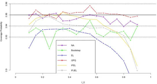
Figure 4.1 Coverage probabilities of the 95% confidence intervals for the Lorenz curve under Pareto distribution(n=100,200) . . . 17
Figure 4.2 Coverage probabilities of the 95% confidence intervals for the Lorenz curve under Pareto distribution(n=300,400) . . . 18
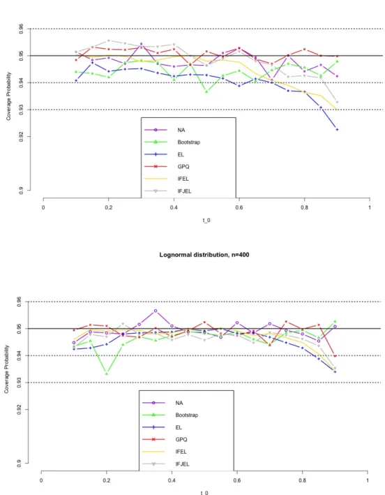
Figure 4.3 Coverage probabilities of the 95% confidence intervals for the Lorenz curve under Lognormal distribution(n=100,200) . . . 19
Figure 4.4 Coverage probabilities of the 95% confidence intervals for the Lorenz curve under Lognormal distribution(n=300,400) . . . 20
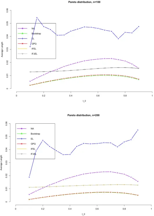
Figure 4.5 Average lengths of 95% confidence intervals for the Lorenz curve under Pareto distribution(n=100,200)(Note: IFEL almost overlaps IFJEL as their average lengths are very close, same for the GPQ and Boostrap.) 21
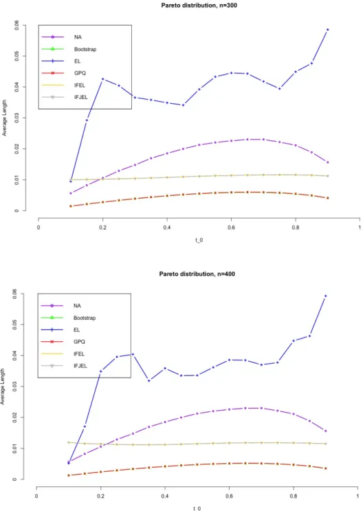
Figure 4.6 Average lengths of 95% confidence intervals for the Lorenz curve under Pareto distribution(n=300,400)(Note: IFEL almost overlaps IFJEL as their average lengths are very close, same for the GPQ and Boostrap.) 22
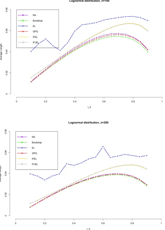
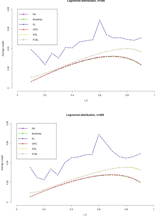
Figure 4.7 Average lengths of 95% confidence intervals for the Lorenz curve un-der Lognormal distribution(n=100,200)(Note: IFEL almost overlaps IFJEL as their average lengths are very close, same for the GPQ, Boostrap and NA.) . . . 23
Figure 4.8 Average lengths of 95% confidence intervals for the Lorenz curve un-der Lognormal distribution(n=300,400)(Note: IFEL almost overlaps IFJEL as their average lengths are very close, same for the GPQ, Boostrap and NA.) . . . 24
Figure 5.1 Histogram of Income Data . . . 26
Figure 5.2 Coverage probabilities of the 95% GCIs for the Lorenz curve under Pareto distribution(n=20) . . . 29
LIST OF ABBREVIATIONS
• ACI - Asymptotic Confidence Interval
• BCI - Bootstrap Confidence Interval
• CDF - Cumulative Distribution Function
• CI - Confidence Interval
• CvM - Cramer-von Mises
• EL - Empirical Likelihood
• GCI - Generalized Confidence Interval
• GPQ - Generalized Pivotal Quantity
• GSU - Georgia State University
• IFEL - Influence Function-based Empirical Likelihood
• IFJEL - Influence Function-based Jackknife Empirical Likelihood
• i.i.d. - independent identically distributed
• JEL - independent identically distributed
• KS - Kolmogorov-Smirnov
• MLE - Maximum Likelihood Estimator
• NA - Normal Approximation
• PEL - Profile Empirical Likelihood
CHAPTER 1
INTRODUCTION
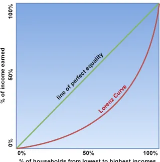
Much attention has been given to the rising income polarization in the U.S. and across the world, thus the estimation accuracy of the increasing income inequality is crucially important when government makes economic policy decisions. One widely used tool to measure the income distribution and income inequality is the Lorenz curve, which shows the percentage of the total income that the bottom (100 ∗t)% (t ∈ [0,1]) of households have. The Lorenz curve is illustrated in Figure 1, the line at the 45◦ angle shows perfect equality of income through all the households, while the Lorenz curve describes the inequality. The further away the Lorenz curve is from the diagonal, the more unequal is the income distribution.
Figure 1.1. Lorenz Curve
i.e., F(x) represents the proportion of the population whose income is less than or equal to
x. Assuming thatF(x) is differentiable, Gastwirth (1971)[14] provided a definition of Lorenz curve as below: η(t) = 1 µ Z ξt 0 xdF(x), t∈[0,1], (1.1) where µ = R∞
0 xdF(x) is the mean of F, and ξt = F
−1(t) = inf{x : F(x) ≥ t} is the t-th quantile ofF. For a fixedt∈[0,1], the Lorenz ordinateη(t) is the ratio of, the mean income of the lowest t-th fraction of households, and, the mean income of total households.
Lorenz curve has been primarily utilized in economics and social sciences. Atkinson (1970) [1] provided a theorem related to the social welfare function and the Lorenz curve, Doiron (1996) [9] used Lorenz dominance to analyze income and earning inequality. Be-sides economics, Lorenz curve is also widely used in other disciplines including medical and health research (Chang and Halfon 1997 [4]), industrial concentration (Smith 1947 [25]) and reliability (Gail and Gastwirth 1978 [13]).
Since income distribution F(x) is rarely known in practice, the Lorenz curve has to be estimated from the income data. LetX1, X2, . . . , Xn be a simple random sample drawn from the population X, the empirical estimate for η(t) is defined as
ˆ η(t) = 1 ˆ µ Z ξˆt 0 xdFˆn(x), t∈[0,1], (1.2)
where ˆFn(x) is the empirical distribution function of X1, X2, . . . , Xn, ˆµ is the sample mean, and ˆξt is the t-th sample quantile. One approach to make inferences on Lorenz curve is the normal approximation (NA) method (Beach and Davidson 1983 [2], Beach and Richmond 1985 [3], Cs¨org¨o and Zitikis 1996b [7]). However, the NA-based confidence intervals may have poor performances due to the skewness of the real income data. Bootstrap, introduced by Efron (1981[10], 1982a[11]), is another powerful statistical method to construct confidence intervals (Diciccio and Efron 1996[8]). There are still some limitations: 1) bootstrap method can be time consuming; 2) the sampling method used in generating bootstrap sample would also contribute to the sampling bias, according to Haukoos and Lewis (2005) [16].
Empirical likelihood (EL), introduced by Owen (1988) [20], has been shown to have di-verse advantages over the normal approximation and bootstrap method (Hall and La Scala 1990 [15]). For example, we can use EL method to construct a confidence interval without choosing an underlying distribution; the EL-based method is also able to construct confi-dence interval without variance estimation. As mentioned by Wood et al.(1996)[30], the EL ratio statistic, under mild conditions, converges in distribution to a chi-square distribu-tion. Thus, EL-based method may have advantages in developing statistical inferences with skewed data. EL has been widely used in many fields, such as survey sampling (Chen and Qin 1993 [5]), health care (Zhou et al. 2006[31]) and medical diagnostics (Qin and Zhou 2006 [23]). Recently, Qin, Yang and Belinga (2013) [22] developed a plug-in EL method to make inferences for the Lorenz curve. However, the limiting distribution of their EL ratio statistic is a scaled chi-square distribution, which requires heavy computation of the scale constant. Moreover the performances of their EL intervals are not stable due to the plug-in estimate of the scale constant. In order to alleviate the computational burden and obtain more con-sistent confidence intervals, we propose a new influence function-based empirical likelihood (IFEL) method to make inferences for the Lorenz curve. At the same time, the influence function-based Jackknife empirical likelihood (IFJEL) is implemented to be compared with IFEL method. Jackknife empirical likelihood (JEL) method was proposed by Jing, Yuan and Zhou (2009)[17] and the general idea of the JEL is to construct a jackknife pseudo-sample which is assumed to be asymptotically independent. Through simulation studies, we found that the proposed IFEL and IFJEL have good coverage probabilities in most cases except for those when t is large. Thus, it motivated us to propose the “exact” parametric inter-vals based on generalized pivotal quantities (GPQ), which has good performances in all the cases. In the GPQ method, we introduce two distributions which are the most commonly used parametric distributions for modeling income data: the Pareto distribution and the Lognormal distribution. The Pareto law for income distributions was developed and had been verified to hold universally by Pareto in 1897. The Pareto distribution fits the data fairly well toward the right tail of income and wealth distributions[29]. If we consider the
entire range of income, there is evidence that the income of 97%−99% of the population is distributed log-normally in economics studies[6]. Therefore, the fit may be better from the Lognormal distribution. Our GPQ-based approach is built on the concepts of generalized inferential procedures (Shafiei, Saboori and Doostparast, 2016 [24]) when the underlying income distribution is a Pareto distribution or a Lognormal distribution.
The rest of the thesis is organized as follows. In Chapter 2, we review the profile empirical likelihood (PEL) for Lorenz ordinate and propose the influence function-based empirical likelihood (IFEL) for Lorenz curve. Moreover, we implement the influence function-based Jackknife empirical likelihood (IFJEL) method. In Chapter 3, we briefly explain the methodology of generalized confidence interval (GCI) and the construction of confidence intervals for the Lorenz curve under Pareto and Lognormal distributions. In Chapter 4, we present various confidence intervals including normal approximation-based intervals and bootstrap-based intervals. Simulation studies are conducted to compare the performances of these proposed intervals. In Chapter 5, we use the income data from the Panel Study of Income Dynamics and median income data of twenty occupations in the U.S. in 1950 to illustrate the proposed intervals. In Chapter 6, there are some discussions and conclusions. The proof of the main theorem for the Lorenz curve is given in the Appendix.
CHAPTER 2
EMPIRICAL LIKELIHOOD-BASED METHODS
2.1 Influence Function-based Empirical Likelihood for the Lorenz Curve
Consider {X1, X2,· · · , Xn} as a simple random sample from the population of X with c.d.f. F. For a fixed t ∈ (0,1), the Lorenz ordinate η(t) must satisfies E[X(I(X ≤ ξt)−
η(t))] = 0. Thus, we can define the empirical likelihood for η(t) as follows:
˜ L1(η(t)) = sup p ( n Y i=1 pi : n X i=1 pi = 1, n X i=1 piDi(t) = 0 ) , (2.1)
where p = (p1, p2,· · · , pn) is a probability vector, Di(t) = Xi[I(Xi ≤ ξt)− η(t)], i = 1,2,· · · , n. Since the population quantile is unknown, we use the [nt]-th ordered value of
Xi’s to represent ξt, let’s say ˆξt = X[nt], we get the profile empirical likelihood (PEL) for
η(t): L1(η(t)) = sup p ( n Y i=1 pi : n X i=1 pi = 1, n X i=1 piDˆi(t) = 0 ) , (2.2) where ˆDi(t) =Xi[I(Xi ≤ξˆt)−η(t)], i= 1,· · · , n.
A unique maximum for p in (2.2) exists if η(t) is inside the convex hull of {X1[I(X1 ≤ ˆ
ξt)−η(t)], ..., Xn[I(Xn ≤ ξˆt)−η(t)]}. By Lagrange multiplier method, the supremum occurs at pi = n1
n
1 +ν(t) ˆDi(t) o−1
, i= 1,· · · , n, where ν(t) is the solution to
1 n n X i=1 ˆ Di(t) 1 +ν(t) ˆDi(t) = 0. (2.3) Note that Qn i=1pi, subject to Pn
n−n atp
i =n−1. So, the profile empirical likelihood ratio for η(t) can be defined as
R1(η(t)) = n Y i=1 (npi) = n Y i=1 {1 +ν(t) ˆDi(t)}−1 .
The corresponding profile empirical log-likelihood ratio for η(t) is:
l1(η(t)) = −2 logR1(η(t)) = 2 n X
i=1
log{1 +ν(t) ˆDi(t)}. (2.4)
The EL interval for η(t) is:
{η(t) :rl1(η(t))≤χ21,1−α}, (2.5) whereris the scale constant andr=s2
p(t)/s2d(t) withs2p(t) = R∞ 0 {x[I(x≤ξt)−η(t)]} 2dF(x), s2 d(t) = R∞ 0 [(x−ξt)I(x≤ξt)−xη(t)] 2dF(x)−(tξ t)2.
Based on the theories in Qin et al. (2013) [22], we can derive: 1 √ n Pn i=1Dˆi(t) = 1 √ n Pn i=1(Xi[I(X ≤ξˆt)−η(t)]) =√n{1 n Pn i=1[(Xi−ξt)I(Xi ≤ξt) +t0ξt−Xiη(t)]}+op(1) =√n{1 n Pn i=1g(Xi, η(t))}+op(1)
where g(Xi, η(t)) is called the influence function.
Next, we define the empirical likelihood based on influence function for η(t) as:
LIF(η(t)) = sup p ( n Y i=1 pi : n X i=1 pi = 1, n X i−1 piˆg(Xi, η(t)) = 0 ) . (2.6) where ˆg(Xi, η(t)) = (Xi−ξˆt)I(Xi ≤ξˆt) +tξˆt−Xiη(t).
And the EL ratio based on the estimated influence function can be defined as:
RIF(η(t)) = n Y i=1 (npi) = n Y i=1 {1 +νIF(t)ˆg(Xi, η(t))}−1, (2.7)
where νIF is the solution to: 1 n n X i=1 ˆ g(Xi, η(t)) 1 +νIF(t)ˆg(Xi, η(t)) = 0. (2.8)
The corresponding influence function-based empirical log-likelihood ratio for η(t) is:
lIF(η(t)) =−2logRIF(η(t)) = 2 n X
i=1
log{1 +νIF(t)ˆg(Xi, η(t))}, (2.9)
Then the following result gives the limiting distribution of the empirical likelihood based on influence function.
Theorem 1. If E(X2) < ∞ and η(t0) = E[XI(X ≤ξt0)]/E(X) for a given t = t0 ∈
(0,1), then the limiting distribution of lIF(η(t0)) is a standard chi-square distribution, i.e.,
lIF(η(t0))→χ21 as n→ ∞.
This theorem makes it much easier to construct confidence intervals for the Lorenz ordinates compared with the PEL method. Based on Theorem 1, a (1−α) level asymptotic confidence interval for Lorenz ordinateη(t) can be constructed as RIF ={η(t) :lIF(η(t))≤
χ21,1−α}.
2.2 Influence Function-based Jackknife Empirical Likelihood for the Lorenz Curve
Furthermore, we implement the influence function-based Jackknife empirical likelihood (IFJEL) method. Recall the influence function g(Xi, η(t0)) has been defined in Section 2.1. Let ˆ V−i = 1 n−1 n X j=1,j6=i ˆ g−i(Xj, η(t0)), i= 1,2,· · · , n, j = 1,2,· · · , n. (2.10)
where ˆg−i(Xj, η(t0)) = (Xj −ξˆt,−i)I(Xj ≤ ξˆt,−i) + tξˆt,−i −Xjη(t), ˆξt,−i is the ˆξt based on
ˆ Wi = n X j=1 ˆ g(Xj, η(t0))−(n−1) ˆV−i, i= 1,2,· · · , n, j = 1,2,· · ·, n. (2.11)
Here we use ˆWi to substitute ˆg(Xi, η(t0)) in (2.6) (2.7), (2.8) and (2.9), which gives the log influence function-based jackknife empirical likelihood ratio as
lIF J EL(η(t0)) = −2logRIF J EL(η(t0)) = 2 n X
i=1
log{1 +νIF J EL(t) ˆWi}, (2.12)
lIF J EL(η(t0)) can be proved to follow a standard chi-square distribution based on Jing, Yuan and Zhou’s paper (2009)[17]. Similar to the procedure in Section 2.1, we can construct the (1−α)% IFJEL confidence interval byRIF J EL={η(t) :lIF J EL(η(t))≤χ21,1−α}.
CHAPTER 3
GENERALIZED INFERENTIAL PROCEDURES FOR LORENZ CURVE UNDER PARETO AND LOGNORMAL DISTRIBUTIONS
Tsui and Weerahandi (1989)[26] introduced the concept of generalized p values and gen-eralized test variables, which are useful for developing hypothesis tests in situations involving nuisance parameters. Subsequently, the concept of a generalized pivotal quantity (GPQ) was introduced by Weerahandi (1993) [28]. In order to define a GPQ, letX be a random sample whose distribution depends on a parameter of interest θ, and a nuisance parameter δ. Let
x denote the observed value of X, then Q(X;x, θ, δ) is called a generalized pivotal quantity (GPQ) for θ, given the following two conditions:
(i) Given the observed value x, the distribution of Q(X;x, θ, δ) is free of any unknown parameter;
(ii) The observed value of Q(X;x, θ, δ) at X =x, i.e., Q(x;x, θ, δ), is equal to θ. From this definition, the percentiles of Q(X;x, θ, δ) are considered as the GCIs for θ. It’s easy to see that (Qα
2(X;x, θ, δ), Q1−
α
2(X;x, θ, δ)) is the equi-tail two-sided 100(1−α)% confidence interval for θ.
3.1 Lorenz Curve under Pareto Distribution
The Pareto distribution in the shape-scale form is defined as
F(x;β, λ) = P(X ≤x) = 1−(β
x)
1
λ, x≥β, (3.1)
whereλ andβ are the shape and the scale parameters, respectively. Moreover, Malik (1970) [18] derived distributions of the maximum likelihood estimators (MLEs) of the parameters in the Pareto distribution based on a random sample of sizen. Let X={X1,· · · , Xn}be a random sample from the Pareto distribution with the CDF (3.1). Then the MLEs of β and
λ are given by ˆ β= ˆβ(X) =X(1) and λˆ= ˆλ(X) = 1 n n X i=1 ln( Xi X(1) ), (3.2)
where X(1) denotes the first order statistic among X1,· · ·, Xn. Let
Z1 = 1 λln( ˆ β β) and Z2 = ˆ λ λ. (3.3)
Z1 and Z2 are independent random variables and 2nZ1 follows Chi-square distribution with 2 degrees of freedom, 2nZ2 follows Chi-square distribution with 2(n−1) degrees of freedom.
When the income distribution is a Pareto distribution, the Lorenz curve is
η(t;λ, β) = 1−(1−t)1−λ if 0< λ <1,0< t <1, 1 if 0< λ <1, t= 1. (3.4) Let Q∗λ = ˆ λ0 Z2 , (3.5)
where Z2 is defined by (3.3) and ˆλ0 denotes the observed value of ˆλ. It is easy to see that the distribution of Q∗λ is free of the unknown parameter λ, and 2nZ2 ∼ χ22(n−1). Moreover, the observed value of Q∗λ isλ. Therefore Qλ∗ is a GPQ for λ, and a GPQ for η(t;λ, β) is
Q0η(X;x, t, β) = 1−(1−t)1−Q∗λ if 0< Q∗ λ <1,0< t <1, 1 if 0< Q∗λ <1, t= 1. (3.6)
Since the CDF of Q0η(X;x, t, β) does not have a closed form, the following Monte Carlo method is needed to find GPQ-based CIs forη(t;λ, β).
We summarize the procedure in the following steps:
For a given random sample {x1, x2, ... , xn} from a pareto distribution, compute the value of ˆλ0.
1. Generate a random value of 2nZ2 from χ22(n−1), compute Q
∗
λ = 2nλˆ0
2nZ2, and then plug
Q∗λ in (3.6) to obtainQ0η.
2. Repeat step 1 for m (m is recommended to be 5000 or bigger) times, so we can get
m copies of Q0η.
3. Sort the m copies of Q0η in ascending order, and denote the ordered values as Q0η[1],
Q0η[2],· · ·, Q0η[m], where [a] means the greatest integer less than or equal toa.
Therefore the 100(1−α)% generalized confidence interval (GCI) forη(t;λ, β) is [Q0η[m∗
α/2], Q0η[m∗(1−α/2)]].
3.2 Lorenz Curve under Lognormal Distribution
A random variableX has a Lognormal distribution if its logarithmlog(X) has a normal distribution, i.e. Y =log(X)∼N(µ, σ2), and the MLE of µand σ2 is given by
ˆ µ= ¯Y = Pn i=1Yi n and σˆ 2 =S2 = Pn i=1(Yi−Y¯) 2 n−1 , (3.7) where Yi =log(Xi), ˆµand ˆσ2 are independent. And U2 = (n
−1)S2
σ2 ∼χ2n−1.
When the underlying distribution is a Lognormal distribution, the Lorenz curve is
η(t;µ, σ) =φ(φ−1(t)−σ) if 0< t <1, (3.8)
where φ denotes the probability density of the standard normal distribution. Let
Q∗σ2 =
s2(n−1)
U2 , (3.9) where s2 denotes the observed value of S2 = 1
n−1 Pn
i=1(Yi−Y¯)
2 and U2 = (n−1)S2
σ2 ∼ χ2n−1. The distribution of Q∗σ2 is free of unknown parameter σ2 and the observed value of Q∗σ2 is
σ2. Therefore, Q∗
σ2 is a GPQ for σ2 and the GPQ for η(t;µ, σ) is
Q∗η(X;x, t, σ) =φ(φ−1(t)−p
Similar to the case of Pareto distribution, we have the following steps to find GPQ-based CIs for η(t;µ, σ).
For a given random sample {x1, x2, ... , xn} from a Lognormal distribution, compute the value of s2.
1. Generate a random value of U2 from χ2
n−1, compute Q∗σ2 =
s2(n−1)
U2 , and then plug
Q∗σ2 in (3.10) to obtain Q∗η.
2. Repeat step 1 for m times, so we can get m copies {Q∗η,1, Qη,∗2,· · · , Q∗η,m} of Q∗η. 3. Sort the m copies of Q∗η in ascending order, and denote the ordered values as Q∗η[1],
Q∗η[2],· · ·, Q∗η[m].
The 100(1 − α)% generalized confidence interval (GCI) for η(t;µ, σ) is [Q∗η[m ∗
CHAPTER 4
SIMULATION STUDIES
In this part, intensive simulation studies are conducted to evaluate finite sample per-formance of the proposed methods.
4.1 Influence Function-based Empirical Likelihood Intervals
Based on Theorem 1, the 100(1−α)% confidence interval is defined as RIF = {η(t) :
lIF(η(t))≤ χ21,1−α}. By the influence function-based empirical likelihood (IFEL) approach, the coverage probability is calculated using the following procedures:
1. Generate {x1, x2,· · · , xn}from an underlying distribution.
2. Calculate η(t0) for fixed t0, solve equation (2.8) for νIF(t0) and get the value of log-likelihood lIF(η(t0)) =−2logRIF(η(t0)) = 2Pin=1log{1 +νIF(t)ˆg(Xi, η(t0))}.
3. Set the initial value of (η(t), νIF(t)) as (η(t0)−0.1,0). Then obtain the solution η1 for η(t) by solving the nonlinear equations (2.8) and
lIF(η(t))−χ21,1−α = 0 (4.1)
where lIF(η(t)) = 2Pni=1log{1 +νIF(t)ˆg(Xi, η(t))}. Set (η(t0) + 0.1,0) as the initial value of (η(t), νIF(t)) and solve the nonlinear equations again, get solution η2. The interval length is calculated by η2−η1.
4. Repeat 1-3 for B (a large number, e.g. B=5000) times, then calculate the coverage probability of the IFEL interval:
1 B B X b=1 I(lIF,b(η(t0))≤χ21,1−α), (4.2)
and the average length of the confidence interval is 1 B B X b=1 (η2,b−η1,b), (4.3)
wherelIF,b(η(t0)),η1,b and η2,b are the values oflIF(η(t0)),η1 andη2 based onb-th simulated sample, respectively.
Similarly, we can calculate the coverage probability and average length of IFJEL interval.
4.2 Asymptotic Confidence Intervals
One of the most popular methods to construct a confidence interval for an unknown parameter is the normal approximation. Since the MLE’s (ˆλ,βˆ) of Lorenz curve under Pareto distributions is invariant. Under the proper regularity assumptions, as n→ ∞, we have the following asymptotical result,
√
n(η(t; ˆλ,βˆ)−η(t;λ, β))−→d N(0,(Oη(t;λ, β))|I(Θ)−1(Oη(t;λ, β))), as n→ ∞, (4.4)
where ˆΘ = (ˆλ,βˆ)| has an asymptotic bivariate normal distribution with mean Θ = (λ, β)| and the covariance matrix determined by the Fisher information matrixI(Θ), Oηis the first derivative ofη(t;λ, β).
There is a consistent estimator for Fisher information matrix I(Θ), which is proposed by Meilijson (1989) [19]. Letli(xi,Θ) represent the single observation log-likelihood function and
si(xi,Θ) =
∂li(xi,Θ)
∂Θ (4.5)
be the score function. Then the empirical Fisher information matrixH(x,Θ) can be defined as, H(x,Θ) = 1 n n X i=1 si(xi,Θ)si(xi,Θ)|− 1 n2S(x,Θ)S(x,Θ) | (4.6) whereS(x,Θ) =Pn
to be estimated by ˆIn(Θ) = nH(x,Θ). Therefore, an asymptotic 100(1ˆ −α)% confidence interval (ACI) forη(t;λ, β) is
ACI = (η(t; ˆλ,βˆ)−z1−α/2σ, ηˆ (t; ˆλ,βˆ) +z1−α/2σˆ) (4.7)
where ˆσ = ((Oη(t; ˆλ,βˆ))|(nH(x,Θ))ˆ −1(Oη(t; ˆλ,βˆ)))1/2, Oη(t; ˆλ,βˆ) is the matrix gradient of
η(t;λ, β) at Θ = ˆΘ and zα is the α-th quantile of the standard normal distribution. When the underlying income distribution is a Lognormal distribution, we use the same way to find the ACI for η(t;µ, σ).
4.3 Bootstrap Confidence Intervals
The empirical bootstrap is a statistical technique popularized by Efron (1993)[12]. The key idea is to perform computations on the data itself to estimate the specific statistics from the same data. The bootstrap setup is as follows:
1. Generate {x1, x2,· · · , xn} from a Pareto distribution with parameters λ and β, compute the MLE’s ˆλ and ˆβ.
2. Generate bootstrap samplex∗ ={x∗1, x∗2,· · · , x∗n}from{x1, x2,· · · , xn}, compute the bootstrap copies ˆλ∗ and ˆβ∗ of ˆλ and ˆβ based on the bootstrap sample, then plug them in the Lorenz curve ˆη∗ =η∗(t,λˆ∗,βˆ∗).
3. Repeat steps 1-2 for B (a large number, e.g. B=5000) times and get B bootstrap copies of ˆη∗. Let ˆη1∗,ηˆ2∗,· · · ,ηˆ∗Bdenote the bootstrap copies in ascending order, the (1−α)-th percentile bootstrap confidence interval (BCI) for Lorenz ordinate η(t) is given by
BCI = (ˆη∗[Bα/2],ηˆ[∗B(1−α/2)]) (4.8)
where ˆη[∗Bα] is the [Bα]-th value in the ordered list of the B replications of ˆη∗.
When the underlying distribution is a Lognormal distribution, we use the same algo-rithm to construct the confidence interval for Lorenz curve.
4.4 Simulation results
When generating samples, we should notice that most income distributions are positively skewed, so the choice of underlying distributionF should be a positively skewed distribution. In this part, we choose Pareto distribution with the shape parameter λ1 = 151 and the scale parameter β= 0.9, and Lognormal distribution with meanµ= 0.05 and standard deviation
σ = 0.5. The sample size n is chosen to be 100, 200, 300 and 400. B andm are set as 5000. Let t0 = 0.1 + 0.05k, k = 0,1,· · ·,16, we calculate the coverage probabilities and average interval lengths of 95% level confidence intervals for η(t0).
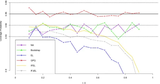
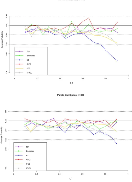
Figures 4.1− 4.8 show the simulation results. First, we observe that the coverage probabilities of the GCIs are very close to the nominal level in all the cases, and GCIs perform much better than ACIs and BCIs when sample size is small. IFEL and IFJEL also have good performances except for cases when t0 falls in the upper tail of Lorenz curve, and they both outperform EL with better coverage probabilities. As sample size increases, the coverage probabilities of IFEL and IFJEL confidence intervals are in better agreement with the nominal level. Second, when we look at the average lengths of all the confidence intervals, GCIs and BCIs have similar average lengths and they are the shortest among all the confidence intervals. We also observe that IFEL and IFJEL confidence intervals have comparable average lengths, while EL confidence intervals has the longest average lengths. Overall, we recommend the GCI for the Lorenz curve when underlying distribution is a Pareto distribution or a Lognormal distribution, and recommend the IFEL confidence interval and IFJEL confidence interval for Lorenz curve when underlying distribution is unknown.
Figure 4.1. Coverage probabilities of the 95% confidence intervals for the Lorenz curve under Pareto distribution(n=100,200)
Figure 4.2. Coverage probabilities of the 95% confidence intervals for the Lorenz curve under Pareto distribution(n=300,400)
Figure 4.3. Coverage probabilities of the 95% confidence intervals for the Lorenz curve under Lognormal distribution(n=100,200)
Figure 4.4. Coverage probabilities of the 95% confidence intervals for the Lorenz curve under Lognormal distribution(n=300,400)
Figure 4.5. Average lengths of 95% confidence intervals for the Lorenz curve under Pareto distribution(n=100,200)(Note: IFEL almost overlaps IFJEL as their average lengths are very close, same for the GPQ and Boostrap.)
Figure 4.6. Average lengths of 95% confidence intervals for the Lorenz curve under Pareto distribution(n=300,400)(Note: IFEL almost overlaps IFJEL as their average lengths are very close, same for the GPQ and Boostrap.)
Figure 4.7. Average lengths of 95% confidence intervals for the Lorenz curve under Lognormal distribution(n=100,200)(Note: IFEL almost overlaps IFJEL as their average lengths are very close, same for the GPQ, Boostrap and NA.)
Figure 4.8. Average lengths of 95% confidence intervals for the Lorenz curve under Lognormal distribution(n=300,400)(Note: IFEL almost overlaps IFJEL as their average lengths are very close, same for the GPQ, Boostrap and NA.)
CHAPTER 5
REAL DATA EXAMPLES
5.1 Public Income Data from the Panel Study of Income Dynamics
In this section, we apply the proposed methods to make inferences for Lorenz curve with a real income dataset. Income inequality is a significant economic problem all over the world and the United States have the highest rising of income inequality among most developed countries (Weeks 2007 [27]). By constructing confidence intervals for Lorenz ordinates at different t, we can discuss how the income inequality is in the United States and have a general view of the inequality.
This income dataset is obtained from the database - The Panel Study of Income Dynam-ics (PSID) - from the University of Michigan (PSID 2017 [21]). It is part of the 2015 PSID Main Family Data, and it contains three variables: ER60001 - Release Number, ER60002 - 2015 Family Interview (ID) Number and ER65349 - Total Family Income-2014. The in-come reported here was collected in 2015 for tax year 2014. Please note that this variable can contain negative values. Negative value indicates a net loss, which in waves prior to 1994. These losses occur as a result of business or farm loss. Positive values mean actual income amounts and zero means there is no family income in 2014. There are in total 9048 households in this dataset.
A brief summary of this income data is shown in Table 5.1:
Table 5.1. Summary of 2015 PSID Family Data - Income
Min. 1st Qu. Median Mean 3rd Qu. Max.
-22000 24000 49310 69540 90210 5250000
Figure 5.1. Histogram of Income Data
Here we utilize the Pareto distribution and Lognormal distribution to fit this income data. In order to test the goodness-of-fit, the popular goodness-of-fit index named Kolmogorov-Smirnov (K-S) statistic is used. We consider the null hypothesisH0 :X ∼P areto(β, λ) and
H0 :X ∼Lognormal(µ, σ2), the p-values for Pareto distribution and Lognormal distribution are both far less than 0.05. These p-values indicate that the income data does not follow a Pareto distribution nor a Lognormal distribution. So we can only use nonparametric methods, i.e. IFEL, IFJEL and EL methods to construct confidence intervals for Lorenz curve.
The non-parametric estimates for the Lorenz ordinates with their 95% confidence inter-vals are presented in Table 5.2. We can see that IFEL and IFJEL intervals are very similar in most cases. Based on our simulation results, we suggest to use IFEL and IFJEL intervals. For example, when t = 0.9, the 95% IFEL confidence interval for Lorenz curve is (0.6456; 0.6654), it means the ratio of the mean income of the lowest 90% households and the mean income of total households is greater than 0.6456, but smaller than 0.6654.
Table 5.2. 95% level confidence intervals for Lorenz ordinates IFEL IFJEL EL
t Confidence interval Confidence interval Confidence interval 0.10 (0.0032,0.0110) (0.0002,0.0080) (0.0043,0.0116) 0.20 (0.0270,0.0306) (0.0240,0.0276) (0.0339,0.0392) 0.30 (0.0588,0.0652) (0.0558,0.0622) (0.0739,0.0850) 0.40 (0.1065,0.1146) (0.1035,0.1116) (0.1334,0.1439) 0.50 (0.1640,0.1776) (0.1610,0.1746) (0.2080,0.2194) 0.60 (0.2458,0.2582) (0.2428,0.2552) (0.2958,0.3147) 0.70 (0.3477,0.3597) (0.3447,0.3567) (0.4186,0.4313) 0.80 (0.4750,0.4900) (0.4720,0.4870) (0.5551,0.5705) 0.90 (0.6456,0.6654) (0.6426,0.6624) (0.7207,0.7391)
5.2 Median Income Data of Twenty Occupations in the U. S. in 1950
The second data set is about the median income of the twenty occupations in the United States Census of Population, 1950, Occupational Characteristics (Special Report,P-E No. 1B)(Shafiei, Saboori and Doostparast, 2016 [24]). The data set is presented in Table 5.3. The p-value of K-S test for Pareto distribution with parameters β and λ is 0.9905, the p-value of K-S test for Lognormal distribution with parameters µ and σ2 is far less than 0.05. These p-values suggest that the median income data follows a Pareto distribution, so we use the Pareto distribution to model the median income data.
We recommend to use GCI for Lorenz curve as it has best performances in our simulation studies. Figure 5.2 shows the coverage probabilities of the 95% GCIs for the Lorenz curve under Pareto distribution when sample size is 20, which is the same size as the median income data. We can observe that the coverage probabilities are all very close to the nominal level 0.95. Table 5.4 displays various 95% level confidence intervals for Lorenz curve. For example, when t = 0.1, the 95% GCI for Lorenz curve is (0.0485, 0.0799), it means the ratio of the mean income of the lowest 10% occupations and the mean income of total occupations is greater than 0.0485, but smaller than 0.0799.
Table 5.3. Median income (by 1949 in dollars) of 20 occupations in the United States.
Occupation Income Occupation Income Accountants and auditors 3977 Mail-carriers 3480 Architects 5509 Plumbers and pipe fitters 3353 Authors, editors, and reporters 4303 Motormen, street, subway, and
ele-vated rai1way
3424
Chemists 4091 Teachers (n.e.c.) 3456 Dentists 6448 Insurance agents and brokers 3771 Engineers, civil 4590 Electricians 3447 Lawyers and judges 6284 Locomotive engineers 4648 Physicians and surgeons 8302 Machinists and job setters, metal 3303 College presidents, professors, and
in-structors (n.e.c.)
4366 Managers, officials, and proprietors (n.e.c.) - self-employed - wholesale and retail trade
3806
Managers, officials, and proprietors (n.e.c.) - self-employed - manufactur-ing
4700
Figure 5.2. Coverage probabilities of the 95% GCIs for the Lorenz curve under Pareto distribution(n=20)
Table 5.4. Length of 95% CI for median income data of 20 occupations in the United States
t Method Confidence interval t Method Confidence interval
0.1 GCI (0.0485,0.0799) 0.7 GCI (0.4360,0.6145) ACI (0.0566,0.0864) ACI (0.4930,0.6500) BCI (0.0589,0.0837) BCI (0.5019,0.6319) IFEL (0.0620,0.0800) IFEL (0.5364,0.6330) IFJEL (0.0499,0.0499) IFJEL (0.5376,0.6334) EL (0.0319,0.0397) EL (0.5458,0.6419) 0.3 GCI (0.1604,0.2458) 0.9 GCI (0.6669,0.8381) ACI (0.1798,0.2642) ACI (0.7330,0.8715) BCI (0.1852,0.2572) BCI (0.7387,0.8530) IFEL (0.1979,0.2518) IFEL (0.7915,0.8563) IFJEL (0.1978,0.2524) IFJEL (0.7943,0.8587) EL (0.1811,0.1836) EL (0.8000,0.8634) 0.5 GCI (0.2831,0.4218) ACI (0.3214,0.4508) BCI (0.3298,0.4375) IFEL (0.3486,0.4303) IFJEL (0.3374,0.3818) EL (0.3498,0.3569)
CHAPTER 6
CONCLUSIONS
In this thesis, an empirical likelihood method based on influence function is proposed and used to construct confidence intervals for the Lorenz ordinates. The Jackknife empirical likelihood method based on influence function is carried out. At the same time, we develop the generalized confidence intervals for Lorenz ordinates under Pareto and Lognormal dis-tributions. Since Pareto and the lognormal distributions play a central role as probabilistic models for the distributions of various phenomena in different fields, the confidence intervals derived in this thesis should be of practical interest.
Simulation results show good coverage probabilities of influence function-based empiri-cal likelihood confidence intervals and influence function-based Jackknife empiriempiri-cal likelihood confidence intervals in the lower tails when the sample size is large. Moreover, the coverage probabilities of the generalized confidence intervals are in good agreement with the nominal level for all the cases considered. They have pretty good performances even for the small samples, compared with the bootstrap confidence intervals and asymptotic confidence inter-vals. The real data examples show the confidence intervals for Lorenz ordinates at different t’s, which gives us a general view of the income inequality and how severe it is in the United States. It also gives us an idea when to use our proposed methods. In sum, if the underlying income distribution is a Pareto distribution or a Lognormal distribution, generalized confi-dence interval could give us a better way to make inferences on Lorenz curve. If it is hard to know the underlying distribution or to fit a Pareto or a Lognormal distribution to the data, influence function-based empirical likelihood and influence function-based Jackknife empirical likelihood methods will be very useful in constructing confidence intervals for the Lorenz Curve.
REFERENCES
[1] A. B. Atkinson. On the measurement of inequality. Journal of Economic Theory, 2:244–263, 1970.
[2] C. M. Beach and R. Davidson. Distribution-free statistical inference with lorenz curves and income shares. Review of Economic Studies, 50:723–735, 1983.
[3] C. M. Beach and J. Richmond. Joint confidence intervals for income shares and lorenz curves. International Economic Review, 26:439–450, 1985.
[4] R. Chang and N. Halfon. Graphical distribution of pediatricians in the united states: An analysis of the fifty states and washington, dc. Pediatrics, 100:172–179, 1997.
[5] J. H. Chen and J. Qin. Empirical likelihood estimation for finite populations and the effective usage of auxiliary information. Biometrika, 80:107–116, 1993.
[6] F. Clementi and M. Gallegati. Pareto’s law of income distribution: Evidence for ger-many, the united kingdom, and the united states. In Chatterjee A., Yarlagadda S., and Chakrabarti B.K., editors,Econophysics of Wealth Distributions. Springer, Milano, 2005.
[7] M. Cs¨org¨o and R. Zitikis. Strassens lil for the lorenz curve. Journal of Multivariate
Analysis, 59:1–12, 1996.
[8] J. T. DiCiccio and B. Efron. Bootstrap confidence intervals. Statistical Science, 11(3):189–228, 1996.
[9] D. J. Doiron and G. F. Barrett. Inequality in male and female earnings: the roles of hours and earnings. Review of Economics and Statistics, 78:410–420, 1996.
[10] B. Efron. Nonparametric standard errors and confidence intervals (with discussion).
[11] B. Efron. The Jackknife, the Boostrap, and Other Resampling Plans. Philadelphia, Pa.: Society for Industrial and Applied Mathematics, 1982.
[12] B. Efron. An Introduction to the Bootstrap. Chapman: Hall/CRC, 1993.
[13] M. H. Gail and J. L. Gastwirth. A scale-free goodness-of-fit test for the exponential distribution based on the lorenz curve. Journal of the American Statistical Association, 73:229–243, 1978.
[14] J. L. Gastwirth. A general definition of lorenz curve. Econometrica, 39:1037–1039, 1971.
[15] P. Hall and B. La Scala. Methodology and algorithms of empirical likelihood.
Interna-tional Statistical Review, 58:109–127, 1977.
[16] J. S. Haukoos and R. J. Lewis. Advanced statistics: bootstrapping confidence intervals for statistics with ’difficult’ distributions. Academic Emergency Medicine, 12:360–365, 2005.
[17] B. Jing, J. Yuan, and W. Zhou. Jackknife empirical likelihood. Journal of the American
Statistical Association, 104:1224–1232, 2009.
[18] H. J. Malik. Estimation of the parameters of the pareto distribution. Metrika, 16:126– 132, 1970.
[19] I. Meilijson. A fast improvement to the em algorithm on its own terms. Journal of the
Royal Statistical Society, Series B, 51:127–138, 1970.
[20] A. Owen. Empirical likelihood ratio confidence intervals for single functional.
Biometrika, 75:237–249, 1988.
[21] PSID. Panel Study of Income Dynamics, public use dataset. Produced and distributed by the Institute for Social Research, University of Michigan, Ann Arbor, MI. 2017.
[22] G. S. Qin, B. Y. Yang, and N. E. Belohnga-Hill. Empirical likelihood-based inferences for the lorenz curve. Annals of the Institute of Statistical Mathematics, 65:1–21, 2013.
[23] G. S. Qin and X. H. Zhou. Empirical likelihood inference for the area under the roc curve. Biometrics, 62:613–622, 2006.
[24] S. Shafiei, H. Saboori, and M. Doostparast. Generalized inferential procedures for gen-eralized lorenz curves under the pareto distribution. Journal of Statistical Computation
and Simulation, 87:267–279, 2016.
[25] G.C. Smith JR. Lorenz curve analysis of industrial decentralization. Journal of the
American Statistical Association, 42:591–596, 1947.
[26] K. W. Tsui and S. Weerahandi. Generalized p-values in significance testing of hypotheses in the presence of nuisance parameters. Journal of the American Statistical Association, 84:602–607, 1989.
[27] J. Weeks. Inequality trends in some developed oecd countries. United Nations DESA
Woking Paper, 6:1–14, 2007.
[28] S. Weerahandi. Generalized confidence intervals. Journal of the American Statistical
Association, 88:899–905, 1993.
[29] Wikipedia. Pareto principle, 2018. [Online at https://en.wikipedia.org/wiki/ Pareto_principle; accessed 20-Feb-2018].
[30] A.T.A. Wood, K.A. Do, and N.M. Broom. Sequential linearization of empirical likeli-hood constraints with application to u-statistics. Journal of Computational and
Graph-ical Statistics, 5(4):365–385, 1996.
[31] X. H. Zhou, G. S. Qin, H. Z. Lin, and G. Li. Inferences in censored cost regression models with empirical likelihood. Statistica Sinica, 16:1213–1232, 2006.
Appendix A
PROOF OF THEOREMS
Lemma 1. Under the conditions in Theorem 1, we have
1 n n X i=1 (ˆg(Xi, η(t0))−g(Xi, η(t0)))2 =op(1) Proof of Lemma 1.
For a given t0, let g(Xi, η(t0)) = (Xi−ξt0)I(Xi ≤ ξt0) +t0ξt0 −Xiη(t0). The difference between ˆg(Xi, η(t0)) andg(Xi, η(t0)) can be expressed as
ˆ
g(Xi, η(t0))−g(Xi, η(t0)) =Ai +Bi
where
Ai = (Xi−ξˆt0)I(Xi ≤ξˆt0)−(Xi−ξt0)I(Xi ≤ξt0)
Bi =t0( ˆξt0 −ξt0)
Applying the inequality (a+b)2 ≤2(a2+b2), we obtain that 1 n n X i=1 (ˆg(Xi, η(t0))−g(Xi, η(t0)))2 = 1 n n X i=1 (Ai+Bi)2 ≤ 2 n n X i=1 A2i + 2 n n X i=1 Bi2
Therefore, we only need to prove that the sample means of A2
i and Bi2 converge to zero in probability. The proofs will be presented in (A) and (B) below.
(A) 1nPn i=1A
2
1 n n X i=1 A2i = 1 n n X i=1 [(Xi−ξˆt0)I(Xi ≤ξˆt0)−(Xi−ξt0)I(Xi ≤ξt0)] 2 = 1 n n X i=1 [Xi2I(Xi ≤ξˆt0)(I(Xi ≤ξˆt0)−I(Xi ≤ξt0))−2Xiξˆt0I(Xi ≤ξˆt0)(I(Xi ≤ξˆt0) −I(Xi ≤ξt0)) + ˆξt0I 2(X i ≤ξˆt0)( ˆξt0I(Xi ≤ξˆt0)−ξt0I(Xi ≤ξt0) + 2Xiξt0I(Xi ≤ξt0)(I(Xi ≤ξˆt0)−I(Xi ≤ξt0))−X 2 iI(Xi ≤ξt0)(I(Xi ≤ξˆt0) −I(Xi ≤ξt0))−ξt0I(Xi ≤ξt0)( ˆξt0I(Xi ≤ξˆt0)−ξt0I(Xi ≤ξt0))]
By the strong consistency of the sample quantile ˆξt0, we obtain that |I(Xi ≤ ξˆt0)−
I(Xi ≤ ξt0)| p − → 0 , |ξˆt0I(Xi ≤ ξˆt0)− ξt0I(Xi ≤ ξt0)| p − → 0 , for i = 1,2,· · ·, n . From 1 n Pn
i=1|Xi|2 →E(X2)<∞ a.s., it follows that 1 n n X i=1 A2i =op(1) (B) 1nPn i=1Bi2 =op(1)
It’s obvious that|ξˆt0 −ξt0| p − →0, thus n1 Pn i=1B 2 i =op(1). Lemma 2. (i) maxi|gˆ(Xi, η(t0))|=op( √ n). (ii) n1Pn i=1ˆg 2(X i, η(t0)) =σ2+op(1). (iii) √1 n Pn i=1gˆ(Xi, η(t0)) d − →N(0, σ2). Proof of Lemma 2.
(i) Since g(Xi, η(t0)) are i.i.d. random variables with zero mean and finite variance σ2, maxi|g(Xi, η(t0))|=op( √ n). We obtain that max i |gˆ(Xi, η(t0))| ≤maxi |gˆ(Xi, η(t0))−g(Xi, η(t0))|+ maxi |g(Xi, η(t0))|=op( √ n)
(ii) Similar to proof of Lemma 1, we can prove that 1 n n X i=1 g(Xi, η(t0))(ˆg(Xi, η(t0))−g(Xi, η(t0))) =op(1). (A.1)
Then from Lemma 1, (A.1), (A.2) and n1Pn
i=1g2(Xi, η(t0)) =σ2, we have that 1 n n X i=1 ˆ g2(Xi, η(t0)) = 1 n n X i=1 (ˆg(Xi, η(t0))−g(Xi, η(t0)))2+ 1 n n X i=1 g(Xi, η(t0))2 + 2 n n X i=1 g(Xi, η(t0))(ˆg(Xi, η(t0))−g(Xi, η(t0))) =σ2+op(1). (A.2)
Lemma 2(ii) is proved.
(iii) Similar to proof of Lemma 1, we can obtain that
1 √ n n X i=1 (ˆg(Xi, η(t0))−g(Xi, η(t0))) =op(1). (A.3) Then we have 1 √ n n X i=1 ˆ g(Xi, η(t0)) = 1 √ n n X i=1 (ˆg(Xi, η(t0))−g(Xi, η(t0))) + 1 √ n n X i=1 g(Xi, η(t0)) = √1 n n X i=1 g(Xi, η(t0)) +op(1) (A.4) From √1 n Pn i=1g(Xi, η(t0)) d −
→N(0, σ2), Lemma 2(iii) is proved. Proof of Theorem 1.
Using Lemma 2 and Lemmas in Owen (1990), we have |νIF| = Op(n− 1
2). Applying Taylor expansion to (2.9), we can obtain
lIF(η(t0)) = 2 n X i=1 log{1 +νIF(t0)ˆg(Xi, η(t0))} = 2 n X i=1 (νIF(t0)ˆg(Xi, η(t0))−12(νIF(t0)ˆg(Xi, η(t0))2) +r1n
with|r1n| ≤CPni=1|νIF(t0)ˆg(Xi, η(t0))|3 ≤C|νIF(t0)|3maxi|gˆ(Xi, η(t0))|Pni=1gˆ2(Xi, η(t0)) = op(1). From (2.8), n X i=1 ˆ g(Xi, η(t0)) 1 +νIF(t0)ˆg(Xi, η(t0)) = n X i=1 ˆ g(Xi, η(t0))[1−νIF(t0)ˆg(Xi, η(t0)) + (νIF(t0)ˆg(Xi, η(t0)))2 1 +νIF(t0)ˆg(Xi, η(t0)) ] = n X i=1 ˆ g(Xi, η(t0))−νIF(t0) n X i=1 ˆ g2(Xi, η(t0))+ n X i=1 ˆ g(Xi, η(t0))(νIF(t0)ˆg(Xi, η(t0)))2 1 +νIF(t0)ˆg(Xi, η(t0)) = 0, it follows thatνIF(t0) = Pn i=1ˆg(Xi,η(t0)) Pn i=1ˆg2(Xi,η(t0))+op(n −1
2). Further, we have thatPn
i=1νIF(t0)ˆg(Xi, η(t0)) = Pn
i=1(νIF(t0)ˆg(Xi, η(t0)))2+op(1).
Therefore, by Lemma 1, we obtain that
lIF(η(t0)) = n X i=1 (νIF(t0)ˆg(Xi, η(t0)))2 +op(1) = ( 1 √ n Pn i=1gˆ(Xi, η(t0)))2 1 n Pn i=1gˆ2(Xi, η(t0)) +op(1) =χ21+op(1).