data and meta-classifier selection in multiple classifier system. In López-Ibáñez, M. (ed.) Proceedings of the
2019
Genetic and
evolutionary computation conference (GECCO '19), 13-17 July 2019, Prague, Czech Republic. New
York: ACM [online], pages 39-46.
Available from:
https://doi.org/10.1145/3321707.3321770
Simultaneous meta-data and meta-classifier
selection in multiple classifier system.
NGUYEN, T.T., LUONG, A.V., NGUYEN, T.M.V., HA, T.S., LIEW, A.W.-C.,
MCCALL, J.
2019
This document was downloaded from
https://openair.rgu.ac.uk
© ACM, 2019. This is the author's version of the work. It is posted here by permission of ACM for your personal use.
Not for redistribution. The definitive version was published in Proceedings of the 2019 Genetic and Evolutionary
Multiple Classifier System
Tien Thanh Nguyen
School of Computing Science and Digital Media
Robert Gordon University, Aberdeen United Kingdom
Anh Vu Luong
School of Information and Communication Technology Griffith University, Gold Coast
Australia
Thi Minh Van Nguyen
Department of Planning and Investment
Ba Ria Vung Tau, Vietnam [email protected]
Trong Sy Ha
School of Applied Mathematics and Informatics
Hanoi University of Science and Technology, Hanoi, Vietnam
Alan Wee-Chung Liew
School of Information and Communication Technology Griffith University, Gold Coast
Australia [email protected]
John McCall
School of Computing Science and Digital Media
Robert Gordon University, Aberdeen United Kingdom
ABSTRACT
Inensemblesystems,thepredictionsofbaseclassifiersare aggre-gatedbyacombiningalgorithm(meta-classifier)toachievebetter classificationaccuracythanusingasingleclassifier.Experiments showthat theperformanceofensemblessignificantlydepends onthechoiceofmeta-classifier.Normally,theclassifierselection methodappliedtoanensembleusuallyremovesallthepredictions ofaclassifierifthisclassifierisnotselectedinthefinalensemble. Herewepresentanideatoonlyremoveasubsetofeach clas-sifier’spredictiontherebyintroducingasimultaneousmeta-data andmeta-classifierselectionmethodforensemblesystems.Our approachusesCross Validationonthetrainingsettogenerate meta-dataasthepredictionsofbaseclassifiers.WethenuseAnt ColonyOptimizationtosearchfortheoptimalsubsetofmeta-data andmeta-classifierforthedata.Byconsideringeachcolumnof meta-data,weconstructtheconfigurationincludingasubsetof thesecolumnsandameta-classifier.Specifically,thecolumnsare selectedaccordingtotheircorrespondingpheromones,andthe meta-classifierischosenatrandom.Theclassificationaccuracy ofeachconfigurationiscomputedbasedonCrossValidationon meta-data.ExperimentsonUCIdatasetsshowtheadvantageof pro-posedmethodcomparedtoseveralclassifierandfeatureselection methodsforensemblesystems.
CCS
CONCEPTS
•Mathematics of computing→Evolutionary algorithms; • Com-puting methodologies→Ensemble methods;
KEYWORDS
Ensemblemethod,multipleclassifiers,classifierfusion,combining classifiers,ensembleselection,classifierselection,featureselection, AntColonyOptimization
1
INTRODUCTION
LearningfromtheEnsembleofClassifiers(EoC)toachievehigher classificationaccuracythanusingasingleclassifierisoneofthe mostpopulartopicsinmachinelearningresearch.Aseachclassifier isahypothesisabouttherelationshipbetweenthefeaturesofan observationanditsclasslabel,bycombiningseveralbase classi-fiersinanensemble,wecanobtainbetterapproximationforthis relationship,therebyenhancetheperformanceoftheclassification system[17,19].
Therearethreephasestobeconsideredinanensembledesign, namelygeneration,selection,andintegration.Inthegeneration phase,thelearningalgorithm(s)learnonthetrainingset(s)to ob-tainthebaseclassifiers.Intheselectionphase,asingleclassifieror asubsetofthebestclassifiersisselectedtoclassifythetestsample. Inthelastphase,thedecisionsmadebytheselectedEoCare com-binedtoobtainthefinalprediction[3,7].Homogeneousensemble methodslikeBagging[2],andRandomSubspace[1]focusonthe generationphaseinwhichtheyconcentrateonthegenerationof newtrainingschemesfromtheoriginaltrainingset.Meanwhile, heterogeneousensemblemethodsfocusoncombiningalgorithms whichoperateontheoutputsofthebaseclassifiers(called meta-dataorLevel1data)[17–20].Thecombiningalgorithmisalsocalled ameta-classifier.
Inthisstudy,wefocusontheselectionphaseintheensemble designbyproposingasimultaneousmeta-dataandmeta-classifier
selection method for heterogeneous ensemble systems. In an en-semble system, there usually exists a subset of EoC that makes the ensemble perform better than using the entire set of base classi-fiers. However, as pruning a classifier’s output is more general then pruning the classifier itself, we are motivated to expect meta-data selection to result in better performance. Moreover, in a heteroge-neous ensemble system, the performance of the ensemble system depends on the performance of the meta-classifier [26]. Therefore, by doing meta-data and meta-classifier selection simultaneously, we could obtain a higher performance ensemble than other existing selection-based ensemble systems.
This paper introduces a method to simultaneously select the sub-set of meta-data and the meta-classifier to obtain a high-performance ensemble system. We first generate the base classifiers and then the meta-data from the training observations. Having the meta-data and the given set of meta-classifiers, we then simultaneously search for the optimal subset of meta-data and the meta-classifier for the ensemble. To solve the optimization problem, we use Ant Colony Optimization (ACO) [21]. Although we only use the original Ant Colony Optimization, which is simple and not generally considered state-of-the-art, our model still shows better performance in com-parision with other algorithms on a wide range of datasets. The contribution of our paper is in the following:
•We propose to simultaneously select the subset of meta-data and the associated meta-classifier for a heterogeneous ensemble system.
•We propose to use ACO to search for the optimal solution.
•Experiments on the 40 UCI datasets show that our approach is better than the selected benchmark algorithms.
The paper is organized as follows. In section 2, we briefly review heterogeneous ensemble systems and existing ensemble selection approaches. Our proposed method is introduced in section 3 includ-ing the model formulation and the algorithm. The experimental studies including the datasets used, the experimental settings, and the results and discussion are introduced in section 4. Finally, the conclusion and suggestions for future development are given in section 5.
2
RELATED WORK
2.1
Heterogeneous ensemble systems
In a heterogeneous ensemble system, we apply several different learning algorithms on a given training dataset to generate a set of base classifiers. The outputs of the base classifiers, called the meta-data, are then combined to obtain the final decision model. LetD={xi,yˆi},i=1, ...,Nbe the training set ofNobservations, Y = {ym} be the set ofMclass labels, andK be the set ofK
learning algorithms. The meta-data of the training set is given by theN×KMmatrixL: L= P1(y1|x1) . . .P1(yM|x1). . .PK(y1|x1). . .PK(yM|x1) .. . ... ... | {z } predictions of 1s tclassifier P1(y1|xN). . .P1(yM|xN). . . | {z } predictions ofKt hclassifier PK(y1|xN). . .PK(yM|xN) (1)
in whichPk(ym|xn)is the prediction (posterior probability) of the
kthbase classifier that observationxnbelongs to the classym. Each
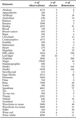
Table 1: Datasets used in the experimental studies
Datasets observations# of classes# of dimension# of
Abalone 4174 3 8 Appendicitis 106 2 7 Artificial 700 2 10 Australian 690 2 14 Balance 625 3 4 Banana 5300 2 2 Biodeg 1055 2 41 Blood 748 2 4 Breast-cancer 683 2 9 Bupa 345 2 6 Cleveland 297 5 13 Contraceptive 1473 3 9 Fertility 100 2 9 Haberman 306 2 3 Heart 270 2 13 Hepatitis 80 2 19 Hill-valley 2424 2 100 Led7digit 500 10 7 Madelon 2000 2 500 Magic 19020 2 10 Mammographic 830 2 5 Musk1 476 2 166 Musk2 6598 2 166 Newthyroid 215 3 5 Page-blocks 5472 5 10 Phoneme 5404 2 5 Pima 768 2 8 Ring 7400 2 20 Sonar 208 2 60 Spambase 4601 2 57 Tae 151 3 5 Tic-tac-toe 958 2 9 Titanic 2201 2 3 Vehicle 846 4 18 Vertebral 310 3 6 Waveform-w-noise 5000 3 40 Waveform-wo-noise 5000 3 21 Wdbc 569 2 30 Wine-red 1599 6 11 Wine-white 4898 7 11
row of the matrix corresponds to an observation, and it is obtained by concatenating all the predictions ofKbase classifiers.
There are two types of meta-classifiers introduced for the hetero-geneous ensemble systems: fixed combining methods and trainable combining methods. Fixed combining methods predict the label based on only the meta-data of the test sample. Kitller et al. [10] introduced six fixed combining rules (Sum, Product, Majority Vote, Min, Max, and Median) for an ensemble and pointed out that the Sum rule is the most reliable combining method for the prediction. Trainable combining methods, on the other hand, exploit the label information in the meta-data of the training set when constructing the meta-classifier. By doing this, trainable combining methods usually perform better than fixed combining methods.
In trainable combining methods, we can divide the combining methods into two categories, namely weight-based combining meth-ods and representation-based combining methmeth-ods. In the first cat-egory, the meta-classifier is formed based on the M weighted lin-ear combinations of posterior probabilities for the M classes. The weights can be computed using, for example, the Multi-Response Linear Regression (MLR) method [25], or the MLR plus hinge loss function [22]. On the other hand, the representation-based combin-ing methods generate a representation of the meta-data for each class label. The class label is assigned to a test sample based on the similarity between the set of representations and the meta-data of the test sample. Some examples of methods in this category are Decision Template [12], Bayesian-based combining method [19],
Granular-based prototype (interval-based representation) [18], and Fuzzy IF-THEN Rule-combining method [17].
2.2
Selection Methods in Ensemble System
In this section, we briefly introduce several selection methods ap-plied to ensemble system in which not only the base classifiers but also the features are selected to optimize the ensemble’s perfor-mance. We start with the ensemble selection (ES) methods (known by two different names: selective ensemble and ensemble prun-ing which are methods that search for a subset of classifiers that performs better than the whole ensemble. In ES, a single classifier or an ensemble of classifiers can be obtained using a static or a dynamic approach. The static approach selects a subset of base classifiers during the training phase and uses the same subset of base classifiers to predict all unseen samples. Nguyen et al. [15] proposed a novel encoding method that encodes both the base clas-sifiers and six fixed combining rules in a binary vector and used a Genetic Algorithm to search for the optimal EoC and the optimal fixed combining rule. Shunmugapriya and Kanmani [23] used the Artificial Bee Colony (ABC) algorithm to find the optimal set of base classifiers and the meta-classifier. Chen et al. [5] used the Ant Colony Optimization (ACO) algorithm to find the optimal set of base classifiers in the ensemble system with the Decision Tree as the meta-classifier. Zhang et al. [27] formulated the ES problem as a quadratic integer programming problem and used semi-definite programming to obtain an approximate solution.
Meanwhile, the dynamic approach selects a classifier by dynamic classifier selection (DCS) or an EoC by dynamic ensemble selection (DES) with the most competences in a defined region associated with each test sample. Some examples of DCS and DES methods are MLA [24], KNOP [4], KNORA Union and KNORA Eliminate [11], and Random Projection-based DES [7]. Comparison experiments in [3] indicated that simple dynamic selection methods like KNORA Union can sometimes perform better than the complex ones. A detailed review of methods for DCS and DES can be found in [3, 6]. Finally, we introduce some feature selection methods that were developed for ensemble systems. Kuncheva et al. [12] used a Venn diagram to encode the input features used by the learning algo-rithms and then search for the optimal set of input features and learning algorithms using GA. Nguyen et al. [14] developed a GA-based method to simultaneously learn the optimal EoC as well as the associated input features for the learning algorithm. The method introduced in [16] uses GA to find the optimal set of meta-data’s columns from the matrixLfor the Decision Tree meta-classifier.
3
PROPOSED METHOD
In this study, we introduce a method based on ACO to simultane-ously select a subset of meta-data’s columns fromLas well as the meta-classifier for a heterogeneous ensemble system. The columns of the meta-data are selected as paths by the ants. Each ant is also as-signed a certain meta-classifier. The subset of meta-data’s columns and the associated meta-classifier form a configuration of an ant. In each iteration, an ant tries to select a path in its route to obtain a better configuration. At the end of ACO, we select the best con-figuration based on an evaluation criterion. This optimal solution will be used to classify the test samples.
Local information ! "# "$ … "& … "'(
"#& )$& … "*& … "+,
& -$ - C ros s V ali da tio n ".&* Meta-data " Q Me ta -cl as si fi er s
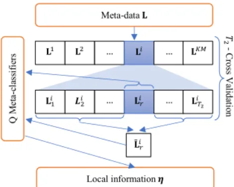
Figure 1: Module to compute the local information
Some notations that will be used in our algorithm are given below:
• Li: the meta-data associated with the columniofL
• Lij: thejthpart ofLi
• L{u}: the meta-data associated with the set of columnsu=
{u1,u2, ...,uk}ofL
• L{ju}: thejthpart ofL{u}
•na: the number of artificial ants in the colony
•τi: the pheromone associated with theithcolumn ofL
•ηi,q: the local information used to estimate the contribution of theithcolumn ofLto theqthmeta-classifier
•Sj: the configuration constructed by thejthant.
•αSj: the classification accuracy of configurationSj
• ρ: the evaporation rate,ρ∈[0,1]
•maxT: the maximum iteration number
In this framework,Klearning algorithms,Qmeta-classifiers, and the training setDare given. We start with the meta-data generated from the training setDusing theT1-fold cross validation procedure.
Specifically, the training setDis partitioned to obtainT1disjoint
partsD=D1∪...∪DT1,Dl∩Dr =∅(l,r), and|D1| ≈...≈
|DT
1|. The meta-data of observations inDr is then formed by the classifiers generated by learning theKalgorithms onDHr =D−Dr.
The meta-data of all training observations belonging toDis finally obtained by concatenating all meta-data from eachDr into the form of matrixLgiven by (1).
We then calculate the local information of each column ofLand the meta-classifier. This is the guide for an ant to search in the local area to find the new path. To calculateηi,q, aT2-fold cross
validation procedure is applied to the columnLiof the meta-data. We first obtainT2disjoint partsLi = Li1∪...∪LTi
2,L i l ∩Lir = ∅(l,r), and|Li1| ≈...≈ |LiT 2|. Predictions of observations inL i r
is then formed by theqthmeta-classifier trained onHL
i
r =Li−Lir. Predictions of all training data belonging toLiis finally obtained by gathering all predictions from eachLir. The average accuracy of the
qthmeta-classifier over all observations inLiis used as the local informationηi,q(see Figs 1). We also initialize the pheromoneτi
of each columnLi with a small positive number for the probability selection process.
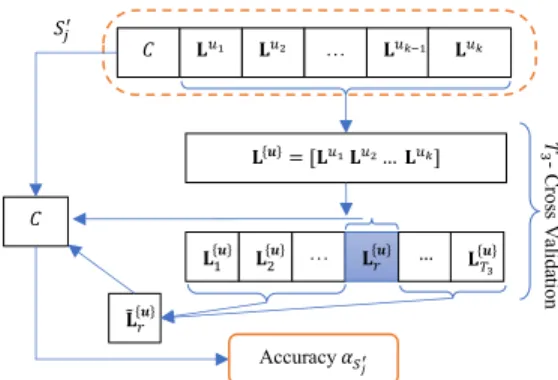
! " - C ros s V ali da tion # $%& $%' … $%()& $%( ${+}= [$%& $%'… $%(] $2{+} ${+}3 … ${+}4 … $56 {+} # $7{+}4 Accuracy 89:; <=>
Figure 2: Module to compute the evaluation criterion of a configuration
In the first step of each iteration in the ACO algorithm, each ant is randomly given a meta-classifier (uniform distribution). In the following steps, when thejthant begins its configuration search, it tries to select a columnLifromLwhich does not exist in its current configurationSj using roulette wheel selection. The probabilitypi
of the columnLito be selected by thejthant with the associated
qthmeta-classifier is computed based on the pheromone of each column and the local information as:
pi= τi×ηi,q Pm t=1,Lt<Sjτt×ηt,q ifL i <Sj 0 otherwise (2) We define the evaluation criterion for configurationSjasαSj. Dur-ing the ACO main process, suppose that the current configura-tion of an ant isSj = {C,Lu1,Lu2, ...,Luk−1}and a columnLi is selected, a new configurationS′j = {C,Lu1,Lu2, ...,Luk−1,Luk = Li}={C,L{u}}of this ant is generated. ThenS′
jis tested by usingT3
-fold cross validation on the corresponding subset of the meta-data in its configuration to calculateαS′
j. Specifically,L
{u}is partitioned
intoT3disjoint partsL{u}=L1{u}∪...∪LT{u}
3 ,L {u} l ∩L {u} r =∅(l,r), and|L1{u}| ≈ ... ≈ |LT{u} 3 |. Predictions of observations inL {u} r is then formed by the meta-classifierCtrained onHL
{u}
r =L{u}−Lr{u}. Based on the predictions of observations inLr{u}, we compute the loss functionL0−1{Lr{u},Sj′}by (3). The evaluation criterionαS′
jof configurationS′jis computed as the average classification accuracy for allLr{u}r=1, ...,T3(Fig. 2)
L0−1{Lr{u},Sj′}= 1 |Lr{u}| X x∈L{ru} I[yx,predict(Sj′,x)] (3) L0−1(S′j)= 1 T3 T3 X r=1 L0−1{Lr{u},Sj′} (4) αS′ j =1− L0−1(S ′ j) (5)
where predict(Sj′,x)returns the predicted class label for observation xby using the configurationSj′andyx is the true label ofx. If the performance ofS′jis better thanSj, it will replaceSj and the ant continues to find another column using the same strategy to
generate a new configuration. IfSj′cannot improve the accuracy of
Sj, this ant keeps its current configuration and stops its search in the iteration. During the ants’ searching process, once a columnLi is chosen to be added to anySjto form a better configurationS′
j, the
pheromone ofLi will accumulate, thus enhancing the probability of this column being selected by other ants. The improvement of accuracy fromSjtoS′jis used to update the pheromone ofLi. The update rule for the improvement is given in (6).
τi(new)=τi(old)+CC×τi(old)×
αS′ j−αSj
αSj
(6) whereCCrefers to a constant number. The pheromones of all candidates will evaporate after each iteration. The evaporation rule is given in (7).
τi(new) ←τi(old)×(1−ρ) (7) Therefore, the pheromone of the strong candidates will accumulate and the pheromone of the poor ones will vanish by evaporation. The evaporation rateρandCCare introduced to adjust the emphasis of historical knowledge and the current knowledge. The greaterρ
is, the less historical information will be used. The greaterCCis, the more important current knowledge is considered.
When we finish looping through all iterations, the best config-urationSbest among allnaants will be chosen as the final con-figuration. To speed up the training process, we mark and save all the configurations which have already been explored by arti-ficial ants in the past. So that we do not need to recalculate the evaluation criterion for the visited configurations. Once we obtain the final configuration for our ensemble using cross-validation, all the base classifiers are trained on the entire training setDfor the predictions on the testing set later. The pseudo code of the training process of the proposed method is presented in Algorithm 1, 2 and 3 in the Supplement Material.
The testing process uses the base classifiers and the best config-urationSbest. For each unlabeled samplextest, we first obtain its meta-dataL(xtest)by using the base classifers. Based on the best configurationSbest, we get the corresponding subset of columns LI(xtest)and the meta-classifierCassociated with these columns. By applyingCtoLI(xtest), we get the prediction for the class label ofxtest. The pseudo code of the testing process is presented in Algorithm 4 in the Supplement Material.
4
EXPERIMENTAL STUDIES
4.1
Datasets and Experimental Settings
We conducted experiments on 40 datasets to evaluate the perfor-mance of the proposed method. The datasets are selected to be diverse in the number of class labels, the number of observations, and the number of dimensions. Information about the datasets used in the experiment is given in Table 1.
We compared the proposed method to some classifier selection and feature selection methods developed for the heterogeneous ensemble systems. The benchmark algorithms we selected includ-ing: ACO-S1 [5], GA Meta-data [16], KNORA Union and KNORA Eliminate [11]. In these benchmark algorithms, we used the same learning algorithms as in the proposed method. For ACO-S1, the Decision Tree works as the meta-classifier like in the original paper.
!"#$> !"#? Update pheromone '(= '(* Evaporation True + = 1, './01= ∅, !"3456= −∞ 9 = 1 '(= [;, ∅], !"#= −∞
Randomly select a meta-classifier ;
Try selecting feature =>
No feature can be selected? '(*= '(∪ => Calculate !"#$ (Fig 2) 9 = 9 + 1 9 ≤ BC? + ≤ DCE+? + = + + 1 Meta-data F
Local information G(Fig 1)
'./01= (!"#> !"3456) ? '(∶ './01 LM LN … LP … LQR LSP + T - Cr os s V ali da tio n
U Learning Algs Training set L Q Meta-classifiers
Output './01 True False False True False True False Base classifiers
Figure 3: Training process of the proposed method The other parameters were set similar to the original paper. For
GA, the number of generations and the number of individuals in each generation was set to 100 and 50, respectively. For KNORA Union and KNORA Eliminate, the number of nearest neighbors was set to 7 as it is the best value for the DES method [6]. For the ACO algorithm to search for the optimal solution in the proposed method, we setmaxT =100,na =50,ρ =0.1, andCC =1. For the cross validation procedures to generate the meta-data of the training set, to calculate the local information, and the evaluation criteria, we setT1=10,T2=T3=2.
In this study, we performed 10-fold cross validation and ran the test 3 times to obtain 30 test results of each method on each
dataset. Based on the experimental results, we used the Wilcoxon signed rank test [8] to compare the classification results of the proposed method and each benchmark algorithm on each dataset. The null hypothesis is "there is no statistically significant difference in the results produced by the two methods". The null hypothesis is rejected if the p-value of the test is smaller than a given significance level, which we set to 0.05.
4.2
Results and Discussions
We first used 3 learning algorithms, namely Linear Discriminant Analysis (denoted by LDA), Naïve Bayes, andkNearest Neighbor
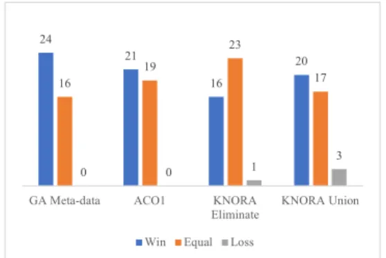
24 21 16 20 16 19 23 17 0 0 1 3
GA Meta-data ACO1 KNORA
Eliminate KNORA Union
Win Equal Loss
Figure 4: The Wilcoxon statistical test results (using 3 learning algorithms) 30 26 30 22 10 14 10 17 0 0 0 1
GA Meta-data ACO1 KNORA
Eliminate KNORA Union Win Equal Loss
Figure 5: The Wilcoxon statistical test results (using 7 learning algorithms)
Table 2: The classification error of the proposed method and the benchmark algorithms (using 3 learning algorithms)
GA Meta-data ACO-S1 KNORA Eliminate KNORA Union Proposed Method
Mean Variance Mean Variance Mean Variance Mean Variance Mean Variance
Abalone 0.4736• 5.43E-04 0.4720• 7.98E-04 0.4678 4.90E-04 0.4707• 3.88E-04 0.4576 3.99E-04
Appendicitis 0.1600 1.04E-02 0.1827 1.51E-02 0.1291 1.14E-02 0.1133□ 8.38E-03 0.1415 9.27E-03
Artificial 0.2295 2.39E-03 0.2257 2.41E-03 0.2257 1.98E-03 0.2171 1.23E-03 0.2310 1.57E-03
Australian 0.1807• 1.30E-03 0.1816• 2.38E-03 0.1589• 1.52E-03 0.1357 1.06E-03 0.1333 1.01E-03
Balance 0.0852 1.10E-03 0.0960 8.14E-04 0.1184• 3.27E-04 0.1093• 3.92E-04 0.0912 8.87E-04
Banana 0.1116 1.23E-04 0.1129 2.32E-04 0.1157 1.62E-04 0.1079□ 1.51E-04 0.1131 1.12E-04
Biodeg 0.1836• 1.22E-03 0.1800• 1.21E-03 0.1479 6.67E-04 0.1479 7.16E-04 0.1393 9.21E-04
Blood 0.2344 6.75E-04 0.2820• 2.86E-03 0.2286 1.32E-03 0.2205 8.87E-04 0.2348 2.32E-03
Breast-cancer 0.0420• 8.14E-04 0.0405 6.97E-04 0.0410 7.67E-04 0.0444• 6.95E-04 0.0356 6.97E-04
Bupa 0.3804• 8.55E-03 0.3548 5.43E-03 0.3469• 2.47E-03 0.3373 3.13E-03 0.3197 4.80E-03
Cleveland 0.4433• 4.06E-03 0.4643• 6.10E-03 0.4162 3.06E-03 0.4038 3.37E-03 0.4027 6.28E-03
Contraceptive 0.5237• 1.30E-03 0.5028• 1.95E-03 0.4639 2.01E-03 0.4574 1.16E-03 0.4652 1.44E-03
Fertility 0.1900• 1.29E-02 0.1467 3.16E-03 0.1367 2.99E-03 0.1333 2.89E-03 0.1300 3.43E-03
Haberman 0.2964 2.26E-03 0.2984 1.72E-03 0.2778 1.82E-03 0.2767 1.80E-03 0.2823 2.26E-03
Heart 0.2395• 6.93E-03 0.2185• 8.26E-03 0.1938 5.18E-03 0.1753 3.65E-03 0.1716 3.52E-03
Hepatitis 0.1750 1.42E-02 0.2083 9.72E-03 0.1458 7.38E-03 0.1458 9.46E-03 0.1750 8.96E-03
Hill-valley 0.2745 2.47E-03 0.2785 3.54E-03 0.3228• 1.29E-03 0.4086• 1.60E-03 0.2629 3.48E-03
Led7digit 0.2973• 4.50E-03 0.3013• 6.05E-03 0.2680□ 4.82E-03 0.2653□ 3.86E-03 0.2860 4.22E-03
Madelon 0.2870 6.94E-04 0.2870 6.94E-04 0.3287• 8.82E-04 0.3787• 1.14E-03 0.2873 8.98E-04
Magic 0.1920• 1.37E-04 0.1902• 4.75E-05 0.1934• 5.56E-05 0.1933• 4.80E-05 0.1887 4.13E-04
Mammographic 0.2032• 1.97E-03 0.2169• 1.76E-03 0.1855 1.90E-03 0.1851 1.58E-03 0.1827 1.17E-03
Musk1 0.1344• 1.61E-03 0.1245• 1.77E-03 0.1708• 2.28E-03 0.1695• 3.87E-03 0.1001 1.30E-03
Musk2 0.0350 3.46E-05 0.0355 3.45E-05 0.0356 4.37E-05 0.0498• 7.44E-05 0.0368 5.94E-05
Newthyroid 0.0371 1.22E-03 0.0418• 1.36E-03 0.0947• 3.74E-03 0.0900• 2.60E-03 0.0576 2.64E-03
Page-blocks 0.0420 4.35E-05 0.0462 7.31E-05 0.0424 5.44E-05 0.0503• 5.14E-05 0.0437 5.54E-05
Phoneme 0.1149 2.11E-04 0.1149 2.11E-04 0.1337• 1.77E-04 0.1796• 3.30E-04 0.1208 1.25E-03
Pima 0.3056• 2.34E-03 0.3078• 2.35E-03 0.2366 2.31E-03 0.2427 2.84E-03 0.2318 2.47E-03
Ring 0.1232• 1.83E-04 0.1211• 1.30E-04 0.2590• 1.37E-04 0.2148• 8.96E-05 0.1162 1.55E-04
Sonar 0.2583• 8.89E-03 0.2368 5.91E-03 0.2375 8.11E-03 0.2437 5.70E-03 0.2162 8.55E-03
Spambase 0.1185• 1.95E-04 0.1224• 2.96E-04 0.1072• 1.23E-04 0.0977 9.32E-05 0.0960 2.15E-04
Tae 0.5453• 1.35E-02 0.5129 1.30E-02 0.4863 1.32E-02 0.4925 1.57E-02 0.4794 1.67E-02
Tic-tac-toe 0.1166 7.12E-04 0.1166 7.12E-04 0.1754• 7.50E-04 0.2220• 9.42E-04 0.1183 6.73E-04
Titanic 0.2160 3.81E-04 0.2178 4.08E-04 0.2282 9.77E-04 0.2260 6.16E-04 0.2425 5.19E-03
Vehicle 0.2627• 1.90E-03 0.2597• 1.44E-03 0.2651• 2.13E-03 0.2569• 1.11E-03 0.2203 1.09E-03
Vertebral 0.1893• 3.38E-03 0.1527 3.46E-03 0.1753 4.21E-03 0.1968• 4.39E-03 0.1581 2.87E-03
Waveform-w-noise 0.1787• 2.04E-04 0.1770• 2.22E-04 0.1647• 2.81E-04 0.1692• 1.79E-04 0.1479 1.71E-04
Waveform-wo-noise 0.1738• 4.45E-04 0.1705• 2.75E-04 0.1569• 2.79E-04 0.1653• 2.93E-04 0.1605 1.48E-02
Wdbc 0.0352 6.19E-04 0.0457• 8.53E-04 0.0475• 9.50E-04 0.0399• 3.09E-04 0.0293 3.97E-04
Wine-red 0.4653• 2.14E-03 0.4690• 1.05E-03 0.4180 8.78E-04 0.4234• 1.19E-03 0.4084 8.95E-04
Wine-white 0.4798• 4.58E-04 0.4947• 6.21E-04 0.4502 4.67E-04 0.4682• 3.06E-04 0.4524 5.60E-04
Average ranking 3.43 3.5 3.09 2.95 2.04
•and□mean the proposed method is better or worse than the benchmark algorithm, respectively.
(kwas set to 5, denoted bykNN5) [17, 19] to construct the
het-erogeneous ensemble system. The set of meta-classifiers was set similarly to the set of learning algorithms. The experimental results of the proposed method and 4 benchmark algorithms were shown in Table 2.
Clearly, the proposed method is better than the benchmark algo-rithms on the datasets. Compared to ACO-S1, the proposed method
wins on 21 datasets. Our method significantly outperforms GA Meta-data, winning on 24 datasets and does not lose on any datasets. The proposed method is also better than the two DES method, as our method win KNORA Union and KNORA Eliminate on 16 and 20 datasets, respectively. We also computed the average ranking of all methods based on their experimental results. It once again shows the outstanding performance of the proposed method as our
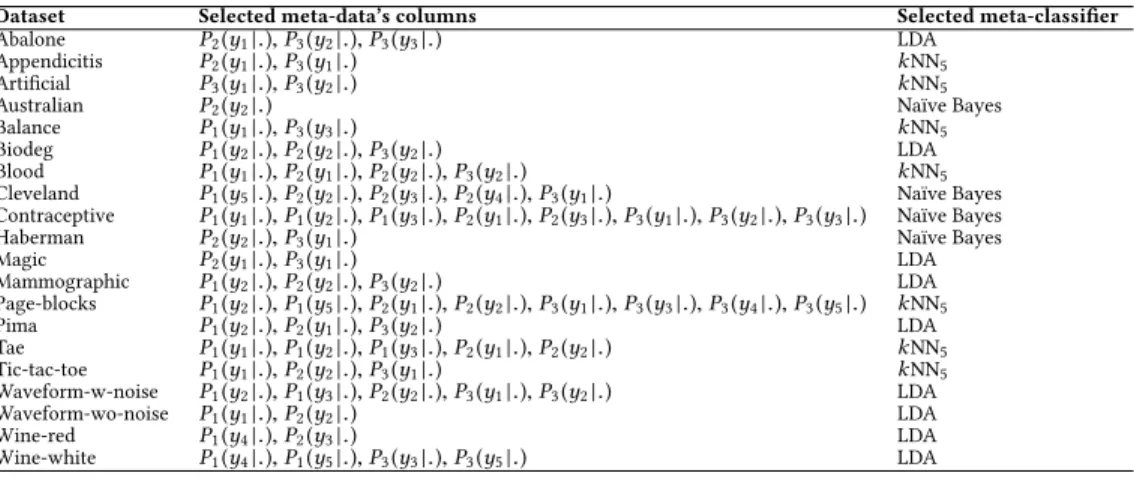
Table 3: The selected meta-data’s columns and meta-classifier for 20 experimental datasets (using 3 classifiers)
Dataset Selected meta-data’s columns Selected meta-classifier
Abalone P2(y1|.),P3(y2|.),P3(y3|.) LDA
Appendicitis P2(y1|.),P3(y1|.) kNN5
Artificial P3(y1|.),P3(y2|.) kNN5
Australian P2(y2|.) Naïve Bayes
Balance P1(y1|.),P3(y3|.) kNN5
Biodeg P1(y2|.),P2(y2|.),P3(y2|.) LDA
Blood P1(y1|.),P2(y1|.),P2(y2|.),P3(y2|.) kNN5
Cleveland P1(y5|.),P2(y2|.),P2(y3|.),P2(y4|.),P3(y1|.) Naïve Bayes
Contraceptive P1(y1|.),P1(y2|.),P1(y3|.),P2(y1|.),P2(y3|.),P3(y1|.),P3(y2|.),P3(y3|.) Naïve Bayes
Haberman P2(y2|.),P3(y1|.) Naïve Bayes
Magic P2(y1|.),P3(y1|.) LDA Mammographic P1(y2|.),P2(y2|.),P3(y2|.) LDA Page-blocks P1(y2|.),P1(y5|.),P2(y1|.),P2(y2|.),P3(y1|.),P3(y3|.),P3(y4|.),P3(y5|.) kNN5 Pima P1(y2|.),P2(y1|.),P3(y2|.) LDA Tae P1(y1|.),P1(y2|.),P1(y3|.),P2(y1|.),P2(y2|.) kNN5 Tic-tac-toe P1(y1|.),P2(y2|.),P3(y1|.) kNN5 Waveform-w-noise P1(y2|.),P1(y3|.),P2(y2|.),P3(y1|.),P3(y2|.) LDA Waveform-wo-noise P1(y1|.),P2(y2|.) LDA Wine-red P1(y4|.),P2(y3|.) LDA Wine-white P1(y4|.),P1(y5|.),P3(y3|.),P3(y5|.) LDA
Table 4: The classification error of the proposed method and the benchmark algorithms (using 7 learning algorithms)
GA Meta-data ACO-S1 KNORA Eliminate KNORA Union Proposed Method
Mean Variance Mean Variance Mean Variance Mean Variance Mean Variance
Abalone 0.4986• 6.84E-04 0.4888• 9.25E-04 0.4812• 6.90E-04 0.4652• 4.42E-04 0.4534 4.10E-04
Appendicitis 0.1767• 9.44E-03 0.1630 1.18E-02 0.1424 8.98E-03 0.1261 9.77E-03 0.1324 1.01E-02
Artificial 0.2667• 3.80E-03 0.2229 2.14E-03 0.2538 1.89E-03 0.2210 1.70E-03 0.2476 4.18E-03
Australian 0.1845• 1.97E-03 0.1908• 2.62E-03 0.1826• 2.30E-03 0.1541 1.63E-03 0.1401 1.32E-03
Balance 0.0491 1.08E-03 0.0581 1.13E-03 0.1157• 1.12E-03 0.1029• 4.99E-04 0.0597 1.00E-03
Banana 0.1331• 3.65E-04 0.1279• 3.51E-04 0.1184• 2.10E-04 0.1029• 8.77E-05 0.0991 9.84E-05
Biodeg 0.1773• 1.19E-03 0.1839• 1.16E-03 0.1823• 1.86E-03 0.1422• 8.31E-04 0.1273 6.66E-04
Blood 0.2861• 3.18E-03 0.2643• 1.46E-03 0.2664• 2.52E-03 0.2254 1.35E-03 0.2241 1.53E-03
Breast-cancer 0.0483• 7.88E-04 0.0449• 7.01E-04 0.0454• 7.62E-04 0.0434 8.81E-04 0.0371 5.23E-04
Bupa 0.3585• 5.38E-03 0.3606• 8.10E-03 0.3446 6.94E-03 0.2955 3.57E-03 0.3112 6.66E-03
Cleveland 0.4615• 5.21E-03 0.4631• 6.00E-03 0.4847• 7.82E-03 0.4251 3.20E-03 0.4051 5.19E-03
Contraceptive 0.5230• 1.59E-03 0.5130• 2.00E-03 0.4795• 1.69E-03 0.4415 1.64E-03 0.4410 1.34E-03
Fertility 0.1967• 1.50E-02 0.1833 1.54E-02 0.1733 9.29E-03 0.1267 3.96E-03 0.1433 5.79E-03
Haberman 0.3474• 4.33E-03 0.3312• 4.55E-03 0.2962 2.09E-03 0.2846 1.90E-03 0.2865 2.33E-03
Heart 0.2370• 6.46E-03 0.2185• 3.78E-03 0.2543• 7.02E-03 0.1889 4.60E-03 0.1778 2.78E-03
Hepatitis 0.2125 2.62E-02 0.1917 8.06E-03 0.1625 1.58E-02 0.1417 1.33E-02 0.1875 1.43E-02
Hill-valley 0.0868 1.39E-02 0.0823 1.58E-02 0.6179• 1.40E-01 0.3715• 4.97E-03 0.0679 5.59E-03
Led7digit 0.3293• 4.69E-03 0.3013• 5.20E-03 0.2947 5.09E-03 0.2673□ 4.65E-03 0.2820 4.70E-03
Madelon 0.2370• 1.82E-03 0.2222 9.83E-04 0.3028• 6.19E-04 0.3060• 1.67E-03 0.2172 7.03E-04
Magic 0.2042• 1.89E-04 0.1735• 4.94E-05 0.1805• 5.87E-05 0.1726• 5.77E-05 0.1487 3.94E-05
Mammographic 0.2237• 2.55E-03 0.2092• 2.35E-03 0.2149• 1.96E-03 0.1851 1.20E-03 0.1799 1.78E-03
Musk1 0.0889• 1.73E-03 0.1002• 2.69E-03 0.1274• 3.13E-03 0.1534• 3.23E-03 0.0588 1.31E-03
Musk2 0.0062 8.10E-06 0.0076 5.82E-05 0.0168• 2.38E-05 0.0342• 3.81E-05 0.0056 1.18E-05
Newthyroid 0.0354 1.51E-03 0.0374 1.70E-03 0.0760• 4.46E-03 0.0761• 2.72E-03 0.0374 1.09E-03
Page-blocks 0.0355 5.84E-05 0.0370• 4.09E-05 0.0416• 3.68E-05 0.0478• 4.81E-05 0.0337 5.73E-05
Phoneme 0.1271• 4.04E-04 0.1172• 2.39E-04 0.1297• 1.85E-04 0.1462• 3.54E-04 0.1075 1.67E-04
Pima 0.3047• 3.03E-03 0.3077• 2.45E-03 0.2891• 1.88E-03 0.2435 2.57E-03 0.2370 2.01E-03
Ring 0.0301• 3.19E-05 0.0305• 3.70E-05 0.0985• 1.35E-04 0.1019• 5.30E-04 0.0211 4.46E-05
Sonar 0.2114• 7.56E-03 0.2391• 6.54E-03 0.1949 1.30E-02 0.2160• 7.41E-03 0.1634 6.77E-03
Spambase 0.0805• 1.43E-04 0.0826• 1.41E-04 0.1222• 3.22E-03 0.0845• 3.01E-04 0.0823 1.55E-02
Tae 0.4989 1.42E-02 0.0826 1.41E-04 0.4614 1.10E-02 0.4881 1.93E-02 0.4682 1.52E-02
Tic-tac-toe 0.0327 4.42E-04 0.0394 4.81E-04 0.0553• 4.31E-04 0.1204• 1.00E-03 0.0317 2.87E-04
Titanic 0.2267 1.79E-03 0.2161 3.26E-04 0.2359• 2.31E-03 0.2255• 5.97E-04 0.2170 3.68E-04
Vehicle 0.2514• 2.27E-03 0.2692• 1.68E-03 0.2972• 1.50E-03 0.2872• 1.23E-03 0.2242 9.85E-04
Vertebral 0.2022• 3.88E-03 0.1828 4.81E-03 0.1785 4.84E-03 0.1742 3.44E-03 0.1570 2.69E-03
Waveform-w-noise 0.1755• 2.45E-04 0.1725• 1.94E-04 0.1979• 7.42E-04 0.1641• 1.51E-04 0.1392 2.12E-04
Waveform-wo-noise 0.1773• 3.82E-04 0.1739• 2.44E-04 0.1783• 5.67E-04 0.1597• 3.92E-04 0.1346 3.12E-04
Wdbc 0.0392 5.48E-04 0.0369 6.24E-04 0.0545• 8.89E-04 0.0393 4.87E-04 0.0322 4.15E-04
Wine-red 0.4534• 1.86E-03 0.4332• 2.49E-03 0.4263• 1.84E-03 0.3900• 8.16E-04 0.3700 1.07E-03
Wine-white 0.4879• 7.54E-04 0.4578• 7.22E-04 0.4610• 8.94E-04 0.4226• 5.52E-04 0.4027 5.59E-04
Average ranking 3.73 3.26 3.8 2.8 1.41
•and□mean the proposed method is better or worse than the benchmark algorithm, respectively.
method rank first (with rank value of 2.04), followed by KNORA Union and KNORA Eliminate (with rank value of 2.95 and 3.09, respectively).
Compared to the benchmark algorithms, our approach has sev-eral advantages that explain the superior performance. First, GA Meta-data uses GA to select the meta-data’s columns while fixes
the meta-classifier, making it less flexible than our method. ACO-S1, meanwhile, selects the base classifiers and also fixes the meta-classifier.
Table 3 shows some examples of the selected meta-data’s columns and meta-classifier of the proposed method. As mentioned before, instead of using classifier selection that removes all predictions of
a classifier if it is not selected, we selected a subset of its prediction and a suitable meta-classifier. This makes our model more general and better than ACO-S1. Finally, the two DES methods perform poorer than our method because their performance depends on the choice of techniques that define the region associated with each test sample [6]. The average training time of proposed method com-puted on 30 test rounds on Abalone dataset is 3 seconds compared to 0.5 and 0.3 seconds of ACO-S1 and GA Meta-data, respectively. Although proposed method generally has longer running time than ACO-S1 and GA Meta-data, the differences are within practical limit.
4.3
Different number of learning algorithms
To evaluate the influence of using different number of learning algorithms on the ensemble performance, we added four learning algorithms to the previous set of learning algorithms introduced in Section 4.2. The newly added learning algorithms are Decision Tree, LibLinear [9], Nearest Mean Classifier, and Discriminative Restricted Boltzmann Machines [13]. The set of meta-classifiers were selected to be the same as the set of learning algorithms. The experimental results of the proposed method and the benchmark algorithms with the new ensemble system are shown in Table 3. The statistical test results in Fig. 5 once again show the superior performance of the proposed method compared to the benchmark algorithms: we win KNORA Eliminate and GA Meta-data on 30 datasets, wins ACO-S1 on 26 datasets and win KNORA Union on 22 datasets. The proposed method only loses KNORA Union on 1 dataset.
5
CONCLUSIONS
In summary, we have introduced a method to simultaneously select a subset of meta-data and a meta-classifier for the heterogeneous ensemble system to obtain higher classification accuracy than using the entire meta-data with one fixed meta-classifier. Our method first uses the cross validation procedure on the training dataset with the given learning algorithms to obtain the base classifiers and the meta-data. Having obtained the meta-data and the given set of meta-classifiers, we applied ACO to search for the optimal subset of meta-data and the associated meta-classifier. An ant will search around the local area based on the local information. In this study, we defined the local information as the classification accuracy associated with each meta-data’s column and meta-classifier. Each ant’s configuration including the candidate solution is evaluated by using another cross validation procedure on the selected meta-data. After ACO, we obtain the best configuration consisting of the subset of meta-data’s columns and the associated meta-classifier for the ensemble. The classification process works in a straightforward manner by employing the best configuration on the test samples. Experiments conducted on 40 UCI datasets show that the proposed method is better than the benchmark algorithms we compared concerning the classification accuracy.
REFERENCES
[1] Iñigo Barandiaran. 1998. The random subspace method for constructing decision forests.IEEE transactions on pattern analysis and machine intelligence20, 8 (1998).
[2] Leo Breiman. 1996. Bagging predictors.Machine learning24, 2 (1996), 123–140.
[3] Alceu S Britto Jr, Robert Sabourin, and Luiz ES Oliveira. 2014. Dynamic selection
of classifiers - a comprehensive review.Pattern Recognition47, 11 (2014), 3665–
3680.
[4] Paulo R Cavalin, Robert Sabourin, and Ching Y Suen. 2013. Dynamic selection
approaches for multiple classifier systems.Neural Computing and Applications
22, 3-4 (2013), 673–688.
[5] Yijun Chen, Man-Leung Wong, and Haibing Li. 2014. Applying Ant Colony
Optimization to configuring stacking ensembles for data mining.Expert systems
with applications41, 6 (2014), 2688–2702.
[6] Rafael MO Cruz, Robert Sabourin, and George DC Cavalcanti. 2018. Dynamic
classifier selection: Recent advances and perspectives. Information Fusion41
(2018), 195–216.
[7] Manh Truong Dang, Anh Vu Luong, Tuyet-Trinh Vu, Quoc Viet Hung Nguyen, Tien Thanh Nguyen, and Bela Stantic. 2018. An Ensemble System with Random
Projection and Dynamic Ensemble Selection. InAsian Conference on Intelligent
Information and Database Systems. Springer, 576–586.
[8] Janez Demšar. 2006. Statistical comparisons of classifiers over multiple data sets. Journal of Machine learning research7, Jan (2006), 1–30.
[9] Rong-En Fan, Kai-Wei Chang, Cho-Jui Hsieh, Xiang-Rui Wang, and Chih-Jen Lin.
2008. LIBLINEAR: A library for large linear classification.Journal of machine
learning research9, Aug (2008), 1871–1874.
[10] Josef Kittler, Mohamad Hatef, Robert PW Duin, and Jiri Matas. 1998. On
combin-ing classifiers.IEEE transactions on pattern analysis and machine intelligence20,
3 (1998), 226–239.
[11] Albert HR Ko, Robert Sabourin, and Alceu Souza Britto Jr. 2008. From dynamic classifier selection to dynamic ensemble selection.Pattern Recognition41, 5 (2008), 1718–1731.
[12] Ludmila I Kuncheva, James C Bezdek, and Robert PW Duin. 2001. Decision
templates for multiple classifier fusion: an experimental comparison. Pattern
recognition34, 2 (2001), 299–314.
[13] Hugo Larochelle and Yoshua Bengio. 2008. Classification using discriminative
restricted Boltzmann machines. InProceedings of the 25th international conference
on Machine learning. ACM, 536–543.
[14] Tien Thanh Nguyen, Alan Wee-Chung Liew, Xuan Cuong Pham, and Mai Phuong Nguyen. 2014. A novel 2-stage combining classifier model with stacking and genetic algorithm based feature selection. InInternational Conference on Intelligent Computing. Springer, 33–43.
[15] Tien Thanh Nguyen, Alan Wee-Chung Liew, Xuan Cuong Pham, and Mai Phuong Nguyen. 2014. Optimization of ensemble classifier system based on multiple objectives genetic algorithm. (2014), 46–51 pages.
[16] Tien Thanh Nguyen, Alan Wee-Chung Liew, Minh Toan Tran, Xuan Cuong Pham, and Mai Phuong Nguyen. 2014. A novel genetic algorithm approach for simultaneous feature and classifier selection in multi classifier system. In Evolutionary Computation (CEC), 2014 IEEE Congress on. IEEE, 1698–1705. [17] Tien Thanh Nguyen, Mai Phuong Nguyen, Xuan Cuong Pham, and Alan
Wee-Chung Liew. 2018. Heterogeneous classifier ensemble with fuzzy rule-based meta
learner.Information Sciences422 (2018), 144–160.
[18] Tien Thanh Nguyen, Mai Phuong Nguyen, Xuan Cuong Pham, Alan Wee-Chung Liew, and Witold Pedrycz. 2018. Combining heterogeneous classifiers via granular
prototypes.Applied Soft Computing73 (2018), 795–815.
[19] Tien Thanh Nguyen, Thi Thu Thuy Nguyen, Xuan Cuong Pham, and Alan Wee-Chung Liew. 2016. A novel combining classifier method based on Variational
Inference.Pattern Recognition49 (2016), 198–212.
[20] Tien Thanh Nguyen, Xuan Cuong Pham, Alan Wee-Chung Liew, and Witold Pedrycz. 2018. Aggregation of classifiers: a justifiable information granularity
approach.IEEE Transactions on Cybernetics(2018).
[21] Simon Parsons. 2005. Ant Colony Optimization by Marco Dorigo and Thomas
Stützle, MIT Press, 305 pp., 40.00, ISBN 0-262-04219-3.The Knowledge Engineering
Review20, 1 (2005), 92–93.
[22] Mehmet Umut ŞEn and Hakan Erdogan. 2013. Linear classifier combination and
selection using group sparse regularization and hinge loss.Pattern Recognition
Letters34, 3 (2013), 265–274.
[23] Palanisamy Shunmugapriya and S Kanmani. 2013. Optimization of stacking
ensemble configurations through artificial bee colony algorithm. Swarm and
Evolutionary Computation12 (2013), 24–32.
[24] Paul C Smits. 2002. Multiple classifier systems for supervised remote sensing
image classification based on dynamic classifier selection.IEEE Transactions on
Geoscience and Remote Sensing40, 4 (2002), 801–813.
[25] Kai Ming Ting and Ian H Witten. 1999. Issues in stacked generalization.Journal
of artificial intelligence research10 (1999), 271–289.
[26] Chun-Xia Zhang and Robert PW Duin. 2011. An experimental study of one-and
two-level classifier fusion for different sample sizes.Pattern Recognition Letters
32, 14 (2011), 1756–1767.
[27] Yi Zhang, Samuel Burer, and W Nick Street. 2006. Ensemble pruning via
semi-definite programming.Journal of Machine Learning Research7, Jul (2006), 1315–