Full Terms & Conditions of access and use can be found at
http://www.tandfonline.com/action/journalInformation?journalCode=tcfm20
Download by: [Cranfield University] Date: 01 April 2016, At: 05:31
Engineering Applications of Computational Fluid
Mechanics
ISSN: 1994-2060 (Print) 1997-003X (Online) Journal homepage: http://www.tandfonline.com/loi/tcfm20
Computational study of a complex
three-dimensional shock boundary-layer interaction
Joshua Katzenberg & David MacManus
To cite this article: Joshua Katzenberg & David MacManus (2015) Computational study of a complex three-dimensional shock boundary-layer interaction, Engineering Applications of Computational Fluid Mechanics, 9:1, 259-279, DOI: 10.1080/19942060.2015.1007564
To link to this article: http://dx.doi.org/10.1080/19942060.2015.1007564
© 2015 The Author(s). Published by Taylor & Francis.
Published online: 06 Mar 2015.
Submit your article to this journal
Article views: 401
View related articles
Vol. 9, No. 1, 259–279, http://dx.doi.org/10.1080/19942060.2015.1007564
Computational study of a complex three-dimensional shock boundary-layer interaction
Joshua Katzenberg and David MacManus∗Department of Power and Propulsion, School of Engineering, Cranfield University, Cranfield, MK42 0AL, Bedfordshire, UK (Received 22 July 2014; final version received 11 January 2015)
Shock boundary–layer interactions occur in many high-speed aerodynamic flows and they can have a notable impact on design considerations due to the aerodynamic and heat transfer effects. Consequently there is a notable interest in under-standing the ability of computational tools to calculate the complex flow fields that can arise in a range of engineering applications. Three-dimensional complex shock boundary layer interaction studies are expensive in both time and compu-tational resources. Although recent studies have begun to focus on the use of more complex compucompu-tational methods such as large eddy simulations, the aim of this research is to assess the ability of steady Reynolds averaged Navier Stokes turbu-lence models to simulate the interaction of a planar shock impinging on a cylindrical body under supersonic conditions and to determine if these models have a role to play in engineering design applications. The performance of both eddy viscosity and Reynolds stress models are evaluated relative to an established experimental test case. The impact of Reynolds number and impinging shock strength are also considered. Of the eddy viscosity models it was shown that the Spalart-Allmaras model is unsuitable for this complex interaction and that the k-ε and Reynolds stress methods both gave notably better agreement with the measured surface static pressures. Overall it was considered that the Reynolds stress method was the best model as it also provided better agreement with the measured surface flow topology. It was concluded that, although a steady Reynolds averaged Navier Stokes approach has known limitations for this type of complex interaction, within an engineering context it can also provide useful results when applied appropriately.
Keywords: shock boundary layer interaction; boundary layer separation; Reynolds stress model; oblique shock interaction; multibody; supersonic
1. Introduction
The topic of shock boundary layer interactions (SBLI) is a broad subject which has been the focus of extensive research over many years. It is a complex, multifaceted topic, which is not yet fully understood and still causes significant difficulties in the design of a wide range of high-speed vehicles and aerospace components (Allen, Heaslet, & Nitzberg, 1947; Borovoy et al., 2013; Brosh & Kus-soy,1983; Chaplin et al.,2011; Délery,1999; Donaldson,
1944; Holden, Wadhams, MacLean, & Mundy,2010). Ini-tial investigations of nominally two-dimensional SBLIs were previously undertaken for aerofoils under supersonic conditions. For an aerofoil under high transonic condi-tions, a normal shock wave can form and interact with the boundary layer, typically on the suction side (Babin-sky & Harvey, 2011). In this interaction, compression waves form near the wall as the boundary layer is unable to support the rise in static pressure across the shock. As the shock strength increases, along with the concomi-tant adverse pressure gradient, boundary layer separation can occur. Further instances of nominally two-dimensional SBLIs have been investigated extensively, most notably
*Corresponding author. Email:d.g.macmanus@cranfield.ac.uk
for compression ramps and oblique shocks impinging on flat plates where it has been noted that the interaction depends on the nominal pressure rise across the shock as well as the state and characteristics of the approaching boundary layer (Arnal & Délery, 2004; Délery, Marvin, & Reshotko,1986; Délery, & Coet, 1990; Délery,1996). For example, an increase in the shock strength, by chang-ing the ramp angle, can lead to separation of the boundary layer if the pressure rise across the shock is high enough. Separation results in an influence from the SBLI which extends further upstream than with an attached SBLI and an additional shock system of separation and reattachment shocks can arise. Similar effects arise with the impinge-ment of a two-dimensional oblique shock onto a flat plate where the induced increase in the boundary layer thickness generates an additional shock wave ahead of the primary reflected shock which in turn crosses the impinging shock wave (Arnal & Délery, 2004). If the shock is of signifi-cant strength, an increase in the thickness of the boundary layer occurs and a separation bubble can also arise. Thus, in nominally two-dimensional SBLIs, shock strength and angle, dependant on Mach number and geometry, along
© 2015 The Author(s). Published by Taylor & Francis.
This is an Open Access article distributed under the terms of the Creative Commons Attribution License (http://creativecommons.org/licenses/by/4.0/), which permits unrestricted use, distribution, and reproduction in any medium, provided the original work is properly cited.
with the Reynolds number, state and shape factor of the approaching boundary layer are key parameters as to the nature of the shock interaction.
Nominally three-dimensional SBLIs are typically more complex and occur in many high-speed aerodynamic flows (Brosh & Kussoy, 1983; Pamadi et al.,2005). Examples include planar shocks impinging onto axisymmetric bod-ies (Brosh & Kussoy, 1983) and conical shock waves impinging onto flat plates (Gai & Teh, 2000). For these configurations, along the central symmetry plane there are broad similarities with the nominally two-dimensional SBLIs such as the local boundary layer thickening which can lead to separation. Critical factors which affect the likelihood and magnitude of separation are shock strength and shock angle which are typically controlled by the dis-tance of the shock generator from the boundary layer, approaching Mach number and the characteristics of the approaching boundary layer. For these configurations the increase in surface static pressure from the SBLI typically arises several boundary layer thicknesses upstream rela-tive to the nominal ideal shock impingement point and locally strong cross-flows can occur due to the SBLI. Dis-tinct regions arise within the flow field which depend on the initial SBLI and the subsequent evolution of the bound-ary layer, shock waves, expansion systems, crossflow and indeed the main flow (Chaplin et al.,2011). Adverse pres-sure gradients at the initial interaction point can be affected by lateral, or azimuthal, flow migration away from the position of peak shock intensity which results in potent cross-flows (Brosh & Kussoy, 1983). In the case of a planar oblique shock impinging onto a cylindrical body (Brosh & Kussoy,1983), the coalescing of the diffracted shocks on the leeward side resulted in an additional sep-aration region and thereby deflected the flow in a similar manner to an obstacle in the boundary layer (Peake & Tobak,1982; Sedney & Kitchens,1975). Further detailed studies of three-dimensional SBLIs are reported by other researchers (Arnal & Délery, 2004; Babinsky & Harvey,
2011; Peake & Tobak,1982; Saric et al.,1996).
1.1. Computational studies of SBLIs
SBLIs comprise a very wide range of configurations and flow regimes and the aerodynamic characteristics of the interaction is highly dependent on the defining conditions. The interactions can encompass aspects such as transi-tion, separatransi-tion, highly skewed boundary layers, reflected shocks and expansion fans, vortical flows and strongly three-dimensional flow gradients (Babinsky & Harvey,
2011). Furthermore, it is considered that all SBLIs are fundamentally unsteady to some degree (Oliver, Lillard, Schwing, Blaisdell, & Lyrintzis,2007). Overall these fea-tures present a very challenging problem for computa-tional fluid dynamics (CFD). Nevertheless, a broad vari-ety of SBLI problems have been tackled using a range
of computational methods with varying degrees of suc-cess (Bhagwandin & DeSpirito, 2011; Dolling, 2001; Oliver et al.,2007). These methods have included vari-ous forms of Reynolds Averaged Navier Stokes (RANS) approaches (DeBonis et al., 2010; Thivet, 2002; Val-let,2007), unsteady RANS (URANS) (Barakos, Doerffer, Hirsch, Dussauge, & Babinsky,2010; Hirsch,2010a; Sand-ham,2010), Detached Eddy Simulations (DES) (Garnier,
2009; Shams & Comte, 2010), Large Eddy Simula-tions (LES) (DeBonis et al., 2010; Eagle, Driscoll, & Benek,2012; Hadjadj,2012) and Direct Numerical Sim-ulations (DNS) (Adams,2000; Tokura & Maekwa,2011). Clearly these methods provide different levels of modeling fidelity and sophistication along with concomitant resource demands.
Oliver et al. (2007) examined the ability of some steady RANS methods, Spalart-Allmaras (SA), Menter’s Shear Stress Transport (SST) and Olsey and Coakley’s Lag model, to calculate SBLIs occurring on flat plates and a compression ramp at Mach numbers ranging between 2.87 and 6.0. Simulations of relatively benign SBLIs pro-duce results that are in reasonable agreement with exper-imental results. However, as shock strength increases, the SBLI becomes more difficult to determine computationally and the difference in accuracy of various RANS models becomes more apparent. It was found that the calcula-tion of too large a separacalcula-tion bubble as well as a region of upstream influence which arises in two-dimensional calculations can be improved with a three-dimensional computational model as this includes relief effects as well as the impact of the wind tunnel walls which arises in many experimental configurations. For these cases, RANS models generally calculate the inviscid flow field as well as the overall effects such as separation and the region of upstream influence to a level deemed adequate for most engineering design work. However, Oliver et al. (2007) showed that the thermal environment and interactions proved more difficult to compute. In addition, the detailed flow visualization and skin-friction-related distributions were adversely affected even if surface pressures correlated closely with experimental data. It was noted that the low-frequency shock unsteadiness, a result of large streamwise turbulent fluctuations observed in the experiment, was not captured by RANS models due to the averaging of turbu-lent fluctuations, and thus, there was no physical source for such effects in RANS models. This problem was par-tially addressed by reducing the grid aspect ratio near the separation region and of the three models tested, the sim-ple formulation of the one-equation SA model providing the lowest fidelity, with the lag model producing results in-between the SA and SST models (Oliver et al.,2007).
Subsequent studies on the ability of steady RANS methods to calculate the SBLI flow field showed that the accuracy depends greatly on the turbulence model (DeBonis et al.,2010). It was reported that for weak SBLIs of planar shocks impinging on a flat plate, differences in the
calculated streamwise velocity distributions were within 0.5% of each RANS turbulence model considered for the Menter SST, k-ωvariants and Spalart-Allmaras mod-els. However, as the shock intensity increased, the error in all the solutions also increased, although the relative error between each turbulence model was relatively con-sistent. Grid construction, either structured or unstructured, showed no discernible difference on the calculated flow fields. The most notable difference between models was within the separation region of the SBLI although due to the range of metrics used in the assessment it was difficult to determine a clearly superior method. LES simulations were found to produce similar error levels as RANS meth-ods but the prediction of normal stresses was superior using LES (DeBonis et al.,2010). Investigations of SBLIs with separated flow fields using Goldberg’s One-equation Rt model, SA, realizable k-l, Goldberg’s realizable q-l, SST, Goldberg’s k-ε-Rt and a seven equation second moment closure turbulence model in a thrust vector nozzle (Tian & Lu,2013) showed that a k-ε model provided the most accurate results when calculating the separation point and shock wave position.
The Reynolds Stress Model (RSM) is a formulation of RANS model that solves the transport equations for Reynolds stresses directly, including an additional equation for dissipation rate, to close the RANS equations. This produces a seven-equation model that has greater computa-tional demands yet is capable of providing higher accuracy for boundary layer flows when compared to the industry standard Eddy-Viscosity (EV) RANS models; SA, k-ε,
k-ωand SST formulations. A study by Vallet (2007) using an RSM model with a 2D compression ramp reported improvements over k-ε models and was able to calculate mean-flow distributions for both separated and attached flows. The inability to correctly simulate experimentally observed low-frequency shock oscillations, also notably absent in computational simulations by Oliver et al. (2007), was again apparent in the foot of the shock-wave Reynolds stress profiles (Vallet,2007). Further studies, such as those by Mendonca and Sharif (2010) found that surface rough-ness should not be ignored in SBLI flows due to the upstream influence and movement of the shock as sur-face roughness is increased. The RSM model was shown to provide the most accurate results although it was also shown that the k-ωmodel could provide useful results at a decreased computational cost. Comparison of RANS mod-els for SBLIs generated with 2D oblique shocks on a flat plate (Bhagwandin & DeSpirito, 2011), showed that the RSM model is suitable for SBLI flows but that it requires a higher near-wall resolution grid than eddy-viscosity mod-els such as SA and SST methods. This, coupled with the RSM model being a seven-equation model and hence requiring an increased amount of resources relative to the EV models, may be less desirable where rapid solutions are needed. Furthermore, numerical stability issues may
arise which suggests that hybrid RANS/LES models may be useful to resolve some of the inherent unsteady effects within SBLIs. DeBonis et al. (2010) suggests that the capa-bility of RSMs to determine the appropriate normal stress distributions warrants further investigation.
Recent case studies continue to prove useful in pro-viding experimental data of complex SBLIs with com-putational comparisons. Holden et al. (2010) provided experimental results for flat plate and compression ramp SBLI datasets at Mach 4 to 11. Significant differences were reported between SA and SST models, with the former fail-ing to predict separation for compression ramp flow and the latter over-predicting the size of the separated region. Subsequent “blind” code validation studies have provided direction for empirical modifications to RANS codes, such as those suggested by Wilcox (2006). SBLIs generated by crossing shocks from fins for Mach numbers 5 to 8 have been compared experimentally and computationally by Borovoy et al. (2013). The q-ωRANS turbulence model was found to agree well with the experimental results. It was seen that thermocouple sensors were more accurate than optical measurements and, thus, the CFD was in better agreement with the thermocouple results.
Unsteady RANS (URANS) methods have been investi-gated to address the low-frequency oscillations and, hence, to capture the flow unsteadiness which has been observed experimentally. An experimental oblique shock reflection study at Mach 2.0 (Sandham,2010) was simulated compu-tationally but failed to capture significant flow unsteadiness and the expected low-frequency oscillations. The study also demonstrated the superior ability of an LES model to capture these effects. Of further note for the RANS meth-ods, is the effect that inlet turbulent intensity has on the size of the separation bubble. A reduction of inlet turbu-lence intensity from 3% to 0.1% resulted in a separation bubble with twice the length and in better agreement with experimental data (Sandham,2010). In addition, there was better agreement with the measurements when modeling the system as 3D instead of 2D due to the inclusion of corner flows and the associated aerodynamic effects. This influence of the 3D and corner flows was also reported by Hirsch (2010b) with an oblique shock at Mach numbers 1.7, 2.0 and 2.25. URANS models were found to pro-duce steady flow fields and did not capture high-frequency oscillations at the foot of the shock. Additionally, URANS methods were either unable to predict the natural shock motion or underestimated the effect. Distributions of veloc-ity profiles in the region downstream of the interaction, as well as in the separated regions, were deemed to require improvement, although the upstream velocity profiles were calculated more accurately. It was reported that, to improve the accuracy of SBLIs, improvements need to be made to URANS turbulence models to address 3D separations and corner vortices (Hirsch,2010b). Barakos et al. (2010) suggests that hybrid DES/LES models and data be used
to propose URANS improvements through challenging the assumption of local equilibrium in URANS and the development of new anisotropic stress tensor methods.
Although LES methods are more advanced than RANS computations, studies on a 3D SBLI of an oblique shock impinging on a flat plate at Mach 2.75 concluded that there was little advantage of LES over RANS meth-ods for this particular configuration (Eagle et al., 2012). It was reported that this was partially affected by the three-dimensional nature of the experimental data and the use of two-dimensional computational simulations. Two-dimensional studies of oblique shocks interacting with flat plates at Mach 2.75 (Eagle et al., 2012) note the more mature status and understanding of RANS methods as a driver for the similar accuracy and uncertainty in results when comparing RANS with LES. It was further observed that LES methods provide superior predictions of nor-mal stresses when compared to RANS methods. Through experimental observation and computational simulation of a three-dimensional oblique shock interacting with a flat plate at Mach 2.28 with a shock incidence angle (β) of 32.4°, Hadjadj (2012) found excellent agreement between LES predictions and experimental results. The aforemen-tioned low-frequency shock oscillations were observed and helped give credence to the hypothesis that the shock wave and separation bubble act as a coupled system.
Detached Eddy Simulation, originally proposed as a bridge between RANS and LES methods, has the ability to predict separated and complex turbulent flows. Shams and Comte (2010) studied SBLIs in nozzle flows and found very good agreement with experimental results. It was determined that the DES method calculated the unsteady low-frequency shock oscillations and is, thus, a potentially good method of predicting SBLIs. A SBLI accounting for the whole wind tunnel span at Mach 2.3 by Garnier (Garnier,2009) using DES saw an improvement over 2D LES methods. Corner separations in 3D simulations were, again, noted to affect the results. Low-frequency oscilla-tions, as with Shams and Comte (2010), were present and the results were in good agreement with the experimental data.
Direct Numerical Simulation has the potential to improve the detailed simulations of SBLIs. The computa-tional and economical costs are, however, currently pro-hibitive for many engineering applications. Attempts have been made, such as by Adams (Adams,2000), in which a compression ramp (β =18°) at Mach 3 was directly simu-lated with a relatively low Reynolds number (Reθ =1685), to enable calculations with the then current computational resources available. The simulation domain was found to be of insufficiently large enough scale to capture any large-scale shock motion and, therefore, the agreement between experimental and computational data was limited. An oblique SBLI at Mach 2.0 and Reδ∗θ = 1000 was pre-dicted using DNS by Tokura and Maekwa (2011). Good
agreement between previous studies was found, although comparisons were limited due to the low Reynolds num-ber used in the study. The calculations provide access to flow structures such as lambda-vortices and broadband spectra seen experimentally but not present in most other CFD methods. In general, DNS still requires computational resources beyond current capabilities to be fully realized as an alternative to lower fidelity engineering models.
Overall, the range of CFD methods that have been applied to SBLI flows, indicate that the complexity of the flow field is a major challenge even for the most advanced tools. Although steady RANS calculations using eddy-viscosity-based turbulence models have well-known simplifying assumptions, in some cases they are able to calculate successfully some of the primary flow fea-tures. However, there is evidence that key aspects of the interaction such as separation size, reattachment locations and details of the flow topology are not fully resolved. In spite of this, some of the more recent studies indi-cate that there are only modest benefits of going to the much more demanding methods such as LES or DES. There are noted benefits of adopting a DNS approach, as seen in Tokura and Maekwa (2011), but these meth-ods are particularly resource intensive. Within this context, and from the point of view of pragmatic engineering design, there is still a significant interest in understand-ing the capabilities of robust CFD tools that provide a measured balance between computational cost and solution fidelity.
1.2. Three-dimensional SBLI in multibody
configurations
Although the previous experimental and computational work encompasses a wide range of SBLI configurations much of the work has focused on planar shocks imping-ing on flat plates, glancimping-ing and crossimping-ing shock interactions, as well as local normal and compression ramp configura-tions. Relatively little work has been done on the inter-action of an impinging oblique shock with a nonplanar body. This is a configuration that is of particular interest within the context of multibody configurations, stores and submunition separation (Chaplin et al.,2011), sabot dis-card, and two-stage to orbit configurations (Pamadi et al.,
2005).
For multibody configurations in close proximity under high-speed flow conditions, aerodynamic interference arises and this can significantly affect the force and moment characteristics (Chaplin, MacManus, & Birch,2010; Hung,
1985; Wilcox, 1995). The complex flowfield is primar-ily dominated by the shock and expansion waves, which originate from one body and impinge upon the adjacent body. The interference aerodynamics is further compli-cated by multiple shock reflections, shock diffraction as well as shock interactions with the viscous body vortex
and boundary-layer flows. The induced changes in static pressure and flow angularity across the impinging distur-bances modify both the local and overall aerodynamics of a slender body in comparison with the isolated body case. Very limited information is available in the open litera-ture on the effects of mutual interference between slender bodies at high speed. One previous investigation showed that a planar shock impinging on a cone-cylinder body at zero incidence induced changes in normal force and pitching moment coefficient of approximately 0.02 and 0.2 respectively (Wilcox,1995). These changes were found to increase by up to an order of magnitude when the receiver body was placed at an incidence ofσ =15°. Interference effects of this order would modify the trajectory of the slen-der body, and would become significant if the slenslen-der body pitches (or translates) toward the generator resulting in a collision.
Previous experimental work showed that for multi-ple bodies in close proximity, the interaction of a conical oblique shock with an ogive-cylinder body at Mach 2.43 could result in a strong SBLI with local flow separa-tions and notable changes in the pressure distribusepara-tions around the body (Chaplin, 2010; Chaplin et al., 2010). The consequence of this was a significant change in the forces and moments on the body which leads to an adverse change in the body trajectory and ultimately in the two bodies colliding (Chaplin et al.,2010). Additional computational work by Chaplin also showed that steady RANS calculations using the k-w SST turbulence model showed very good agreement with the measured changes in forces and moments (Chaplin et al., 2011). Further-more, comparisons between the calculated surface static pressure distributions and the measured data using pres-sure sensitive paints showed that these RANS calculations were able to capture the main aspects of this complex interaction.
In addition to the overall interference loads, it is important to understand the detailed underlying flow physics. Shock-body interactions have been studied pre-viously for a number of pertinent configurations (Chap-lin et al., 2011; Derunov, Zheltovodov, & Maksimov,
2008; Fedorov, Malmuth, & Soudakov,2007; Malmuth & Shalaev, 2004; Volkov & Derunov, 2006). Of particular interest is the work of Brosh, Kussoy, and Hung (1985) and Hung (1985) who investigated a wedge-generated shock passing over a cylinder at M∞= 2.85. This particular configuration is the focus of the current research. Brosh et al. (1985) performed an experimental investigation using a configuration which comprised a prismatic wedge shock generator and a cylindrical body onto which the planar oblique shock impinged.
The measurements showed that the impinging shock footprint, in terms of local pressure rise, decreased as the shock diffracted around the body. In addition, the induced
pressure rise on the windward reduces quickly due to the impact of expansion waves from the generator forebody. These expansion waves do not diffract to the same extent as the impinging shock and thus the leeward pressure rise associated with the diffracted shock is maintained along the body. Consequently, the difference between the strength and extent of the windward and leeward interactions sig-nificantly affects the local normal force distribution over the body. Finally, the windward pressure rise also resulted in a local boundary-layer separation and a double-reflected shock structure around the leeward separation bubble. Both studies found that due to the induced circumferential pres-sure gradient, a strong azimuthal crossflow occurred which resulted in a local separation on the farside of the receiver body. A similar effect was also noted by Morkovin, Migot-sky, Bailey, and Phonney (1952).
This configuration of an oblique shock impinging onto a cylindrical body is of particular interest from the point of view of the specific applications as well as from the understanding of the detailed flow physics. Due to some of the specific flow physics aspects which are different from other SBLI configurations, it is also an interesting case from the point of view of understanding the capability of computational tools to calculate the pertinent flow features and characteristics. As discussed above, CFD has demon-strated mixed capabilities in this regard for other SBLI arrangements such as compression ramps, normal SBLIs, and glancing shocks. The work of Chaplin et al. (2010,
2011) showed that the overall effect of a multibody shock interaction on the forces and moments of an axisymmetric body could be determined using RANS calculations and a k-ωSST turbulence model.
The aim of this work is to examine the performance of different RANS turbulence models for the case of an impinging planar shock onto a cylindrical body. The effect of both eddy-viscosity and Reynolds Stress turbulence models is assessed and the CFD data is compared with the experimental dataset of static pressure distributions, total pressure traverses and oil flow visualizations. Fol-lowing the assessment of the CFD methods, the impact of shock strength and angle as well as the flow Reynolds number is also examined. Complex 3D SBLIs are under-represented in the literature in comparison to 2D studies, mainly due to difficulties in accurately representing many of the flow phenomena that occur beyond planar shocks impinging on flat surfaces. Additionally, current trends are in the direction of refining LES and DES methods for such aerodynamic flows which better account for some of the complex flowfield interactions. These, however, come at an increased computational cost in comparison to steady RANS methods. Consequently, it is of interest to evalu-ate steady RANS methods for these 3D interactions and to determine their appropriateness within the context of an engineering design application.
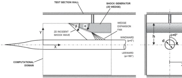
Figure 1. Schematic layout of experimental test setup with computational domain shown.
2. Methodology
2.1. Test case
The configuration of interest in this work was the sub-ject of a previous experimental investigation as reported by Brosh and Kussoy (1983). The configurations comprised a circular cylinder (d = 50.8 mm) of 1.016 m length (L), mounted centrally in a 0.254 m wide and 0.381 m high test section of a wind tunnel. The shock generator was a 2D wedge which was positioned above the cylinder at a distance of h/d = 2.97 from the top surface (Figure1).
The datum test flow conditions were M = 2.88,α = 16°, h = 150.9 mm, and a Reynolds number (ReL) of 18.2 × 10⁶ (Table 1) based on the free-stream velocity and length of the cylindrical body. This is the configura-tion for which the majority of the quantitative experimental data is available (Brosh & Kussoy,1983). The effect of the flow Reynolds number was also examined across the range of ReL = 7.28 × 10⁶to 58.3 × 10⁶, although for these configurations the free-stream Mach number also changed by modest amounts across the range of M = 2.8 to 2.95, respectively (Table1). The influence of the shock genera-tor angle (α) was further experimentally examined for an increased alpha of 19°, at the same Mach number (2.88) and Reynolds number (ReL= 18.2 ×10⁶) as the datum configuration and for a lower Reynolds number (ReL = 7.28 × 10⁶) with Mach number of 2.80 andαof 13°. The total temperature was kept relatively constant across the configurations and ranged between 101.4 K and 108.2 K.
Surface pressure taps were positioned on the cylinder at 20 mm axial intervals ( X/d = 0.39), with additional azimuthal taps at φ= 90°, 180° and 270° at 0.2 m axial spacing ( X/d = 3.9), to verify flow symmetry. Time-averaged static and total pressure profiles were measured in the windward (φ = 0°) and leeward (φ =180°) planes over a vertical distance from the surface of Y/d = 0.394 with a spatial resolution of Y/d = 9.8 × 10⁻⁴. It was assumed that total temperature was constant throughout the
Table 1. Brosh and Kussoy (1983) geometric and nom-inal flow conditions of tested computational models. Total Pressure T∞ α h ReL Mach PT∞(psi / kPa) (K) (deg.) (mm) (x106) No. 25 / 172.4 105.8 16 150.9 18.2 2.88 10 / 68.9 108.2 16 150.9 7.28 2.80 80 / 551.6 101.4 16 150.9 58.3 2.95 25 / 172.4 105.8 19 150.9 18.2 2.88
boundary layer in accordance with Kussoy, Horstman, and Acharya (1978). The reported measurement uncertainties in the windward and leeward planes were±10% for static pressure, ±1% for Pitot pressure, ±6% for static temper-ature, 12% for density, ±3% for velocity and ±1.97 × 10⁻³Y/d for the vertical probe movement in the Y-axis.
3. Computational model and method
The calculations were performed using Fluent V14.0 (SAS IP Inc., 2011a) using a steady, implicit density-based solver. The flow gradients were calculated using a least squares cell-based method with second order up-winding for the flow and turbulence properties. The convective fluxes are determined using the Roe flux difference split-ting scheme. For the turbulence models four eddy-viscosity models were selected; a one equation Spalart-Allmaras model, two equation k-εrealizable and k-ω SST models and a four equation k-ω SST model with a γ-θ transi-tion model (tSST). A seven equatransi-tion RSM model using the linear-pressure strain sub-model was also evaluated. For the fluid, specific heat capacity (Cp) was set via a three-coefficient polynomial temperature equation, Hilsenralh et al. (1955), which results inγ varying with temperature. Thermal conductivity was calculated by the use of kinetic-theory using the molecular and material properties of the fluid to account for the user defined Cp value. The three
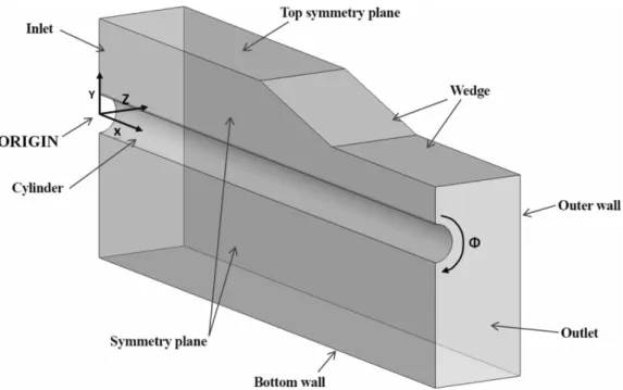
Figure 2. Model domain and boundary conditions.
coefficient method of Sutherland’s law, based on a refer-ence viscosity, temperature and effective temperature, was used to compute viscosity as a function of temperature. For all simulations, the double-precision solver was employed.
3.1. CFD domain and boundary conditions
The notation denotes ‘X’ as the axial axis, ‘Y’ as the vertical axis and ‘φ’ as the azimuthal direction around the cylinder and is shown in Figure2. The computational domain is also highlighted in Figure1. It comprises half the experimental domain, with the assumption of an X-Y sym-metry plane intersecting the cylinder atφ = 0°andφ = 180° to reduce the computational requirements. No-slip wall boundary conditions are defined for the wind tunnel walls, the wedge and the cylinder surfaces. A symmetry plane was used for the ‘top’ surface of the computation domain which was limited to the same vertical position as the top of, and prior to, the wedge to prevent artifi-cial boundary layer growth which could affect the shock wave characteristics. Experimental surface pressure data was limited axially, from X/d=1.97 to X/d = 16.34. The computational domain originates as shown in Figure2and extends axially X/d = 16.34, with the origin X/d = 7.83 upstream of the wedge leading edge.
At the inlet plane the total temperature, total pres-sure and Mach number are as specified in Table 1. As no information was provided on the turbulence charac-teristics in the wind-tunnel experiments, the values for turbulence intensity, I, and length scale, l, were determined from approximate empirical correlations based on ReDH
and the estimated boundary layer thickness ahead of the
shock impingement point, δ99 (Equations 1, 2) (SAS IP Inc., 2011b). The turbulence intensity, I, was 1.98% and the length scale,l/d, was 0.096.
I =0.16ReDH −1/8
(1)
l=0.4δ99 (2)
3.2. CFD grid
A structured multiblock approach was used with an O-grid blocking scheme around the cylinder with a radial expansion ratio of approximately 1.2 to grow the mesh and to provide between 40 and 90 cells across the boundary layer depending on the overall mesh resolution. The axial distribution of the mesh was clustered using an exponen-tial contraction in cell size up to the axial position of the wedge, aft of which uniform cell sizes were used.
Three grids of increasing resolution were generated; coarse, medium and fine with a refinement ratio of 1.5 in all three dimensions in accordance with the methodol-ogy outlined by Roache (1998). This yielded meshes of approximately 9×10⁵(900 k), 3 x10⁶ (3M) and 10×106 (10M) cells. To comply with turbulence models require-ments, a y+ less than 1 was maintained for all grids and test conditions.
The effect of the spatial discretisation was assessed using the generalized Richardson Extrapolation method (Celik et al.,2008). Grid Convergence Indices (GCIs) were assessed using nodal points of free-stream Mach number and total pressure ratio, PT/PT∞, at X/d = 9.84 on the windward surface, φ = 0°, of the cylinder. A factor of safety of 2 was used with the data showing the GCI to
be less than 1% for all cases and thus the grid was deter-mined as mesh insensitive according to the generalized Richardson Extrapolation. The characteristics of the gen-erated impinging shock was assessed using a position in between the wedge and the cylinder (Y/d = 1.56 and X/d= from 6.89 to 10.83). The static pressure and static temperature distributions in this region were evaluated rel-ative to the theoretical values and the effect of the grid resolution on these parameters was assessed. It was deter-mined that the static pressure and temperature ratios across the shock agreed to within ±1% of the theoretical value for the fine grid configuration.
3.3. Iterative convergence
Iterative convergence was assessed by considering the overall residual parameters throughout the flow domain in addition to integrated flow parameters. Overall, resid-uals were typically reduced to values below 10−4 for the continuity, momentum, energy and turbulence parameters. Due to the inherent unsteady nature of SBLIs and the assumption of ‘steady’ turbulence models, a simulation in which residual values below 10−4were maintained for 300 consecutive iterations was considered to have converged.
The convergence of flow characteristics at key loca-tions in the domain was monitored using a variety of met-rics. The windward static pressure at locations ahead of the shock impingement position (P1) and in the centre of the interaction (P2), were assessed. Within the accepted con-vergence tolerance, the reported values of static pressure at these locations varied by typically 0.2% and −1.6% for P1 and P2 respectively between initial stabilization at approximately 7000 iterations and the final converged value.
Integrated drag and moment coefficients for the full cylinder, Cdand Cm respectively, were also considered as part of the convergence assessment, and the parameters typically converged to stable values after 5000 iterations where the variation in Cd and Cm was 0.0005 and 0.0, respectively. A similar characteristic was also observed for y+ when averaged over the cylinder the variation with further iterations was in the order of 3.8%. The total mass averaged vorticity magnitude at the outlet plane was also considered and it was found to stabilize to within 1.5%.
For the cases with different Reynolds numbers (ReL, 7.28 × 10⁻⁶ and 58.3 × 10⁻⁶), the same domain as the datum configuration, with the 3M cell mesh, was used. For these cases, the y+ values over the whole cylinder were assessed and also found to be less than 1. For the config-uration where the shock generator wedge angle increased toα=19°, the geometry was slightly modified to accom-modate this change. However, the main parameters of the 3 million cell mesh were preserved to ensure the same number of cells across the boundary layer, overall mesh resolution and axial spacing in the main regions of interest.
Similarly the cylinder y+ was preserved at values less than 1.
4. Results
4.1. The datum configuration
The datum configuration was for a Mach number of 2.88, a ReLof 18.2×10⁶with a 16 degree wedge shock generator. The various turbulence models provide a range of results for the cylinder boundary layer at the position ahead of the SBLI. The boundary layer thickness (δ99) and compressible displacement thicknesses (δ*) is assessed at X/d =9.84 at
φ =0° where the boundary layer measurements showed a
δ99of 12.2 mm and aδ* of 3.5 mm, with uncertainties of ±3% and ±12.4%. The SST and tSST models calculated aδ99of 12.7 mm and 12.5 mm, respectively, with the latter being within the 3% experimental uncertainty range. The k-εand RSM models calculated a slightly thicker bound-ary layer withδ99 of +16.9% and +7.1%, respectively, relative to the measurements. However, the calculated dis-placement thicknesses showed a different sensitivity where the k-ε and RSM models provided δ* within the uncer-tainty level of -0.04 mm (-11.4%) and -0.04 mm (-12.3%), respectively. Conversely, the k-ω SST and γ-θ transi-tion k-ωSST models under-predictedδ* by approximately 30%.
The measurements of the surface static pressure ahead of the interaction indicate that there was a variation in the working section flow field conditions which is greater than the quoted uncertainty of the data acquisition system. Consequently, there are variations in the static pressure distributions on the cylinder ahead of the SBLI region, and therefore to enable a clear comparison of the pres-sure rise and SBLI extent for the CFD and experimental data sets, the cylinder surface static pressure has been nondimensionalized as shown in Equation (3):
P∗ PT,∞ ≡
Pw−Pref
PT,∞ (3)
where Pref is the average surface static pressure in the region ahead of the shock across the area between X/d = 2 and 5.5.
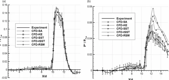
The surface static pressure distributions on the wind-ward (φ = 0°) and leeward (φ=180°) show notable differences in the characteristics of EV and RSM mod-els (Figure3). On the windward side, the pressure ratio, P*/PT∞, shows little difference between EV and RSM models and both are broadly in good agreement with the experimental results. Almost all of the data is within experimental uncertainty bounds although there are some key differences (Figure3). All models calculated a peak pressure ratio which is larger than the nominal exper-imental data with the SA, SST, tSST and k-ε models over-predicting the windward peak P*/PT∞ by approxi-mately 8.7%, 11.7%, 9.7%, and 9.6%, respectively. All
(a) (b)
Figure 3. (a) Windward (φ=0°) and (b) leeward (φ=180°) surface pressure plots comparing experimental and numerical results of EV and RSM turbulence models at every∼10thdata point. M=2.88,α=16°, ReL=18.2×10⁶, TT∞=278 K, PT∞=172.4 kPa.
of the models determine the position of the windward P*/PT∞ maximum to be at X/d = 10.61 which, within the spatial resolution, is in agreement with the experimen-tal location of X/d = 10.63. The nominal inviscid point of impingement of the shock is at X/d = 12.21 and, as expected, the SBLI results in a compression region ahead of this point. The experimental measurements indicate that the footprint is approximately 2.41 X/d upstream of the nominal impingement point with the major initial pressure rise occurring at X/d=9.84. Similarly, the k-ε, SST and tSST models all show evidence of this where the footprint is calculated to extend as far upstream as X/d = 9.80. There are small differences between the CFD models with the SA model exhibiting the rise further downstream at X/d =9.89 and the RSM model further upstream at X/d= 9.61. In the expansion region downstream of the local maximum there are no notable characteristic differences in the CFD results where all of the P*/PT∞ distributions are slightly higher than the measurements and generally at the upper limit of the measurement uncertainty. The experimental data indicates a small region of local re-compression at X/d = 11.5 which, although it is within the measurement uncertainty, is not reflected in any of the computations.
On the leeward side (φ = 180°), however, there are more notable differences between the CFD models as well as between the computational results and the measurements (Figure 3). Although all of the models broadly capture the locus of the initial pressure rise, there are large differences in the values of the local maxi-mum in P*/PT∞. In particular, peak values from the SA, SST and tSST models are 51%, 37% and 81% higher
than the measurements, respectively. Most of the pres-sure ratio distribution from the k-ε calculations were within the measurement uncertainty and the peak, P*/PT∞ was approximately 12% greater than the measurements. Finally, the best results were obtained using the RSM model where the pressure rise and peak value is within -8% of the measured value.
On the leeward side (Figure3), the measurements also clearly exhibit a double peak in P*/PT∞ due to a re-compression following the initial post-shock expansion with local maxima arising at X/d = 11.8 and 13.2. The SA, k-εand tSST models do not capture this recompres-sion. The SST and RSM simulations calculate this feature with the RSM getting the correct location, X/d =12.0 and 13.1, and the SST indicating that the local maxima are slightly further aft at X/d =12.1 and 13.6. The experi-ments indicate that the peak re-compression has a local relative magnitude of P*/PT∞=0.05. Although the SST and RSM models broadly capture the re-compression, the relative magnitude is around P*/PT∞= 0.065 and 0.04, respectively, or approximately +30% and -20% of the experimental values. Overall, based on the distributions of the surface P*/PT∞ ratio, the k-ε and RSM models provide the best agreement with the measurements with perhaps slightly better characteristics for the RSM where the additional modeling fidelity provides some very minor advantages in comparison with the more standard EV models.
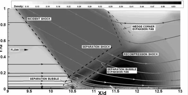
Figure 4illustrates the SBLI system in the windward side symmetry plane for the k-εcalculation using the 3M cell grid. The expected main flow features are evident such as the upstream separation shock, a following expansion
Figure 4. Calculated distribution of density on the windward side symmetry plane using the k-εmodel 3M mesh. M = 2.88,α=16°, ReL=18.2×10⁶, T
T∞= 278 K, PT∞= 172.4 kPa.
region, the primary reflected shock and a local region of boundary layer separation. The other models also resolved these main flow features. For this configuration, there is a boundary layer separation which, from the experimen-tal flow visualizations is estimated to extend from X/d = 10.1 to 10.7 along the cylinder symmetry plane. Both the EV and RSM models successfully calculate the occurrence of the separation region although with varying degrees of success. The SA model calculated a separated boundary layer region with an axial extent of 0.40 X/d which is approximately 31% shorter than that measured (0.58 X/d). For the other EV models, the k-ε, SST and tSST results showed separation lengths of X/d = 0.50, 0.55 and 0.60 which are approximately −12%, −4% and +5% differ-ent from the measuremdiffer-ents, respectively. The RSM model, however, provides the best calculation with a separation length of 0.58 X/d which is only -0.9% different from the measurements. This is a remarkably good level of agree-ment between the CFD and the experiagree-mental data given the complexity of the flowfield and is in disagreement with the over prediction of separation bubble size seen by Oliver et al. (2007). For the EV models, however, there is no clear relationship between the fidelity of the peak pressure ratio rise on the windward and leeward side and the accuracy of the calculation of the separation region length.
This SBLI is fundamentally three dimensional and the interaction is affected by the diffraction, and ultimate cross-ing, of the primary impinging shock around each side of the cylinder. These aspects result in a complex distribu-tion of the surface static pressure on the cylinder which is characterized by a predominantly quasi 2D pressure rise on the cylinder windward side, the sweep of the diffracted impinging shock and the notable subsequent local pres-sure rises on the leeward side due to the crossing of the
respective diffracted shocks. As also shown in the exper-imental results (Figure 5), the diffraction of the shock around the leeward side results in a region where the sur-face static pressure is affected by the impinging shock wave and its interaction with the curved cylinder surface. On the windward side the SBLI and pressure rise is affected by the local thickening of the boundary layer as well as the reflected shock. With increasing azimuthal angle the local pressure rise decreases as the shock reflection is reduced although this is a notable increase in the pressure rise again on the leeward side.
Where the shock interacts on the leeward side, it influ-ences the upstream flow conditions (Figure5), beginning experimentally at X/d= 11.0. By comparing this point of initial X/d Leeward Upstream Influence (LUI) in relation to the X/d position aft of the wedge, the CFD models can be compared. The X/d (LUI) position of the RSM model was effectively congruent with experimental data and within measurement uncertainty margins. The SA, k-ε, SST, and tSST EV models were +12.8%, 1.3%, 3.1%, and 4.7% respectively. The effect of the transition model was mod-est. The SA model again illustrated its inaccuracy for such SBLIs, whilst the tSST model was slightly worse than the SST model.
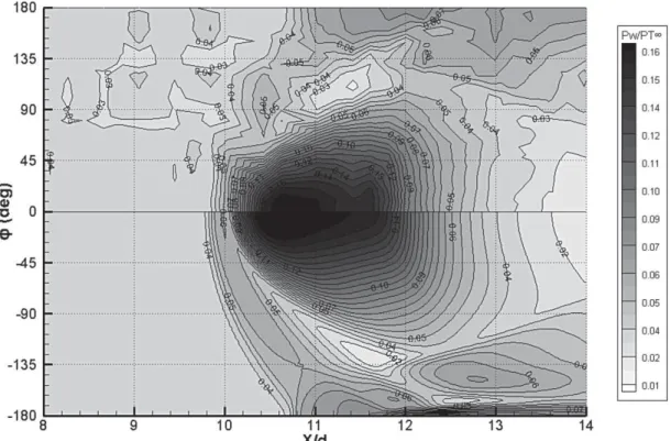
The distribution of p/PT∞over the cylinder highlights some of the aspects of the flow characteristics as the SBLI develops between the initial windward interaction (φ= 0°) and the eventual behavior on the leeward side. The measured distribution of p/PT∞ shows some of the main features although it is noteworthy that the resolution of the experimental data isφ =10° steps betweenφ= −10° to 190° (Figure5, Figure6). The spatial distribution along the cylinder surface (φ-X/d) highlights the main region of the strong SBLI pressure rise which is broadly concentrated
Figure 5. Comparison of experimental (top) and numerical (bottom) cylinder nondimensionalized surface pressure Pw/PT∞; SST model. 10M mesh. M= 2.88,α = 16°, ReL=18.2× 10⁶, TT∞= 278 K, PT∞= 172.4 kPa.
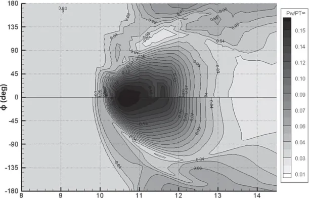
Figure 6. Comparison of experimental (top) and numerical (bottom) cylinder nondimensionalized surface pressure Pw/PT∞; RSM model. 10M mesh. M=2.88,α=16°, ReL=18.2×10⁶, T
T∞= 278 K, PT∞= 172.4 kPa.
(a) (b) (c) (d) (e) (f)
Figure 7. Comparison of computational streamlines, with experimental Mylar oil flow visualisation (a) SA, (b) k-ε, (c) SST, (d) tSST, (e) RSM. M=2.88,α=16°, ReL=18.2x10⁶, TT∞=278 K, PT∞=172.4 kPa.Figure 7(f): This figure is taken from NASA-TM-84410,
‘An Experimental Investigation of the Impingement of a Planer Shock Wave on an Axisymmetric Body at Mach 3’, by A. Brosh, M. Kussoy, and used with permission of NASA.
in the region of X/d=10 to 12 andφ from 0° to ±90°. The distributions of p/PT∞shows the reduction in p/PT∞ in the region aft of the main interaction as well as a region of relatively modest static pressure rise which borders the main shock interaction at around X/d = 11 to 12 and
φ = 90° to 135°. On the leeward side and the aft region (X/d =13 to 14), p/PT∞increases again. This is where the diffracted shock has propagated around the cylinder body, crosses the centerline and augments the static pressure due to the crossing with the diffracted shock from the opposite side. All of these main features are calculated by both the SST and the RSM models (Figure5, Figure6) and over-all there is good agreement in the topology of the surface static pressure distributions. In the leeward region there is a modest difference in the p/PT∞ distribution between the SST and RSM models where the SST shows regions with stronger rise and pressure gradients, particularly at
φ =140° andφ =180° (Figure5). The RSM model cal-culates more modest pressure gradients in this region and is in better agreement with the measurements (Figure5, Figure6).
As seen in the experiment, the computational results also show a strong lateral pressure gradient near the primary interaction at approximately X/d =10 to 11 (Figure5). This generates a strong crossflow and causes the flow to exhibit the wake type characteristics with sep-aration (Brosh & Kussoy, 1983). The measured location point of minimum pressure occurs atφ =110° and X/d = 11.4 (Figure 5). All of the eddy-viscosity models over-predict this azimuthal position of the minimum pressure point with the SA model having the largest difference
φ = 140° (+27%) although the other models also had notable differences, with k-ε, SST and tSST positions of
φ = 128° (+16%),φ = 132° (+20%), andφ = 135° (+23%), respectively. The RSM model provided the best results with the determined azimuthal position asφ=105° (−5%). The prediction of the lateral cross-flows was also in better agreement on the subsequent leeward side pres-sure field, with these distributions and prespres-sure gradients also affecting the local surface flow topology.
As part of the experimental studies, the surface flow topology was identified using a Mylar oil visualization method. This visualization highlighted the primary shock induced separation, which sweeps azimuthally around the cylinder, as well as the secondary separation line, notable crossflow regions and partial evidence of a tertiary separa-tion (Figure7).
The surface flow topology based on the skin friction distributions for the EV and RSM models are presented in Figure7. In the experiment the flow visualization indicates a strong cross flow region associated with the initial inter-action with the impinging shock which is also observed in all four eddy-viscosity models and best represented by the k-εmodel. All EV simulations, the first separation line, S1, and node of reattachment, NR1, seen in the experiment
are represented. The SA model, Figure7(a), captures the fewest aspects of the surface flow features with a secondary separation line, S2, as the only other main surface feature present. The k-εmodel, Figure 7(b), calculates a surface flow topology which is very similar to that of the SA model, and also fails to simulate the tertiary separation line. The SST, Figure7(c), and tSST, Figure7(d), models show similar primary features as with the SA and k-εmodels, but also include a tertiary separation line, S3, and are more like the experimental data. This tertiary separation is less clear in the SST model although a secondary attachment node, NR2, is present in both models and more clearly resolved in the SST model. The RSM model, Figure 7(e), shows the main features which are an improvement over the
k-εmodel. The SST model indicates a tertiary reattachment line (R3) in the region between X/d =12 to 13.5 although the transition model (Figure7(d)), shows a slightly differ-ent structure without a clearly defined R3. There is no clear evidence of such a feature in the flow visualization and overall the indications are that the RSM topology is more closely representative of the experimental data.
Overall it was found that for the RANS method, the turbulence model had a notable impact on the results. The turbulence model affected both the flow topology as well as the quantitative aspects of the SBLI. Of the EV models, the k-ω variants best represented the topology while the k-εmodels gave the best quantitative agreement. The SA model performed the worst and demonstrated its unsuit-ability for this type of SBLI. This conclusion has also been reached in the literature by Oliver et al. (2007), Bhag-wandin and DeSpirito (2011) and Tian and Lu (2013). The better agreement for the k-ε and k-ω formulations with experimental data, such as static surface pressures and sep-aration position, have been seen by Oliver et al. (2007) and Bhagwandin and DeSpirito (2011) when comparing two and three-dimensional SBLIs on flat plates and com-pression ramps. Three-dimensional work by DeBonis et al. (2010) of a shock impinging on a flat plate found that
k-ωmodels produced the lowest error when compared with SA, k-ε, k-ω and SST methods. The current work sup-ports these findings within the context of shock interactions on three-dimensional geometries in addition to highlight-ing improvements that are possible ushighlight-ing an RSM model when compared with the EV k-ε model. Vallet (2007) reported similar findings but for a simpler compression ramp configuration with varying incidence angles.
4.2. Effect of Reynolds number
The datum configuration was for a Reynolds number of 18.2 × 10⁶ with a freestream Mach number of 2.88. In the experiment, the effect of Reynolds number was consid-ered for values of 7.28 × 10⁶ and 58.3 ×10⁶ although in the experiment these also required a slight change in the freestream Mach number of 2.80 and 2.95, respectively
(a) (b)
Figure 8. (a) Windward (φ = 0°) and (b) leeward (φ=180°) surface pressure plots comparing k-εand RSM turbulence models at ReL = 58.3 ×10⁶compared to experimental data. Computational results show approximately every 10th data point. 3M mesh. M = 2.95,α = 16°, TT∞ = 278 K.
(a) (b)
Figure 9. (a) Windward (φ = 0°) and (b) leeward (φ = 180°) surface pressure plots comparing k-εand RSM turbulence models at ReL=7.28× 10⁶with datum CFD results (M = 2.88, Re
L=18.2 ×10⁶). Computational results show approximately every 10thdata point. 3M mesh. M=2.80,α =16°, TT∞= 278 K.
(Table 1). Although this therefore intertwines the effects of Reynolds number, shock strength and shock angle it is still of interest to investigate the changes in the SBLI and the ability of the CFD models to calculate these changes. As these configurations were not the main focus of the previous experimental study, there is a reduced amount of experimental measurements available for these configura-tions with surface pressure data and flow visualizaconfigura-tions for the higher Reynolds number (58.3 ×10⁶) case.
For the configuration with the Reynolds num-ber increased from the datum value of 18.2×10⁶ to 58.3×10⁶, the Mach number was also increased from
2.88 to 2.95 and therefore for a constant wedge angle of 16° there is a theoretical reduction in the shock angle from 34.2° to 33.6° and the static pressure ratio across the shock changes from 2.89 to 2.94. Overall these changes are relatively minor compared with the datum configura-tion (Figure 3) and both k-ε and RSM models produce results that are in close agreement with each other although neither captures the sudden drop in P*/PT∞at X/d=11.5 (Figure 8). On the leeward side, although there is some variation, the k-εshows better performance in terms of the peak pressure ratio rise (Figure8(b)) but the RSM shows the local pressure maximum at about X/d=13.5. The
Figure 10. Comparison of experimental (top) and numerical (bottom) cylinder nondimensionalized surface pressure Pw/PT∞; k-εmodel. 3M mesh. M = 2.95,α=16°, ReL=58.3×10⁶, TT∞= 278 K, PT∞= 551.6 kPa.
Figure 11. Comparison of experimental (top) and numerical (bottom) cylinder nondimensionalized surface pressure Pw/PT∞; RSM model. 3M mesh. M = 2.95,α = 16°, ReL= 58.3×10⁶, TT∞= 278 K, PT∞=551.6 kPa.
effect of reducing the Reynolds number from 18.2×10⁶ to 7.28×10⁶ was partially investigated in the experimen-tal work and computations of this lower Reynolds number case were also performed using the k-εand RSM models (Figure9). The calculations broadly show that there was
a slight increase in the strength of the interaction with the peak pressure rise on the windward side from the RSM cal-culations increasing from around 0.14 to 0.16 when ReL increased from 7.28 ×10⁶to 18.2×10⁶. The point of the initial pressure rise is slightly further upstream at the lower
(a) (b) (c) (d) (e) (f)
Figure 12. Comparison of computational streamlines, with experimental oil flow visualisation. Figures (a)–(c) M= 2.80,α=16°, ReL=7.28 ×10⁶, TT∞= 278 K, PT∞= 68.9 kPa. (a) k-ε, (b) RSM. Figures (d)–(f) M=2.95,α=16°, ReL= 58.3 ×10⁶, TT∞= 278 K, PT∞= 551.6 kPa. (d) k-ε, (e) RSM.Figure 12(c)(f): These figures are taken from NASA-TM-84410, “An Experimental
Investiga-tion of the Impingement of a Planer Shock Wave on an Axisymmetric Body at Mach 3,” by A. Brosh, M. Kussoy, and used with permission of NASA.
(a) (b)
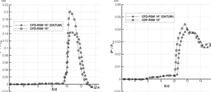
Figure 13. (a) Windward (φ=0°) and (b) leeward (φ=180°) surface pressure plot comparing k-εmodel atα=16° andα=19° at every∼10thdata point. 3M mesh. M=2.88, ReL=18.2×10⁶, TT∞=278 K, PT∞=172.4 kPa.
(a) (b)
Figure 14. (a) Windward (φ=0°) and (b) leeward (φ=180°) surface pressure plot comparing RSM model atα=16° andα=19° at every∼10thdata point. 3M mesh. M=2.88, Re
L=18.2×10⁶, TT∞=278 K, PT∞=172.4 kPa.
ReL, but this is within the uncertainty of the arrangement and the slight changes in the flow conditions. On the wind-ward side, the computations similarly show that the RSM model results in a lower peak pressure rise in comparison with the k-εresults. Concomitant with the slightly higher P*/PT∞on the windward side, both computations similarly show a slightly higher pressure rise on the leeward side.
The measured distributions of static pressure around the cylinder are shown in Figure10and Figure11for the high ReL of 58.3 × 10⁶ and compared with the results from the k-εand the RMS models. The point of minimum pressure for the high Reynolds case occurs experimen-tally at φ = 120°and X/d = 11.5. The EV and RSM models predict the minimum pressure position at X/d = 11.8,φ = 130° and X/d= 11.6,φ = 112°, respectively (Figure10 and Figure 11). In the low ReL case (ReL = 7.28 ×10⁶), the position of minimum pressure is found to be X/d=11.4 and 11.2,φ = 120° and 104° for EV and RSM models respectively. Whilst the axial positions are relatively close, the azimuthal positions vary more notably. In the datum simulations (Figure 5, Figure 6), the RSM model was found to calculate the axial position closer to the experimental results and this is borne out again for the high Reynolds case.
The impact of the change in ReLacross the range from 7.28×10⁶ to 58.3×10⁶ , for both the experimental flow visualizations as well as the k-ε and RSM computations is shown in Figure12. The differences in the flow topolo-gies are relatively minor and there is no notable change in either flow visualization of computational results. Nev-ertheless one of the notable features is in the separation bubble region at φ= 0° where the experiments indicate that the separation bubble is larger as ReLis reduced. This characteristic is also observed in both the k-ε and RSM results (Figure12(a,b,d,e)). For the RSM model there is
a slight change in the topology at the highest ReL (in Figure 12(e)), where there is evidence of a tertiary sepa-ration line starting at X/d = 13 and φ = 160°. Overall the numerical methods show similar levels of agreement with the experimental data at the increased Reynolds num-ber configuration and the RSM provides better agreement in the surface flow topology than the k-εsimulations.
4.3. Effect of shock strength
The results presented in section 5.1 above, indicate that for the datum configuration (M = 2.88,α= 16°, ReL= 18.2 × 10⁶) that the k-εand RSM methods provided the best agreement with the surface static pressures along the windward (φ = 0°) and leeward (φ = 180°) centerlines. In addition, the RSM model shows generally better agree-ment with the wider surface static pressure distributions and the overall flow topology. Although the experiment considered the impact of the shock strength on the interac-tion, by performing flow visualizations for a configuration where the wedge angle, α, was increased to 19°, the centerline pressure measurements were not acquired.
Nevertheless, given the confidence in the application of the k-εand RSM methods to this problem, it is of interest to assess the impact of the increase in the shock strength and change in incidence angle, on the simulated flow fields. The k-εand RSM methods both show similar changes in the centerline P*/PT∞(Figure13and Figure14) where the increase in shock strength from 0.14 to 0.20 for the RSM cases is broadly in agreement with the relative theoretical increase of 40% for an inviscid interaction. Of course, the overall levels of P*/ PT∞are lower than the inviscid value by approximately 30% based on the measurements for the datum configuration. Although the relative changes in P*/
(a) (b) (c) (c) (d) (e)
Figure 15. Comparison of computational streamlines, with experimental oil flow visualisation. Figures (a)-(c) M = 2.88,α =16°, ReL= 18.2 ×10⁶, TT∞= 278 K, PT∞= 172.4 kPa. (a) k-ε, (b) RSM. Figures (d)-(f) M = 2.88,α =19°, ReL= 18.2 × 10⁶, TT∞= 278 K, PT∞= 172.4 kPa. (d) k-ε, (e) RSM.Figure 15 (c)(f): These figures are taken from NASA-TM-84410, “An Experimental
Investigation of the Impingement of a Planer Shock Wave on an Axisymmetric Body at Mach 3,” by A. Brosh, M. Kussoy, and used with permission of NASA.
PT∞on the windward side are broadly as expected, on the leeward side the impact of the increased shock strength is attenuated through the interaction so that the increase in this region is only approximately 13% for both the k-εand RSM methods.
The increase in the impinging shock strength and change in shock angle has a small impact on the sur-face flow topology as illustrated in the flow visualizations (Figure15) but was more difficult to resolve computation-ally. This has been noted by Oliver et al. (2007) and DeBo-nis et al. (2010) with Vallet (2007) observing significant failures in the k-εmodel’s SBLI prediction ability at higher ramp incidence angles in comparison to RSM methods. The flow topology effects are likely due to the increased size of the separation bubble: when α is increased from 16° to 19°, there is a slight increase in the size of the pri-mary separation atφ = 0° and there are minor changes to the loci of the secondary and tertiary separation lines, S2 and S3, respectively. The k-ε model shows some of these characteristic changes, but the structure associated with the primary reattachment line (R1) and the absence of the tertiary separation (S3) indicates that the agreement with the experimental data is perhaps worse than the datum
configuration. As with the datum case, the RSM model shows better agreement with the oil visualization also for this case ofα =19°.
5. Conclusion
A shock–boundary layer interaction test case based on the complex configuration of planar oblique wave imping-ing onto the curved surface of a prismatic cylinder was computationally investigated. The investigation is based around an established test case under a nominal freestream Mach number of 2.88 and the impact of Reynolds number and shock strength and angle were also considered. The study assessed the performance of a range of computa-tional models and evaluated the results relative to quan-titative experimental data as well as flow visualizations. The research considered a range of eddy viscosity RANS models including the Spalart-Allmaras, k-εRealisable,
k-ωShear Stress Transport and the k-ωSST model with a
γ-θtransition model. In addition a Reynolds Stress Model was also evaluated. A computational approach was devel-oped to establish mesh independence as well as appropriate iterative convergence.