QUANTIFYING THE EFFECTS OF VARIABLE SELECTION, SPATIAL SCALE AND SPATIAL DATA QUALITY IN MARINE BENTHIC HABITAT MAPPING
by
© Vincent Lecours A Thesis submitted to the School of Graduate Studies
in partial fulfillment of the requirements for the degree of
Doctor of Philosophy Department of Geography Memorial University of Newfoundland
September 2016 St. John’s
ii
Abstract
Mapping benthic habitats has become critical in many contexts like conservation and management. While marine habitat mapping methods strongly rely on tools and methods from geography and geomatics, habitat mapping practitioners with a background outside of these specialized areas do not always have a full understanding of the spatial concepts behind these tools and methods. This phenomenon is amplified when marine geomorphometry, the science used to quantify seafloor terrain characteristics, is integrated into the marine habitat mapping workflow. This dissertation reviews the use of spatial concepts in the field of marine benthic habitat mapping; many concepts are poorly understood or poorly implemented in the habitat mapping workflow, among which spatial scale and spatial data quality stand out as being of particular importance.
While geomorphometry is commonly used in marine benthic habitat mapping, no framework existed to test which terrain attributes should be used as surrogates of species distribution, leading to an inability to compare results from different studies. This dissertation explores different options for terrain attribute selection and proposes an optimal combination that can be used as standard in all habitat mapping studies. This selection is then tested using two approaches to benthic habitat mapping and is shown to perform better than others.
Bathymetric data, the primary input for marine geomorphometry analyses and one of the main data inputs for habitat mapping, are commonly impacted by data acquisition artefacts. Very little work has been done on trying to understand how these artefacts propagate throughout the habitat mapping workflow. The impact of artefacts on the
iii
bathymetry and its derived terrain attributes is described, and it is shown that artefacts modify the spatial and statistical distributions of depth and terrain attribute values. However, when these affected data are used in habitat mapping, their impact is not always predictable. Some artefacts were found to sometimes inflate measures of accuracy and performance and sometimes decrease them.
Overall, habitat maps were shown to be very sensitive to the effects of variable selection, spatial scale and data quality, and as such have serious implications when they are used to inform decision-making, for instance in marine conservation and management. This dissertation raises awareness about these issues and highlights the need for careful integration of spatial data in habitat mapping practices.
iv
Co-Authorship Statement
This dissertation is written in manuscript style with the goal of publishing Chapters 2 to 6. The author of this dissertation has been the primary researcher behind the work performed in each of the chapters, including developing the ideas, reviewing the literature, designing the experiments, analyzing the data, interpreting the results, and preparing the manuscripts. The co-authors and committee members have contributed ideas, assisted in the development of the different methods and the interpretation of results, and reviewed the manuscripts. In terms of the manuscripts, the author of this dissertation is the primary author on all the manuscripts included in this dissertation. The co-authors contributed by critically reading and providing feedback on the different manuscripts.
Chapter 2, “Spatial Scale and Geographic Context in Benthic Habitat Mapping: Review and Future Directions” was published in 2015 in the journal Marine Ecology Progress Series (vol. 535, p. 259-284). This manuscript was written in close coordination with co-supervisor Dr. Rodolphe Devillers (Department of Geography, Memorial University), and with the help of Dr. David Schneider (Department of Ocean Sciences, Memorial University). Committee members Dr. Vanessa Lucieer (Institute for Marine and Antarctic Studies, University of Tasmania) and Dr. Craig Brown (Nova Scotia Community College), and co-supervisor Dr. Evan Edinger (Department of Geography, Memorial University) provided feedback on versions of this manuscript.
Chapter 3, “Towards a Framework for Terrain Attribute Selection in Environmental Studies”, has been submitted to the journal Environmental Modelling & Software in June
v
2016 and is currently under review. The analysis performed in this manuscript was supervised by Dr. Devillers and Dr. Alvin Simms (Department of Geography, Memorial University). Dr. Devillers, Dr. Simms, and committee members Dr. Lucieer and Dr. Brown provided feedback on versions of this manuscript.
Chapter 4, “Comparing Selections of Environmental Variables for Ecological Studies: A Focus on Terrain Attributes”, has been submitted to the journal PLoS One in June 2016 and is currently under review. Dr. Brown and Dr. Devillers supervised the development of the methods, and provided feedback on versions of the manuscript, together with Drs. Lucieer and Edinger.
Chapters 5 and 6 were written for submission to a journal after completion of this dissertation. Drs. Devillers, Lucieer and Brown provided feedback on versions of Chapter 5, and Drs. Devillers and Edinger provided feedback on versions of Chapter 6.
Other publications led by the author are not presented in this dissertation but were part of the author’s PhD work. A short book chapter and a full-length review article of the field of marine geomorphometry, an important component of this dissertation, were published. Preliminary results from Chapter 3, gained using slightly different methods from those in Chapter 3, were also published as a short book chapter. In terms of spatial data quality, an evaluation of uncertainty propagation to bathymetric data collected from a remotely operated vehicle in the deep sea was published in conference proceedings. A technical report that explored benthic habitat mapping methods to study cold-water coral habitats at multiple scales using geomorphometry was also presented to the Department of Fisheries and Oceans Canada. Finally, a short paper looking at the application of a new
vi
algorithm for photo-mosaicking images of the seafloor to habitat mapping was published in Sea Technology. The relevant references are listed below.
Lecours, V., Dolan, M.F.J., Micallef, A., & Lucieer, V. (2016) A review of marine geomorphometry, the quantitative study of the seafloor. Hydrology and Earth System Sciences, 20:3207-3244.
Lecours, V., Lucieer, V.L., Dolan, M.F.J., & Micallef, A. (2015) An ocean of possibilities: applications and challenges of marine geomorphometry. In: Jasiewicz, J., Zwolinski, Z., Mitasova, H., & Hengl, T. (Eds) Geomorphometry for geosciences. BoguckiWydawnictwoNaukowe,Poznan, Poland, p. 23–26.
Lecours, V., Simms, A., Devillers, R., Lucieer, V. & Edinger, E. (2015) Finding the best combinations of terrain attributes and GIS software for meaningful analysis. In: Jasiewicz, J., Zwolinski, Z., Mitasova, H., & Hengl, T. (Eds) Geomorphometry for geosciences.BoguckiWydawnictwoNaukowe,Poznan, Poland, p. 133-136.
Lecours, V., & Devillers, R. (2015) Assessing the spatial data quality paradox in the deep-sea. In: Sieber, R.E. (Ed.) Proceedings of Spatial Knowledge and Information Canada, 2015:1–8.
Lecours, V., Miles, L.L., Devillers, R., & Edinger, E.N. (2013) Data analysis towards the multiscale characterization of cold-water coral and sponge habitats in Canadianwaters. Technical Report REQ. No. F6160-120010. Department of Fisheries and Oceans Canada, Newfoundland and Labrador Region, St. John’s, 260 p.
Bagheri, H., & Lecours, V. (2012) Benthic habitat mapping using high-resolution image mosaicking. Sea Technology, 53:15-20.
vii
Acknowledgements
The journey to completing this dissertation was shaped by all the individuals who I encountered in the last few years and who have given me time, expertise, financial and moral support. I have grown professionally and personally in the last five years, and these people have definitely contributed to that growth.
First and foremost, I would like to acknowledge my supervisors Rodolphe Devillers and Evan Edinger, who have been there for me every time I needed, whether it was work-related or otherwise. They provided guidance, expertise and financial support, but I am most grateful for all the opportunities they gave me to learn and experience throughout my degree. They understand that a PhD is not just a piece of paper they give you at the end of a long and arduous journey, but it is actually a training that involves interactions with others as much as analyses. Whether it was for conferences, workshops, professional meetings, teaching opportunities, or allowing me to go get lost on a boat in the middle of the Pacific Ocean with other scientists, they were always supportive, and that means a lot to me. I am very grateful for their trust in me and the independence they gave me.
Many thanks to my research committee, Craig Brown and Vanessa Lucieer, for their insightful comments and discussions on my research and for dealing with my tendency to always do more (or too much…). Thanks are also due to David Schneider, Alvin Simms, Marie-Josée Fortin, Margaret Dolan, and Aaron Micallef who contributed directly to my work, and to all the others that I contacted throughout the years for advice or help on topics related to my research. Also, thanks to Trevor Bell, Chris McGonigle and Eric Vander Wal for reviewing my dissertation and providing useful comments on it.
viii
My gratitude also goes to the Geography Department at Memorial University. The faculty, students, and staff have made my time in the department unforgettable. I am thankful to have been part of such a great group in the Marine Geomatics Research Lab and the Marine Habitat Mapping Research Group. To all alumni, current students, postdocs and visiting researchers with whom I shared more than just a working space, thanks for tolerating my occasional grumpiness. Arnaud and Daniel deserve special mention for the freshly-made coffee every morning.
I am grateful to all the organizations that provided funding for my research or for conferences: the Natural Sciences and Engineering Research Council of Canada (NSERC), the School of Graduate Studies of Memorial University, the Department of Fisheries and Oceans Canada, the Office of the Vice-President (Research) of Memorial University, the Canadian Foundation for Innovation (CFI), the Atlantic Division of the Canadian Association of Geographers, the Department of Geography of Memorial University, GeoHab and Esri Canada.
Finally, thanks to my friends, in Québec, Newfoundland and elsewhere, who supported, encouraged and most importantly entertained me throughout this whole thing. Thanks to Emma, who has been more than patient with me, listening and providing me with daily, unconditional support (and food!). Thanks to my parents, who encouraged me to jump into this adventure, my sister who showed me the example, and to my grand-parents and aunts who are always happy to hear about what I am doing, even if they do not always understand much!
ix
Table of Contents
Abstract ... ii Co-Authorship Statement ... iv Acknowledgements ... vii Table of Contents ... ixList of Tables ... xiii
List of Figures ... xiv
List of Abbreviations ... xvii
List of Appendices ... xix
1. Introduction and Overview ... 1
1.1 Introduction ... 1
1.2 Research Problem and Research Gap ... 6
1.3 Research Questions ... 8
1.4 Research Hypotheses ... 9
1.5 Research Objectives ... 10
1.6 Methods ... 11
1.7 Significance of Research ... 12
1.8 Organization of the Dissertation ... 13
1.9 Literature Cited ... 14
2. Spatial Scale and Geographic Context in Benthic Habitat Mapping: Review and Future Directions ... 20
2.1 Introduction ... 20
2.2 Scale in Ecology ... 24
2.3 Scale in Benthic Habitat Mapping ... 29
2.3.1 Review of Concepts and Methods ... 29
2.3.1.1 Habitat Mapping ... 29
2.3.1.2 Surrogacy ... 33
2.3.1.3 Species Distribution Modelling ... 34
2.3.2 Ecological Scale: Benthic Species and Their Environment... 36
2.3.2.1 Environmental and Biological Surrogates ... 36
2.3.2.2 Combined Environmental Influence and Multicollinearity ... 37
2.3.3 Observational Scale: Representing Nature with Spatial Data ... 39
2.3.3.1 Adequacy of Spatial Data ... 39
2.3.3.2 Data Quality and Spatial Scale ... 41
2.3.4 Analysis Scale: Influence on Analyzing Ecogeographical Data ... 43
2.3.5 Multiscale and Multi-Design Approaches ... 44
2.3.5.1 Multiple Scales and the MAUP ... 44
2.3.5.2 Multiscale and Multi-Design Frameworks ... 46
2.3.5.3 Studying Benthic Habitats at Multiple Scales ... 47
2.4 Adding Geographic Context by Considering the Spatial Nature of Data ... 48
2.4.1 Spatial Autocorrelation ... 49
2.4.2 Using Spatial Statistics to Account for Spatial Heterogeneity ... 52
2.5 Future Directions – Integrating Spatial Concepts in Habitat Mapping ... 54
2.5.1 Past, Current and Future Trends in Benthic Habitat Mapping ... 54
x
2.5.3 Recommendations ... 62
2.6 Conclusions ... 63
2.7 Literature Cited ... 65
3. Towards a Framework for Terrain Attribute Selection in Environmental Studies ... 94
3.1 Introduction ... 94
3.2 Materials and Methods ... 97
3.2.1 Surfaces and Terrain Attributes ... 99
3.2.1.1 Artificial Surfaces ... 99
3.2.1.2 Terrain Attributes and GIS Tools ... 101
3.2.1.3 Preparation of the Data ... 101
3.2.2 Principal Component Analysis ... 102
3.2.2.1 Identifying the Optimal Number of Components ... 103
3.2.2.2 Complexity of Variables ... 103
3.2.2.3 Towards a Final Solution ... 104
3.2.2.4 Validation ... 104
3.2.2.5 Comparisons ... 105
3.2.2.6 Interpretation ... 105
3.2.3 Multicollinearity assessment: variable inflation factor and mutual information 106 3.3 Results ... 107
3.3.1 Terrain Attributes and Software ... 107
3.3.2 Principal Component Analysis ... 108
3.3.2.1 Number of Components, Variance and Communality ... 108
3.3.2.2 Configuration ... 108
3.3.2.3 Complexity of Variables ... 112
3.3.3 Variable Inflation Factor and Mutual Information ... 113
3.4 Discussion ... 114
3.4.1 Surface Complexity and Importance of Terrain Attributes ... 114
3.4.2 Terrain Attributes, Algorithms and Software ... 115
3.4.3 Suitable Subset of Terrain Attributes ... 117
3.5 Conclusion ... 119
3.6 Literature Cited ... 121
4. Comparing Selections of Environmental Variables for Ecological Studies: a Focus on Terrain Attributes... 128
4.1 Introduction ... 128
4.2 Materials and Methods ... 129
4.2.1 Data ... 130
4.2.2 Unsupervised Classifications of Potential Habitat Types ... 134
4.2.3 Supervised Classifications of Sea Scallop Habitats ... 135
4.3 Results ... 137
4.3.1 Unsupervised Classifications ... 137
4.3.1.1 Performance of Classifications ... 137
4.3.1.2 Discrimination of Benthoscape Classes ... 140
4.3.1.3 Spatial Variations of Outputs from Different Selections ... 141
4.3.2 Supervised Classifications ... 142
4.3.2.1 Predictive Capacity and Robustness... 142
4.3.2.2 Generalizability ... 144
xi
4.3.2.4 Spatial Variations of Predictions from Different Selections ... 147
4.4 Discussion ... 147
4.4.1 Framework for Terrain Attribute Selection ... 147
4.4.2 Selections of Terrain Attributes ... 148
4.4.3 Terrain Morphology as an Environmental Factor ... 149
4.4.4 Consequences of Variable Selection ... 151
4.4.5 Comparisons with Other Studies: Terrestrial and Marine ... 152
4.5 Conclusion ... 153
4.6 Literature Cited ... 154
5. A Multiscale Analysis of the Impact of Artefacts in Multibeam Bathymetric Data on Terrain Attributes... 158
5.1 Introduction ... 158
5.2 Material and Methods ... 162
5.2.1 Data ... 162
5.2.2 Comparisons ... 168
5.3 Results and Interpretation ... 172
5.3.1 Reference Surfaces (No Artefact) ... 172
5.3.2 Altered Surfaces ... 175
5.3.2.1 Artefacts ... 176
5.3.2.2 Bathymetry and Terrain Attributes... 179
5.3.2.3 Spatial Scale ... 180
5.4 Discussion ... 182
5.4.1 Comparisons with Other Studies: Terrestrial and Marine ... 182
5.4.2 Implications for Marine Geomorphometry ... 185
5.5 Conclusions ... 190
5.6 Literature Cited ... 192
6. Influence of Artefacts in Digital Terrain Models on Habitat Maps and Species Distribution Models: A Multiscale Assessment ... 201
6.1 Introduction ... 201
6.2 Material and Methods ... 204
6.2.1 Case Study and Data ... 204
6.2.2 Habitat Maps and SDMs ... 207
6.3 Results ... 210
6.3.1 Habitat Maps ... 210
6.3.1.1 Reference Habitat Maps ... 210
6.3.1.2 Habitat Maps from Altered Data ... 211
6.3.2 Species Distribution Models ... 216
6.3.2.1 Reference SDMs ... 216
6.3.2.2 SDMs from Altered Data ... 219
6.4 Discussion ... 226
6.4.1 Reference Habitat Maps and SDMs ... 226
6.4.2 Impacts of Artefacts on Habitat Maps and SDMs ... 230
6.4.3 Spatial Errors in the Ecological Literature ... 233
6.4.4 Implications for Ecological Applications ... 235
6.5 Conclusions ... 238
6.6 Literature Cited ... 239
7. Conclusion ... 250
xii
7.1.1 Findings ... 251
7.1.2 Research Hypotheses ... 254
7.2 Research Contributions and Highlights ... 256
7.3 Future Directions ... 258
7.3.1 Limitations and Future Opportunities ... 258
7.3.2 Emerging Questions ... 260
7.3.3 Recommendations for Marine Habitat Mapping Practices ... 261
7.4 Conclusions ... 264
xiii
List of Tables
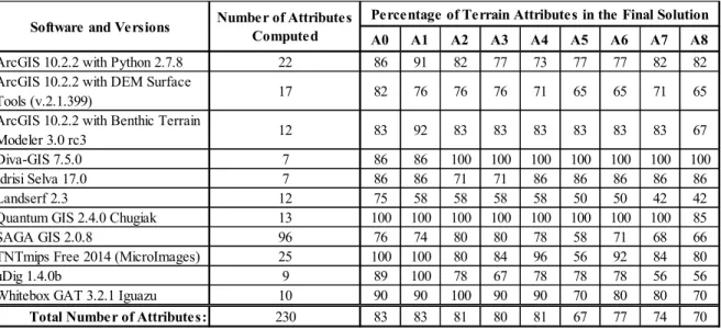
Table 3.1: List of software used, number of terrain attributes that were computed using each of them, and percentage of these terrain attributes that reached the final PCA solution for each surface. ... 101 Table 3.2: Percentage of the 230 variables that formed each solution or were removed during the
iterative PCA. Complex variables that loaded equally on more than one component were removed, while complex variables that loaded more strongly on one component were kept (Appendix A)... 113 Table 4.1: Selections of terrain attributes used to build the habitat maps and models. The ID
numbers refer to Lecours et al. (submitted) and allow finding the software and parameters with which the attributes were generated. Marker variables correspond to important
variables; whether they were found on strong components (Sel. 1) or weak components (Sel. 4) is linked to the amount of topographic structure they accounted for. Variables with low cardinality (Sel. 2) did not have many different values, thus limiting their ability to explain slight variations in terrain morphology. Complex variables (Sel. 3) correspond to redundant variables. ... 133 Table 4.2: Spatial similarity of the habitat maps and SDMs generated from Selections 2 to 7,
compared to the map and model built from Selection 1. A similarity of 90% indicates that 90% of the pixels were classified as the same habitat type in the two compared maps, or that 90% of the pixels were within ±5% of probability distribution in the two compared models. ... 141 Table 5.1: Statistics of the range of motion recorded during the surveys, and levels of artefact
induced to the five reference DBMs. Statistics for time values are based on the five
calibration values used by the CHS. The sign convention used is positive pitch with the bow up and positive roll with the port side up. ... 167 Table 5.2: Comparison of the characteristics of the shallower (A in Figure 5.1) and the deeper (B
in Figure 5.1) sub-areas. ... 168 Table 5.3: Change in statistical distribution of values with coarsening scales, based on linear
regressions. Grey cells indicate non-significant relationships (assessed with the F statistic). White cells indicate significant relationship; the sign in them indicates whether the equations had a positive or negative slope. ... 174 Table 6.1: Levels of artefacts introduced in the five reference DBMs. Standard deviations (σ)
were derived from the recorded motion at time of survey. A positive pitch indicates that the bow is up and a positive roll means that the port side is up. ... 206 Table 6.2: Mean and standard deviation of kappa coefficients of agreement of the ten maps made
from altered data for each type of artefact, each scenario and each scale. ... 212
xiv
List of Figures
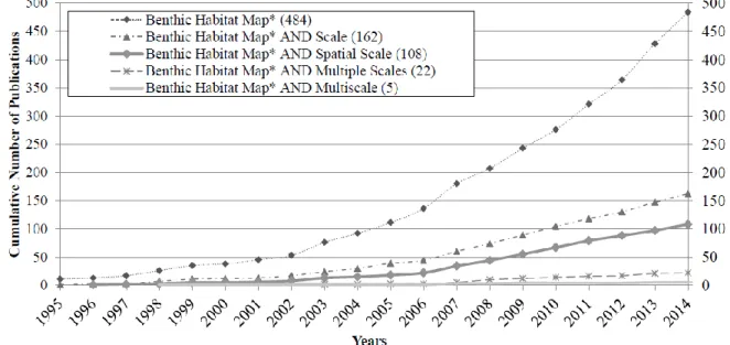
Figure 2.1: Cumulative number of publications (articles or reviews) listed in the Scopus database mentioning specific keywords (see key) in their title, abstract or keywords, by the end of 2014. ... 23 Figure 2.2: Seabed profiles (black lines) showing fine-scale (solid gray ellipses),
intermediate-scale (dashed gray ellipses) and broad-intermediate-scale (dotted gray ellipses) topographic features delineated using (A) finer-scale and (B) coarser-scale bathymetric data. By using only a coarse observational scale, information on potentially ecologically important finer-scale features is not captured. (Conceptual figure shows bathymetric profiles derived from the General Bathymetric Chart of the Oceans [GEBCO] dataset; www.gebco.net/). ... 40 Figure 2.3: (A) Multiscale and (B) multi-design continuum-based approaches. Both extent and
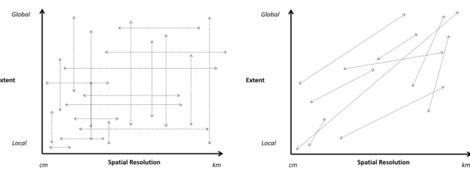
resolution vary in a multi-design approach, while only one of these 2 scale characteristics is modified in a multiscale survey; each dotted line illustrates an example of how a single study could be framed. ... 47 Figure 2.4: Conceptual representation of the implementation of a continuum-based multiscale
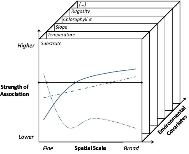
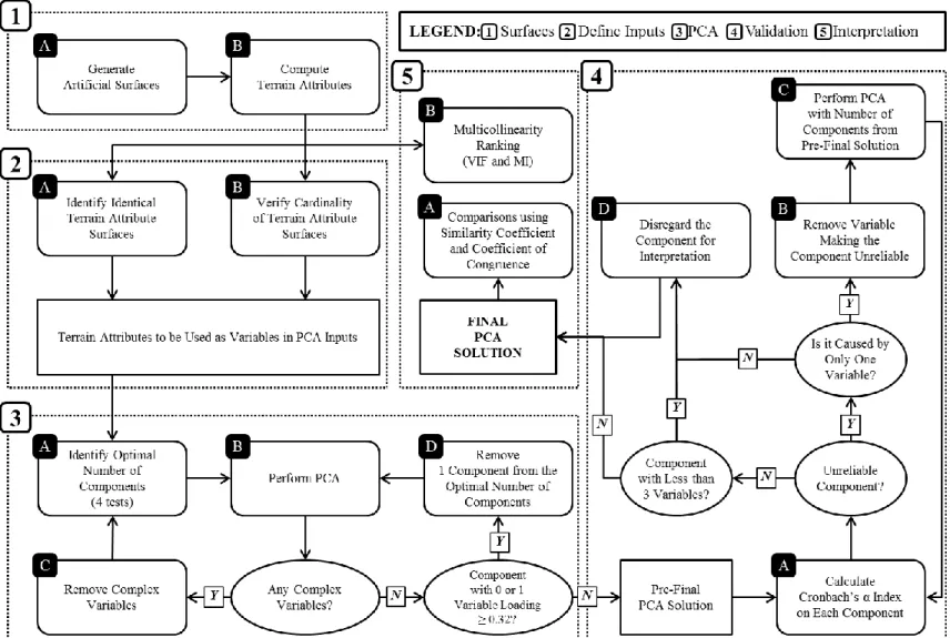
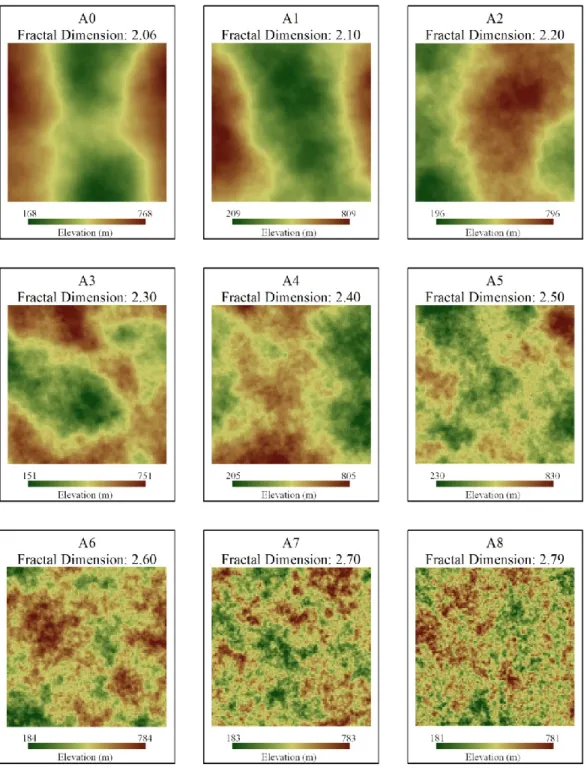
approach to explore scale-dependency of species-environment relationships. By sampling several environmental characteristics (z axis) at multiple spatial scales (x axis), it is possible to quantify the strength of association (y axis) between a species and its habitat as a function of scale (blue curves). The black horizontal line represents a given significance threshold. Note that if a coefficient of correlation was to be used to measure significance, there would be 2 significance thresholds: one for strongly positive correlations and one for strongly negative correlations. Curves are hypothetical and inspired by results from Horne & Schneider (1997) (pelagic species), and Schneider et al. (1987) and Kendall et al. (2011) (benthic and epibenthic species)... 57 Figure 3.1: Conceptual model of the analysis performed on each artificial surface. ... 98 Figure 3.2: Artificial surfaces computed and analyzed in this study, from least complex (A0) to
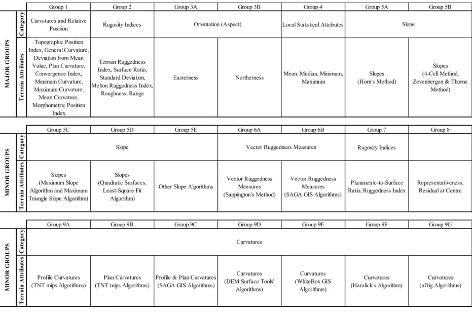
most complex (A8). ... 100 Figure 3.3: Main groups of multicollinear terrain attributes that consistently loaded together on
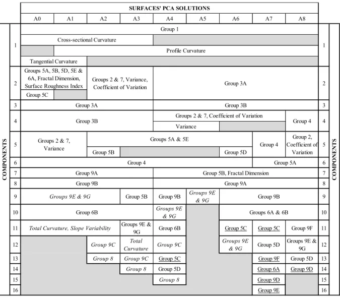
the different components. ... 110 Figure 3.4: Summary of the PCA solutions' configuration. The different groups are detailed in
Figure 3.3. Characters in italic represent the unreliable components as assessed by
Cronbach's α, and underlined characters indicate components with less than three variables. ... 111 Figure 4.1: German Bank study area with some of the input variables used in this study: the
ground-truth data for the bottom types, the sea scallops observations, the bathymetry, the three backscatter derivatives and the six terrain attributes from Selection 1. ... 131 Figure 4.2: Map accuracies measured with (A) a kappa coefficient of agreement and (B) the
overall accuracy. ... 139 Figure 4.3: Performance and robustness of the 29 MaxEnt models. Models in the top-left corner
xv
Selection 2 (blue), Selection 3 (red), Selection 4 (green), Selection 5 (purple), Selection 6 (orange), Selection 7 (white). ... 143 Figure 4.4: Generalizability of the 29 MaxEnt models. Models closer to the top-left corner are
more generalizable as they performed well on the training data and replicated well to the validation data. See Figure 4.3 for colour legend. ... 145 Figure 5.1: 50 m resolution DBM of German Bank (top) with its six terrain attributes derived
(bottom). Two specific sub-areas, one in shallower waters (A) and one in deeper waters (B), were used in the analyses and are indicated by a black square in the main map... 164 Figure 5.2: The reference panels to the left show the bathymetry and terrain attributes of the
shallower sub-area (2.5 km by 2.5 km; same colour scheme as Figure 5.1). The panels to the right show examples of error (absolute difference between the reference and altered
surfaces) for that sub-area. The level of error represented is the highest one (5σ, Table 5.1). Numbers in the right margins indicate error ranges (note differences in scales). Colours range from yellow (lowest) to red (highest). ... 170 Figure 5.3: The reference panels to the left show the bathymetry and terrain attributes of the
deeper sub-area (2.5 km by 2.5 km; same colour scheme as Figure 5.1). The panels to the right show examples of error (absolute difference between the reference and altered surfaces) for that sub-area. The level of error represented is the highest one (5σ, Table 5.1). Numbers in the right margins indicate error ranges (note differences in scales). Colours range from yellow (lowest) to red (highest). ... 171 Figure 5.4: Correlations between the 10 m resolution surfaces and the same surfaces computed at
different scales. For instance, the 50 m topographic position surface of the full study area is correlated at about 0.10 with the 10 m topographic position surface of the full area. ... 173 Figure 6.1: Digital Bathymetric Model of the German Bank study area. ... 206 Figure 6.2: Kappa coefficients of agreement and overall accuracies of the 15 reference habitat
maps. ... 210 Figure 6.3: Kappa coefficients of agreement of the 615 habitat maps. ... 213 Figure 6.4: Examples of habitat maps produced with 8 layers at 50 m resolution, overlaid by the
ground-truth data. The level of error represented in the lower maps is the highest one (5σ, Table 6.1). ... 214 Figure 6.5: Spatial distribution of the change in habitat map classification between the maps
presented in the bottom of Figure 6.4 and the reference map shown on top of Figure 6.4. 215 Figure 6.6: Number of habitat maps made from altered bathymetric and terrain attribute data that
had a higher kappa coefficient of agreement than the reference habitat maps. No habitat maps impacted by roll performed better than the reference maps. ... 216 Figure 6.7: Performance and robustness (left) and generalizability (right) of the 15 reference
MaxEnt models. Models are colour-coded following Figure 6.3: dark blue (10 m resolution), red (25 m), green (50 m), purple (75 m) and light blue (100 m). High AUCTest values
indicate that models performed well on validation data and low standard deviations indicate robust models. High AUCTrain values indicate that models performed well on training data
and low AUCDiff indicate that they replicated well on validation data. In both graph, the best
xvi
Figure 6.8: A) Spatial correlation between the reference MaxEnt models for the three scenarios and their corresponding reference models at other scales (e.g. the models computed with 7 layers at 50 m and 10 m have a r value of 0.85). B) Spatial correlation between the reference models of different scenarios at each scale (e.g. models computed at 50 m resolution with 7 and 8 layers have a r value slightly above 0.70)... 219 Figure 6.9: Change in performance and robustness as the level of artefacts in the data changes.
The blue symbols are the reference models. The darker a symbol, the greater the level of artefact is. Green indicates positive artefact alterations (e.g. positive pitch) while red indicate negative alterations (Table 6.1). High AUCTest indicate that models performed well and low
standard deviations indicate robust models. Good and robust models are located in the Northwest quadrant. ... 221 Figure 6.10: Differences in probability distribution between models affected by artefacts and a
reference model (top). The scenario represented is the one with 8 layers at 50 m resolution. The level of error represented is the highest one (5σ, Table 6.1). ... 222 Figure 6.11: Generalizability of all SDMs as the level of artefacts in the data changes. High
AUCTrain indicate that models performed well on training data and low AUCDiff indicate that
they replicated well on validation data. More generalizable models are thus located in the Northwest quadrant. See Figure 6.9 for legend. ... 224 Figure 6.12: Spatial variation in predictions of sea scallops distribution as quantified by the range
in correlation coefficients between models built from altered data and the reference models. ... 226
xvii
List of Abbreviations
AUC Area Under the CurveAUV Autonomous Underwater Vehicle CC Coefficient of Congruence
CHS Canadian Hydrographic Service COS Change-Of-Support
DBM Digital Bathymetric Model DEM Digital Elevation Model
DFO Department of Fisheries and Oceans Canada DTM Digital Terrain Model
GEBCO General Bathymetric Chart of the Oceans GIS Geographic Information System
GPS Global Positioning System
GWR Geographically Weighted Regression
ICES International Council for the Exploration of the Sea IID Independent and Identically Distributed
IMU Inertial Measurement Unit LiDAR Light Detection and Ranging
MAP Minimum Average Partial Correlation MAUP Modifiable Areal Unit Problem MaxEnt Maximum Entropy
xviii
MESH Mapping European Seabed Habitats MI Minimum Information
MIM Minimum Information Matrix MMU Minimum Mapping Unit PA Parallel Analysis
PCA Principal Components Analysis RDMV Relative difference to Mean Value ROC Receiver Operating Characteristic ROV Remotely Operated Vehicle SAC Spatial Autocorrelation SC Similarity Coefficient
SCUBA Self-Contained Underwater Breathing Apparatus SDM Species Distribution Model
SWATH Small Waterplane Area Twin Hull
TASSE Terrain Attribute Selection for Spatial Ecology TPI Topographic Position Index
VIF Variable Inflation Factor VRM Variable Ruggedness Measure
xix
List of Appendices
Appendix A Detailed Material and Methods (Chapter 3)………265 Appendix B Artificial Surfaces and List of Derived Terrain Attributes, with Software,
Algorithms, References, and Duplicates (Chapter 3)………..273 Appendix C Extended Results of the Iterative Principal Component Analysis (PCA),
Variable Inflation Factor (VIF), and Mutual Information (MI), for all Surfaces and Derived Terrain Attributes (Chapter 3)……….286 Appendix D Additional Information on Maps and Models Performance (Chapter 4).344 Appendix E Detailed Results (Chapter 5)………346 Appendix F Overall Accuracies of the Habitat Maps (Chapter 6) ……….375
1. Introduction and Overview
1.1IntroductionWhile the oceans are estimated to comprise up to 90% of the inhabitable area for life on Earth (Tittensor et al., 2009), and despite over 150 years of exploration, the scientific community still knows very little about the marine environment compared to its terrestrial counterpart (Roberts, 2002). Historically, knowledge about the marine environment was often gained and driven by human use of the oceans, partly through the exploitation of natural resources. For instance, the presence of cold-water corals has been documented by fishermen since the mid-eighteenth century (Roberts, 2002), and more recently coral observations from fisheries bycatch have helped describe their presence, abundance and geographic distribution (Cogswell et al., 2009; Murillo et al., 2011). The realization in the twentieth century that the oceans, especially in the deep sea, are not muddy and lifeless triggered interest in documenting more than just species occurrences by mapping marine habitats. Marine habitat mapping then became a scientific endeavour, often an applied one designed to answer specific scientific and management questions. For instance, marine habitat mapping has been used to inform conservation efforts (e.g. Laffoley & Hiscock, 1993; Light, 1998), to study juvenile mortality in benthic invertebrates (e.g. Gosselin & Qian, 1997), to study the disturbance of seabed habitats from fishing gear (e.g. Friedlander et al., 1999), and to evaluate ecological associations between different species (e.g. Olsgard et al., 2003).
In the last 25 years, the importance of anthropogenic pressure on seafloor environments and the growing realization of the significance of these ecosystems, for
instance in terms of ecosystem services (Galparsoro et al., 2014), have steered many nations towards increasing efforts to better manage and protect marine resources (Borja, 2014). Such efforts led scientists to define standards for marine habitat mapping, and many definitions of benthic habitats were proposed (e.g. Kostylev et al., 2001; Harris & Baker, 2012). In its simplest form, a benthic habitat is a distinct area of the seafloor characterized by a combination of specific chemical, physical and/or biological characteristics. Mapping the seafloor based on species’ habitat requirements has become critical in many contexts, and is often the first step in implementing scientific management, monitoring environmental change, and assessing the impacts of anthropogenic disturbance on benthic ecosystems (Roff et al. 2003; Cogan & Noji 2007). Seafloor mapping also provides the data necessary for the identification and monitoring of marine protected areas (Le Pape et al., 2014). Habitat maps enable the interpretation of the nature, distribution, and extent of distinct physical environments, and allow predictions of species or communities distribution based on their associations with the environment (Harris and Baker, 2012).
The field of marine benthic habitat mapping has evolved rapidly during these 25 years. Technological and methodological developments in marine benthic habitat mapping were partly driven by innovations in geomatics, more specifically in Geographic Information Systems (GIS), spatial analysis methods and remote sensing technologies (Wright & Heyman, 2008; Brown et al., 2011). In their “Review of Standards and Protocols for Seabed Habitat Mapping”, Coggan et al. (2007) defined a very general approach to marine benthic habitat mapping as the spatial integration of different datasets,
usually within a geospatial environment. Within a GIS environment, spatial analytical techniques are combined with high-resolution geoscientific and environmental data with in situ observations to enable accurate quantification and representation of habitats. This provides a framework for mapping the distribution of benthic species and interpreting spatial patterns in biodiversity (Whitmire et al., 2007; Brown et al., 2011; Harris and Baker, 2012). For a long time, habitat mapping was done using available, often broad-scale data. For instance, while bycatch data and bathymetric data from satellite radar altimetry provide some understanding of species biogeography at a regional scale (e.g. Bryan & Metaxas, 2007), they present challenges when trying to understand habitat characteristics at a more local scale that is often more meaningful for purposes such as conservation and management (Etnoyer & Morgan, 2007). However, the development of acoustic remote sensing and bathymetric LiDAR techniques in recent decades has helped fill the gap in high-resolution spatial environmental data necessary to map benthic habitats at scales relevant to such purposes. Data provided by this type of remote sensing, specifically bathymetry and backscatter data, have revolutionized benthic habitat mapping, both in terms of the methods used and our ability to map habitats efficiently and with relative ease. Bathymetric and backscatter data are used for seafloor characterization, habitat mapping, and the derivation of surrogates to predict species distribution (Butler et al., 2006; Anderson et al., 2008; Dolan et al., 2008). These data have proven their value for habitat mapping and their potential to help the scientific community advance its understanding of seafloor ecosystems (Anderson et al., 2008; Brown et al., 2011).
Like benthic habitat mapping, geomorphometry – the science used to derive quantitative measurements of terrain characteristics from digital terrain models (DTM) – has been fueled by advances in remote sensing and GIS in recent decades (Florinsky, 2012) and now strongly rely on methods and techniques from geomatics. Geomorphometry has traditionally focused on the investigation of terrestrial landscapes, but the dramatic increase in the availability of digital bathymetric data and the increasing ease by which geomorphometry can be analyzed using GIS has prompted interest in employing geomorphometric techniques to investigate the marine environment (e.g. Lundblad et al., 2006; Wilson et al., 2007). Over the last decade or so, a multitude of geomorphometric techniques have been applied to characterize the seafloor, and marine benthic habitat mapping is a major area where the use of marine geomorphometry has grown in recent years (reviewed in Lecours et al., 2016). Linked to the increasing use of multibeam and bathymetric LiDAR data for benthic habitat mapping (Brown et al., 2011; Smith and McConnaughey, 2016), the vast majority of habitat mapping studies with access to bathymetric data are now using, or at least testing, some form of terrain attributes (e.g. slope, orientation, rugosity) in their workflow. Since most marine habitats are difficult to access, observe and sample (Solan et al., 2003; Robinson et al., 2011), bathymetric data are often the only reliable dataset available to characterize benthic habitats; by enabling the extraction of quantitative information from bathymetric data, geomorphometry provides an invaluable source of additional and relevant information for benthic habitat mapping.
In the context of marine geomorphometry, the roles of several spatial concepts are still not studied (e.g. spatial data quality) or fully understood (e.g. spatial scale), and these spatial concepts are often overlooked when marine geomorphometric techniques are used in marine benthic habitat mapping. By its spatial and data-driven natures and the near ubiquitous use of GIS, remote sensing and spatial analysis in its workflow, marine habitat mapping and its practices are also directly influenced by spatial concepts such as spatial scale and spatial autocorrelation. However, the scientists framing the questions related to the study of benthic habitats and the managers applying the answers are frequently not trained in the geomatics tools that underpin much of the new techniques in marine habitat mapping. While geographers and other spatial scientists have been studying these fundamental concepts for a long time, the understanding of their role and their integration in the habitat mapping workflow – including during geomorphometric analyses – have received scant attention in the past. Since marine habitat maps have become a critical tool in decision-making, especially in marine conservation and management (Reiss et al., 2014; Buhl-Mortensen et al., 2015; Davies et al., 2015; Rolet et al., 2015; Howell et al., 2016), there is an urgent need to improve our understanding of how these concepts influence the representation of benthic ecosystems and habitats. This dissertation focuses on marine benthic habitat mapping methods, and particularly on how a better integration of spatial concepts like spatial scale can improve the marine habitat mapping workflow. It is aimed at developing best practices in the application of geomatics-based marine habitat mapping to ecological and management questions. A particular focus is given to the concepts of variable selection, spatial scale and spatial data quality.
1.2 Research Problem and Research Gap
The general problem that this dissertation addresses is that of a widely used but poorly understood spatial framework for marine benthic habitat mapping research. Some work has been done (e.g. Dolan et al., 2008; Brown et al., 2011; Rengstorf et al., 2012; Dolan & Lucieer, 2014; Rattray et al., 2014) to improve our understanding of the influence of certain spatial concepts (e.g. spatial scale, spatial data quality) on the way we represent and understand benthic habitat. However, much work remains to be done to enable the full integration or consideration of spatial concepts within the habitat mapping workflow. This problem is rooted in the disconnection between marine habitat mapping – a field that is spatial in nature – and the field of geomatics, which provides the spatial concepts that partly support many habitat mapping practices. Geomatics is intrinsically linked to geography and is defined as the “discipline dedicated to the management of spatially referenced data, and thus relies on the scientific concepts and technologies implied in the acquisition, storage, analysis, and distribution of the data” (Caron et al., 2008, p. 295).
Through the development of GIS, which offer tools to analyze and represent spatial data, geomatics has become very accessible to a wide range of scientists involved in marine benthic habitat mapping (e.g. geologists, ecologists, biologists). The effectiveness of geomatics concepts and methods – and of GIS tools to assist in the exploration of questions from other disciplines – has given rise to the multidisciplinary and interdisciplinary nature of the field (Wright et al., 1997; Mark, 2000, 2003; Blaschke et al., 2011, 2012). First, these concepts and tools enable a better understanding of complex
phenomena by integrating information in a spatial context, and incorporating both qualitative and quantitative spatial reasoning with concepts from other disciplines (e.g. geology or ecology) into a common framework. Then, geomatics provides a set of core concepts that improve communication and mutual understanding about spatial data and information among researchers with different backgrounds (Kuhn, 2012). As a consequence, geomatics has been widely adopted by many disciplines in the last 25 years (Raper, 2009; Blaschke & Merschdorf, 2014), including geomorphometry (Zhou & Zhu, 2013) and marine habitat mapping (Wright & Heyman, 2008).
Geomatics is an integrative science. As Lam & Kemp (2012, p. 2194) stated: “Integrative science is the cornerstone of this field – both helping others integrate and integrating other sciences into ours to see where the technology and science are lacking.” Geomatics is thus considered a multiparadigmatic science in which approaches from other disciplines are commonly applied within the field, and vice-versa (Blaschke and Merschdof, 2014). However, the integrative nature of geomatics also has downsides. The development of easily accessible tools brings hidden dangers by facilitating non-critical use by end-users (e.g. computer scientists, ecologists, geologists) who may have limited appreciation of spatial concepts, for instance spatial scale, spatial representation and spatial data quality. Because the tools are made to be intuitive, they often do not require end-users to fully understand the characteristics of the underlying processes and parameters implemented in the tools, and of the spatial data that form the basis for analysis. The scientific concepts and foundations are thus often hidden behind increasingly “black-box”, user-friendly tools. In addition, the fast pace at which tools and
techniques are developing may commonly prevent end-users from remaining apprised of new developments in these scientific concepts and foundations. This leads to the danger of inappropriate use of geospatial data and tools and the lack of appropriate consideration of important spatial concepts, from which misinformed and potentially erroneous interpretations or inferences could be made.
In summary, there is a lack of consideration, likely caused by a lack of understanding, of spatial concepts (e.g. spatial scale, spatial data quality, spatial autocorrelation) within marine benthic habitat mapping practices. There is a need to reunite the community of end-users – e.g. the geologists, ecologists, geographers, or decision-makers involved in the production of benthic habitat maps – with the spatial foundations that underpin the data, tools and methods they use. The specific research gap that this dissertation addresses is the following: there are currently no best practices defined to better integrate spatial concepts like spatial scale and spatial data quality in the marine benthic habitat mapping workflow, particularly when marine geomorphometric analyses are part of this workflow.
1.3 Research Questions
The research problem can be addressed by increasing geographic literacy in disciplines like marine habitat mapping and marine geomorphometry that commonly use spatial data and GIS tools (Blaschke & Strobl, 2010).This dissertation attempts to answer the following questions to increase the body of knowledge related to spatial concepts in marine benthic habitat mapping, and more particularly on spatial scale and spatial data quality. Since marine geomorphometry is an important part of the marine habitat mapping
workflow, these questions will be answered through the integration of geomorphometric analyses in the habitat mapping practices.
1. Which particular spatial concepts are poorly integrated in the marine benthic habitat mapping workflow, and is it possible to identify specific ways to improve the integration of spatial concepts in marine benthic habitat mapping?
2. Which combination of terrain attributes best capture seafloor characteristics while minimizing spatial covariation? Can these terrain attributes form a standard protocol for using marine geomorphometry in different approaches to habitat mapping?
3. How sensitive are these terrain attributes to different types of data acquisition artefacts? Does the sensitivity of terrain attributes to data acquisition artefacts vary with spatial scale?
4. Do data acquisition artefacts propagate to habitat maps and species distribution models? Are the impacts of data acquisition artefacts on habitat maps and species distribution models scale-dependent?
1.4 Research Hypotheses
The following five hypotheses are examined in this dissertation:
1. There is a lack of understanding of the role of different spatial concepts, for instance like spatial scale and spatial data quality, in marine benthic habitat mapping practices.
2. Different optimal combinations of terrain attributes exist and their composition varies depending on seafloor characteristics (e.g. roughness).
3. The different optimal combinations of terrain attributes are generalizable, i.e. they can be integrated in the marine habitat mapping workflow regardless of the approach used to map habitats.
4. Terrain attributes, and habitat maps and species distribution models produced from these terrain attributes, are sensitive to data acquisition artefacts.
5. The sensitivity of terrain attributes, habitat maps and species distribution models to data acquisition artefacts is scale-dependent; finer-scale data, and maps and models built from these data, are more sensitive to data acquisition artefacts than broader-scale data and maps and models produced with these data.
1.5 Research Objectives
The overarching objective of this dissertation is to identify spatial concepts that currently lack a proper consideration in marine benthic habitat mapping practices, and to propose solutions towards a better (re)integration of these concepts into the marine benthic habitat mapping workflow. A particular focus is given to spatial scale, spatial covariation, and spatial data quality.
Specific objectives are:
1. Review existing knowledge on spatial concepts in benthic habitats and their mapping, including the related practices of surrogacy assessment and species distribution modelling.
2. Identify ways to improve marine benthic habitat mapping practices through a better integration of spatial concepts.
3. Identify combinations of environmental variables that minimize spatial covariation and optimize the information extracted from these data.
4. Demonstrate the importance of using spatial data with an ecological meaning for marine benthic habitat mapping by describing the effects of subjectively selecting spatial data on the production of habitat maps and species distribution models. 5. Describe the impacts of a poor spatial data quality on the marine benthic habitat
mapping workflow.
6. Evaluate the relationship between spatial scale and spatial data quality in a marine benthic habitat mapping context.
1.6 Methods
Through its exploration of the role of spatial concepts in marine benthic habitat mapping, this dissertation focuses on one specific type of spatial data: bathymetry. Since it often is the only reliable continuous dataset available to characterize benthic habitats, particularly in deeper waters, bathymetry has become the most important dataset in marine benthic habitat mapping. By definition, bathymetry is the representation of the seafloor that defines the benthic component of benthic habitats. Bathymetry is also the primary input to geomorphometric analyses. Based on this, this dissertation focuses on the integration of spatial concepts in marine benthic habitat mapping when marine geomorphometry practices are also integrated in the workflow. While the dissertation addresses many spatial concepts, including spatial autocorrelation and spatial heterogeneity, it focuses on issues related to spatial scale, spatial data quality, and spatial
covariation among environmental variables like terrain attributes that are commonly used in marine habitat mapping.
This dissertation is based on the evaluation of different practices and methods related to the production of benthic habitat maps. Consequently, it often necessitated a control dataset on which hypotheses could be tested. Two main datasets were used in this dissertation. The first one includes nine artificial terrain surfaces that provided a controlled environment for defining a framework for the use of marine geomorphometry in marine benthic habitat mapping (cf. Chapter 3). The second dataset is that of the German Bank, an area off Nova Scotia that has been extensively studied before (e.g. DFO, 2006; Todd et al., 2012; Brown et al., 2012). This dataset include bathymetry, backscatter data, and two types of ground-truth data (photographs of the seafloor and biological observations). This dataset is an excellent example of complete dataset that can be found in the literature, and enabled controlling variables for testing hypotheses in Chapter 4, Chapter 5, and Chapter 6. Its previous uses also provide opportunities for comparison of methods and results.
1.7 Significance of Research
By demonstrating the impacts of an inappropriate integration of spatial concepts in the marine benthic habitat mapping workflow, this dissertation will increase awareness amongst habitat mapping practitioners of the importance to consider these concepts. This should lead to an increased geographic literacy within marine habitat mapping. It should also result in more tools being developed and made accessible through GIS to a wide range of marine scientists, which should facilitate the integration of spatial concepts in the
workflow and eventually improve standards and protocols. Ultimately, an increased realization amongst the community of the importance of spatial concepts should lead to a change in practices, which will enable the production of knowledge on benthic habitats grounded on a sound, spatially-explicit inferential basis. Consequently, such knowledge will better support decisions made from habitat maps in contexts such as conservation and management. Finally, this dissertation also defines standards for the use of geomorphometry in marine habitat mapping, which now provide an operational framework for habitat mapping practitioners willing to integrate geomorphometric analyses in their workflow. The adoption of that framework by the community will now enable valid comparisons between studies.
1.8 Organization of the Dissertation
This dissertation is organized into seven sections: the introduction, five manuscripts, and a conclusion chapter.
Chapter 2 reviews the marine benthic habitat mapping literature and highlights the importance of incorporating ecological scaling and geographical theories in this field. Recommendations are provided on more effective practices for marine benthic habitat mapping.
Chapter 3 focuses on the use of terrain attributes derived from DTMs. An optimal combination of terrain attributes for use in marine benthic habitat mapping was proposed after testing 230 tools and algorithms on nine artificial surfaces.
Chapter 4 uses the recommended selection of terrain attributes from Chapter 3 – defined in a theoretical context – in a practical context of marine benthic habitat mapping.
It demonstrates the selection’s superiority over others in the production of marine habitat maps and species distribution models.
Chapter 5 addresses spatial data quality at multiple spatial scales. It describes how different types of data acquisition artefacts that are common in multibeam bathymetric data impact the derivation of terrain attributes from bathymetry.
Chapter 6 pushes forward the analyses from Chapter 5 by exploring how the artefacts errors propagate to habitat maps and species distribution models when bathymetry and terrain attributes are used in their production.
In Chapter 7 the relevance and implications of this research is discussed within the context of marine benthic habitat mapping but also in a wider context of ecological and marine research. Future research areas that can build upon this research but are beyond the scope of this dissertation are also discussed.
1.9 Literature Cited
Anderson, J.T., Holliday, D.V., Kloser, R., Reid, D.G., & Simard Y. (2008) Acoustic seabed classification: current practice and future directions. ICES Journal of Marine Science, 65:1004-1011.
Blaschke, T., & Merschdorf, H. (2014) Geographic information science as a multidisciplinary and multiparadigmatic field. Cartography and Geographic Information Science, 41:196-213.
Blaschke, T., & Strobl, J. (2010) Geographic Information Science Developments. GIS.Science Zeitschrift für Geoinformatik, 23:9-15.
Blaschke, T., Strobl, J., & Donert, K. (2011) Geographic information science: building a doctoral programme integrating interdisciplinary concepts and methods. Procedia – Social and Behavioral Sciences, 21:139-146.
Blaschke, T., Strobl, J., Schrott, L., Marschallinger, R., Neubauer, F., Koch, A., Beinat, E., Heistracher, T., Reich, S., Leitner, M., & Donert, K. (2012) Geographic information science as a common cause for interdisciplinary research. In: Gensel, J., Josselin, D., & Vandenbroucke, D. (Eds) Bridging the Geographic Information Sciences, Springer Lecture Notes in Geoinformation and Cartography. Berlin: Springer, pp. 411-427.
Borja, A. (2014) Grand challenges in marine ecosystems ecology. Frontiers in Marine Science, 1:1-6.
Brown, C.J., Sameoto, J.A., & Smith, S.J. (2012) Multiple methods, maps, and management applications: purpose made seafloor maps in support of ocean management. Journal of Sea Research, 72:1-13.
Brown, C.J., Smith, S.J., Lawton, P., & Anderson, J.T. (2011) Benthic habitat mapping: a review of progress towards improved understanding of the spatial ecology of the seafloor using acoustic techniques. Estuarine, Coastal and Shelf Science, 92:502-520.
Bryan, T.L., & Metaxas, A. (2007) Predicting suitable habitat for deep-water gorgonian corals on the Altantic and Pacific continental margins of North America. Marine Ecology Progress Series, 330:113-126.
Buhl-Mortensen, L., Buhl-Mortensen, P., Dolan, M.F.J., & Gonzalez-Mirelis, G. (2015) Habitat mapping as a tool for conservation and sustainable use of marine resources: some perspectives from the MAREANO Programme, Norway. Journal of Sea Research, 100:46-61.
Butler, J., Neuman, M., Pinkard, D., Kvitek, R., & Cochrane, G. (2006) The use of multibeam sonar mapping techniques to refine population estimates of the endangered white abalone (Haliotis sorenseni). Fishery Bulletin, 104:521-532.
Caron, C., Roche, S., Goyer, D., & Jaton, A. (2008) GIScience journal ranking and evaluation: an international Delphi study. Transaction in GIS, 12:293-321.
Cogan, C.B., & Noji, T.T. (2007) Marine classification, mapping, and biodiversity analysis. In: Todd, B.J., & Greene, H.G. (Eds) Mapping the seafloor for habitat characterization, Geological Association of Canada, Special Paper 47, pp. 129-139.
Coggan, R., Populis, J., White, J., Sheehan, K., Fitzpatrick, F., & Piel, S. (2007) Review of standards and protocols for seabed habitat mapping, 2nd edition. MESH (Mapping European Seabed Habitats). www.emodnet-seabedhabitats.eu/default.aspx?page=1442.
Cogswell, A.T., Kenchington, E.L.R., Lirette, C.G., MacIsaac, K., Best, M.M., Beazley, L.I., & Vickers, J. (2009) The current state of knowledge concerning the distribution of coral in the Maritimes Provinces. DFO Canadian Technical Report of Fisheries and Aquatic Sciences, 2885, 66 p.
Davies, J.S., Stewart, H.A., Narayanaswamy, B.E., Jacobs, C., Spicer, J., Golding, N., & Howell, K.L. (2015) Benthic assemblages of the Anton Dohrn Seamount (NE Atlantic): Defining deep-sea biotopes to support habitat mapping and management efforts with a focus on vulnerable marine ecosystems. PLoS ONE, 10:e0124815.
DFO (2006) Presentation and review of Southwest Nova Scotia benthic mapping project. DFO Canadian Science Advisory Secretariat, Proceedings Series 2006/047.
Dolan, M.F.J., Grehan, A.J., Guinan, J.C., & Brown, C. (2008) Modelling the local distribution of cold-water corals in relation to bathymetric variables: adding spatial context to deep-sea video data. Deep-Sea Research I, 55:1564-1579.
Dolan, M.F.J., & Lucieer, V.L. (2014) Variation and uncertainty in bathymetric slope calculations using geographic information systems. Marine Geodesy, 37:187-219.
Etnoyer, P., & Morgan, L.E. (2007) Predictive habitat model for deep gorgonian needs better resolution: comment on Bryan & Metaxas (2007). Marine Ecology Progress Series, 339:311-312.
Florinsky, I.V. (2012) Digital terrain analysis in soil science and geology. Elsevier/Academic Press, The Netherlands, 379 p.
Friedlander, A.M., Boehlert, G.W., Field, M.E., Mason, J.E., Gardner, J.V., & Dartnell, P. (1999) Sidescan-sonar mapping of benthic trawl marks on the shelf and slope off Eureka, California. Fishery Bulletin, 97:786-801.
Galparsoro, I., Borja, A., & Uyarra, M.C. (2014) Mapping ecosystem services provided by benthic habitats in the European North Atlantic Ocean. Frontiers in Marine Science, 1:23-36.
Gosselin, L.A., & Qian, P.Y. (1997) Juvenile mortality in benthic marine invertebrates. Marine Ecology Progress Series, 146:265-282.
Harris, P.T., & Baker, E.K. (2012) Seafloor geomorphology as benthic habitat: GeoHab atlas of seafloor geomorphic features and benthic habitats. Elsevier, Amsterdam.
Howell, K.-L., Piechaud, N., Downie, A.-L., & Kenny, A. (2016) The distribution of deep-sea sponge aggregations in the North Atlantic and implications for their effective spatial management. Deep-Sea Research Part I, 115:203-220.
Kostylev, V.E., Todd, B.J., Fader, G.B.J., Courtney, R.C., Cameron, G.D.M., & Pickrill, R.A. (2001) Benthic habitat mapping on the Scotian Shelf based on multibeam bathymetry, surficial geology and sea floor photographs. Marine Ecology Progress Series, 219:121-137.
Kuhn, W. (2012) Core concepts of spatial information for transdisciplinary research. International Journal of Geographical Information Systems. 26:2267-2276.
Laffoley, D., & Hiscock, K. (1993) The classification of benthic estuarine communities for nature conservation in Great Britain. Netherland Journal of Aquatic Ecology, 27:181-187. Lam, N.S., & Kemp, K.K. (2012) Reflections on Geographic Information Science: special
issue in honor of Michael Goodchild. International Journal of Geographical Information Science, 26:2193-2196.
Lecours, V., Dolan, M.F.J., Micallef, A., & Lucieer, V. (2016) A review of marine geomorphometry, the quantitative study of the seafloor. Hydrology and Earth System Sciences, 20:3207-3244.
Le Pape, O., Delavenne, J., & Vaz, S. (2014) Quantitative mapping of fish habitat: a useful tool to design spatialised management measures and marine protected area with fishery objectives. Ocean & Coastal Management, 87:8-19.
Light, J.M. (1998) Marine molluscan conservation: the value of mapping as a conservation tool. Journal of Conchology, special issue, 147-154.
Lundblad, E., Wright, D.J., Miller, J., Larkin, E.M., Rinehart, R., Naar, D.F., Donahue, B.T., Anderson, S.M., & Battista, T. (2006) A benthic classification scheme for American Samoa. Marine Geodesy, 29:89-111.
Mark, D.M. (2000) Geographic information science: critical issues in an emerging cross-disciplinary research domain. Journal of the Urban and Regional Information Systems Association, 12:45-54.
Mark, D.M. (2003) Geographic information science: defining the field. In: Duckham, M., Goodchild, M.F. & Worboys, M.F. (Eds) Foundations of Geographic Information Science. London: Taylor & Francis, pp. 3-18.
Murillo, F.J., Munoz, P.D., Altuna, A., & Serrano, A. (2011) Distribution of deep-water corals of the Flemish Cap, Flemish Pass, and the Grand Banks of Newfoundland (Northwest Atlantic Ocean): interaction with fishing activities. ICES Journal of Marine Science, 68:319-332.
Olsgard, F., Brattegard, T., & Holthe, T. (2003) Polychaetes as surrogates for marine biodiversity: lower taxonomic resolution and indicator groups. Biodiversity & Conservation, 12:1033-1049.
Raper, J. (2009) Geographical information science. In: Cronin, B. (Ed.) Annual Review of Information and Science and Technology.
Rattray, A., Ierodiaconou, D., Monk, J., Laurenson, L.J.B., & Kennedy, P. (2014) Quantification of spatial and thematic uncertainty in the application of underwater video for benthic habitat mapping. Marine Geodesy, 37:315-336.
Reiss, H., Birchenough, S. Borja, A., Buhl-Mortensen, L., Craeymeersch, J., Dannheim, J., Darr, A., Galparsoro, I., Gogina, M., Neumann, H., Populus, J., Rengstorf, A.M., Valle, M., Hoey, G.V., Zettler, M.L., & Degraer, S. (2014) Benthos distribution modeling and its relevance for marine ecosystem management. ICES Journal of Marine Science, 72:297-315.
Rengstorf, A.M., Grehan, A., Yesson, C., & Brown, C. (2012) Towards high-resolution habitat suitability modeling of vulnerable marine ecosystems in the deep-sea: resolving terrain attribute dependencies. Marine Geodesy, 35:343-361.
Roberts, C.M. (2002) Deep impact: the rising toll of fishing in the deep sea. TRENDS in Ecology & Evolution, 17:242-245.
Robinson, L.M., Elith, J., Hobday, A.J., Pearson, R.G., Kendall, B.E., Possingham, H.P., & Richardson, A.J. (2011) Pushing the limits in marine species distribution modelling: lessons from the land present challenges and opportunities. Global Ecology and Biogeography, 20:789-802.
Roff, J.C., Taylor, M.E., & Laughren, J. (2003) Geophysical approaches to the classification, delineation and monitoring of marine habitats and their communities. Aquatic Conservation, 13:77-90.
Rolet, C., Spilmont, N., Dewarumez, J.-M., & Luczak, C. (2015) Linking macrobenthic communities structure and zonation patterns on sandy shores: mapping tool toward
management and conservation perspectives in Northern France. Continental Shelf Research, 99:12-25.
Smith, T.A., & McConnaughey, R.A. (2016) The applicability of sonars for habitat mapping: a bibliography. U.S. Department of Commerce, NOAA Technical Memo NMFS-AFSC-317, 129 p.
Solan, M., Germano, J.D., Rhoads, D.C., Smith, C., Michaud, E., Parry, D., Wenzhöfer, F., Kennedy, B., Henriques, C., Battle, E., Carey, D., Iocco, L., Valente, R., Watson, J., & Rosenberg, R. (2003) Towards a greater understanding of pattern, scale and process in marine benthic systems: a picture is worth a thousand worms. Journal of Experimental Marine Biology and Ecology, 285-286:313-338.
Tittensor, D.P. Baco, A.R., Brewin, P.E., Clark, M.R., Consalvey, M., Hall-Spencer, J., Rowden, A.A., Schlacher, T., Stocks, K.I., & Rogers, A.D. (2009) Predicting global habitat suitability for stony corals on seamounts. Journal of Biogeography, 36:1111-1128. Todd, B.J, Kostylev, V.E., & Smith, S.J. (2012) Seabed habitat of a glaciated shelf, German
Bank, Atlantic Canada. In: Harris, P.T., & Baker, E.K. (Eds) Seafloor geomorphology as benthic habitat. Amsterdam: Elsevier, pp. 555-568.
Whitmire, C.E., Embley, R.W., Wakefield, W.W., Merle, S.G., & Tissot, B.N. (2007) A quantitative approach for using multibeam sonar data to map benthic habitats. In: Todd, B.J., & Greene, H.G. (Eds) Mapping the seafloor for habitat characterization. Geological Association of Canada Special Paper 47:111-126.
Wilson, M.F.J., O’Connell, B., Brown, C., Guinan, J.C., & Grehan, A.J. (2007) Multiscale terrain analysis of multibeam bathymetry data for habitat mapping on the continental slope. Marine Geodesy, 30:3-35.
Wright, D.J., Goodchild, M.F., & Proctor, J.D. (1997) GIS: tool or science? Demystifying the persistent ambiguity of GIS as “tool” versus “science”. Annals of the Association of American Geographers, 87:346-362.
Wright, D.J., & Heyman, W.D. (2008) Introduction to the special issue: marine and coastal GIS for geomorphology, habitat mapping, and marine reserves. Marine Geodesy, 31:223-230.
Zhou, Q., & Zhu, A.-X. (2013) The recent advancement in digital terrain analysis and modeling. International Journal of Geographic Information Science, 27:1269-1271.
2. Spatial Scale and Geographic Context in Benthic Habitat Mapping:
Review and Future Directions
2.1 Introduction
The volume of space that can host life on Earth is at least 150 times greater in the oceans than on land (Gjerde, 2006). However, scientific knowledge about marine environments is still sparse compared to terrestrial environments due to difficulties to access, observe, and sample most places in the marine realm (Solan et al., 2003; Robinson et al., 2011). The oceans, which cover 70% of our planet’s surface, are estimated to be 90% unexplored (Gjerde, 2006). Ocean research led by several international initiatives and groups (e.g. Census of Marine Life and the International Council for the Exploration of the Sea [ICES]) has increased significantly over the last decade (Heyman & Wright 2011; Borja, 2014), driven by efforts by many nations to better manage and protect marine resources. In the ocean realm, benthic ecosystems provide important services (Thurber et al., 2013; Galparsoro et al., 2014) but are also increasingly impacted by human activities (e.g. bottom-contact fishing, oil and gas extraction) (Halpern et al., 2008; Williams et al., 2010; Harris, 2012). Research on near-bottom environments and their associated biota has become essential to support effective monitoring and management strategies (Thrush & Dayton, 2002; Ramirez-Llodra et al., 2011). Anthropogenic impacts on the seafloor alter benthic biodiversity (Cook et al., 2013; Grabowski et al., 2014), habitats (Jones, 1992; Puig et al., 2012), and modify ecosystem structures and functions (Koslow et al., 2000; Olsgard et al., 2008).