MPRA
Munich Personal RePEc Archive
Non – parametric estimation of
conditional and unconditional loan
portfolio loss distributions with public
credit registry data
Matias Gutierrez Girault
Banco Central de la Rep´
ublica Argentina
September 2006
Online at
http://mpra.ub.uni-muenchen.de/9798/
Non – Parametric Estimation of Conditional and Unconditional Loan Portfolio Loss Distributions with Public Credit Registry Data
Matías Alfredo Gutiérrez Girault1 June, 2007
Abstract
Employing a resampling-based Monte Carlo simulation developed in Carey (2000, 1998) and Majnoni, Miller and Powell (2004), in this paper we estimate conditional and unconditional loss distributions for loan portfolios of argentine banks in the period 1999-2004, controlling by type of borrower and type of bank. The exercise, performed with data contained in the public credit registry of the Central Bank of Argentina, yields economic estimates of expected and unexpected losses useful in bank supervision and in the prudential regulation of credit risk.
I. Introduction
In the last decade, attempts to model portfolio credit losses have proliferated, the most known among them being CreditRisk+ (Credit Suisse Financial Products (1997)), CreditMetricsTM (J.P. Morgan (1997)), KMV’s Portfolio Manager (O. A. Vasicek (1984)), McKinsey’s CreditPortfolio View (Wilson (1987, 1998)) and recently, the Asymptotic Single Risk Factor Model (Gordy (2002)), featured in Basel II’s
1
Analista Principal. Gerencia de Investigación y Planificación Normativa, Subgerencia General de Normas, Banco Central de la República Argentina. This paper has been submitted to ASBA’s 2006 call for papers, for its Journal on Bank Supervision. I want to thank Cristina Pailhé and José Rutman for their useful comments. However, I alone am responsible for any remaining error. This paper’s findings, interpretations and conclusions are entirely those of my own and do not necessarily represent the views of the Banco Central de la República Argentina. Email: [email protected].
Internal Ratings Based approach. While on the one hand these model-based approaches yield similar and plausible results, on the other they rely on parametric assumptions to assess the likelihood of losses in the loan portfolios, therefore being subject to model risk, i.e., the risk of obtaining misleading results as a consequence of mistaken assumptions regarding the structure of the model (such as number of systematic factors or the nature of assets’ correlations) or the behaviour of random variables (such as the distribution of the systematic factor, for example gaussian in the IRB approach). In addition to this, the loss distributions are obtained using individual loans’ estimated default probabilities (PDs) as an input. This introduces another source of risk, as a result of the simplifying assumptions embedded in the probit models or logistic regressions used to estimate those PDs.
Following the approach proposed in Carey (2000, 1998), we use a resampling-based Monte Carlo simulation to estimate conditional and unconditional distributions for the losses observed in loan portfolios, using the data contained in the public credit registry of the Central Bank of Argentina, the Central de Deudores del Sistema
Financiero (CENDEU). The use of resampling-based procedures in statistics gained prominence in the last decades, in particular as from the mid 70’s with the introduction of Efron’s bootstrapping procedure (Efron (1979)). Efron’s non -parametric bootstrap is also a resampling technique, useful to infer the distribution of test statistics. The bootstrap procedure estimates a distribution resampling repeatedly from one sample, and computing the value of the desired statistic after each iteration.
Conditional distributions are computed for each of the five years comprised between 1999 and 2004, while the estimation of unconditional distributions covers the whole period altogether. To control for differences in credit risk management
policies and other factors that may influence the shape of the distribution, separate estimations are carried out for different types of banks and borrowers. The estimated distributions allow the computation of expected losses and measures of unexpected losses at various confidence levels. These economic measures of risk are useful to detect discrepancies with their regulatory counterpart, namely provisioning and capital requirements for credit risk. In addition to this, the results can be used to evaluate the extent to which an IRB approach is suitable to specific portfolios in an emerging economy, and in particular if its adoption would deliver the desired level of risk coverage. Adapting an exercise performed in Majnoni, Miller and Powell (2004), with the expected losses associated to the unconditional distributions and using their corresponding loss rate as a proxy of the average PD in the portfolio, we solve for an average LGD consistent with that expected loss. Having obtained these risk dimensions, we compute the capital requirement that would result from the IRB approach and we compare the results with the Monte Carlo simulated unexpected loss at the 99.9% confidence level. The paper is organized as follows: section II describes the data used in the estimations, while section III introduces the methodology: the resampling-based Monte Carlo simulation. Section IV comments the results and compares the capital requirements that would result from this methodology with those obtained with the IRB approach. Finally, section V presents the conclusions.
II. Description of the Data
The sample used in the estimation of the loan loss distributions was constructed with information obtained from the public credit registry of the Central Bank of Argentina (BCRA), the Central de Deudores del Sistema Financiero
(CENDEU). Data of December of each of the years in the period 1999 to 2003 was included in the sample: identification of the borrower, identification of the creditor (bank and non-bank financial institutions), type of borrower (commercial, SME or retail), business sector, total outstanding debt with the creditor, amount collateralised (with eligible financial or real assets) and risk classification one year ahead.
Following detailed guidelines set by the BCRA, risk classifications are assigned to borrowers (not to their credits) by each of their creditors (individuals with operations with many banks receive one risk classification by each creditor) and range between 1 and 52 depending on the perceived risk of each borrower. In the case of retail borrowers, the risk classification depends on their payment behaviour, in particular of the days past due, with borrowers having less than 90 days past due being classified 1 or 2. On the other hand, for commercial borrowers the relationship between days in arrears and the risk classification is less direct, and there are more criteria other than payment behaviour to decide how the firm will be classified, such as the projected cash-flow, business sector, etc.
Tables I and II depict the characteristics of the information contained in CENDEU, which registers every outstanding debt above AR$50 (US$16).
2
There is a sixth category which is assigned to borrowers in unusual situations, such as non-performing borrowers of liquidated institutions. However, not all of them are riskier than those in situations 4 and 5, or even non-performing. Therefore, to ease computations they have been removed
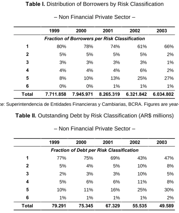
Table I. Distribution of Borrowers by Risk Classification
– Non Financial Private Sector –
1999 2000 2001 2002 2003
Fraction of Borrowers per Risk Classification
1 80% 78% 74% 61% 66% 2 5% 5% 5% 5% 2% 3 3% 3% 3% 3% 1% 4 4% 4% 4% 6% 2% 5 8% 10% 13% 25% 27% 6 0% 0% 1% 1% 1% Total 7.711.858 7.945.971 8.265.319 6.321.842 6.034.802
Source: Superintendencia de Entidades Financieras y Cambiarias, BCRA. Figures are year-end.
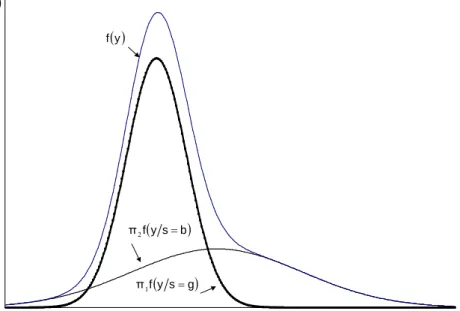
Table II. Outstanding Debt by Risk Classification (AR$ millions)
– Non Financial Private Sector –
1999 2000 2001 2002 2003
Fraction of Debt per Risk Classification
1 77% 75% 69% 43% 47% 2 5% 4% 5% 10% 8% 3 2% 3% 3% 10% 5% 4 5% 6% 6% 11% 8% 5 10% 11% 16% 25% 30% 6 1% 1% 1% 1% 2% Total 79.291 75.345 67.329 55.535 49.589
Source: Superintendencia de Entidades Financieras y Cambiarias, BCRA. Figures are year-end. After experiencing years of growth, the argentine economy entered a recession in 1999, which among other consequences affected banks’ loan portfolios with a reduction of the share of performing borrowers (i.e., borrowers classified 1 or 2). While on December 1999 performing borrowers and their corresponding obligations represented respectively 85% and 82% of the total, these shares where 79% and 74% in 2001. After three years of stagnation, though, the crisis unfolded in 2002, triggered by a deposit freeze, the devaluation of the argentine peso and the default of the public debt, dragging the economy into a more severe recession with
real GDP shrinking 11% that year. The crisis reinforced the worsening of banks’ loan portfolios, increasing the fraction of non-performing borrowers and debt, and reducing the depth of the financial system. Bank credit to the non-financial private sector fell from 23.3% of GDP in December 1999, to 19.2% in December 2001 and 7.5% in December 2003. Besides, by the end of 2003 nearly 50% of the outstanding bank credit to the non-financial private sector was in default.
III. Methodology
Following the approach employed in Carey (2000, 1998) we use a resampling-based Monte Carlo simulation to estimate conditional and unconditional distributions of the annual losses observed in banks’ loan portfolios, using the data contained in the public credit registry of the Central Bank of Argentina, Central de Deudores del
Sistema Financiero (CENDEU). The computations are performed controlling by type of obligor or portfolio (corporate, SME and retail) and by type of financial institution (bank and non-bank, public, foreign owned, cooperative, etc.). Therefore, for each year and each type of bank three conditional distributions are obtained, as well as one unconditional distribution for each combination of type of bank and portfolio. By this token, should differences exist in the credit policies followed by different types of institutions (i.e. private banks vs. public banks, banks vs. financial companies) these are likely to be captured by the shape of their respective distributions.
As explained in the introduction, the objective of the paper is to obtain conditional distributions for each of the five years comprised in the period 1999-2004: 1999-2000, 2000-2001, 2001-2002, 2002-2003 and 2003-2004. These estimates are deemed as conditional since, for sufficiently diversified or fine grained portfolios, their shape will generally depend on the realization of the systematic factor(s) and on
obligors’ asset or default correlation. In this paper, we assume that there is only one systematic factor affecting obligors’ credit stance, which is the state of the economy and is proxied by the observed behaviour of the GDP.
For each portfolio and type of bank an unconditional distribution is also computed. In this case, for each combination of portfolio and type of bank the behaviour of the borrowers in the period 1999-2004 is taken altogether in the simulation, therefore allowing for the coexistence of different patterns of credit risk in response to different realizations of the systematic factor.
Before estimating a conditional distribution a sub-set of the obligors’ population is assembled; this sub-set will later be used to perform the resampling. First, from the total population of obligors belonging to the non-financial private sector only those with a positive amount of outstanding debt at the outset of the chosen period are retained. Second, given that the conditional distribution is computed for one particular combination of type of bank and portfolio, we choose those borrowers that meet this criteria. Third, borrowers that are already in default at the outset of each period are removed from the sample. Besides, some obligors that exist at the outset of a period disappear from the CENDEU during the following 12 months. This is because they may either have defaulted, been written-off and removed from the bank’s balance sheet and from CENDEU, or they may have cancelled their debts and also been deleted from the CENDEU. In both cases they are removed from the sample as well; the empirical evidence found in Balzarotti, Gutiérrez Girault and Vallés (2006) shows that the potential bias introduced by removing these borrowers is negligible. For the remaining borrowers, their initial total indebtedness and eligible collateral with the bank are computed, and their risk classification in that bank one year ahead, be it indicative of default or not, is attached.
The sample constructed in this way enables the computation of an observed default rate and, together with assumptions regarding recovery rates, of a loss rate. The aforementioned procedure, while informative as to the loss experienced in the chosen portfolio, is a snapshot which yields no additional information such as what other values the loss rate may have taken and with what probability, what is the average loss rate or, perhaps more importantly, what are the worse loss rates that the portfolio may suffer, no matter how unlikely they are. Namely, we are interested in knowing the range of possible values that loan portfolios’ losses may take with their associated probability, which is the output of our resampling-based Monte Carlo simulation.
To perform the Monte Carlo simulation we construct many simulated portfolios by drawing borrowers randomly and with replacement from the corresponding sub-set for which the distribution is to be computed. When simulating the portfolios we tried to mimic as far as possible the actual characteristics of the segment under study. Therefore, besides limiting the data to those borrowers that met the characteristics of the portfolios to be modelled (type of borrower and of bank), the size of the simulated portfolios (measured by the number of obligors in them) was set to equal the average number of obligors in the portfolio under study, with a cap of 500 obligors for corporates and 1,000 for SMEs and retail. For example, when simulating the distribution of corporate clients of foreign banks, the simulated portfolios were constructed drawing randomly from a pool of corporate borrowers of foreign banks, with the restriction that the size of each portfolio matched the average size of this sort of portfolio, subject to the mentioned cap. In addition to this, the resampling introduces a source of randomness, and of error, in the results, which shrinks with the number of portfolios simulated. Our results didn’t show a clear
pattern of change when increasing the number of resamples from 5,000 to 20,000. Therefore, to ease the speed of computation but keeping the error as low as possible we limited the number of iterations to 10,000. Consequently, the results that follow in the paper were obtained resampling 10,000 portfolios according to the already explained data generation process. Having simulated 10,000 portfolios of the desired group of borrowers, the loss rate is estimated for each portfolio. The resulting set of 10,000 loss rates, which can be displayed diagrammatically in a histogram, constitutes our estimated loan loss distribution.
To illustrate the procedure with an example, assume we want to understand the behaviour of the loss rate of loans granted by foreign banks to corporate borrowers in a specific period, such as December 2002 – December 2003. After removing the borrowers already in default in December 2002, as well as those that disappeared during the course of the year, we attach to the remaining ones their risk classification in December 2003. Subsequently we simulate 10,000 portfolios drawing randomly from the sub-set of borrowers with the restriction that the number of obligors is consistent with the observed size of the portfolio being analysed, and for each simulated portfolio we compute the loss rate. Finally, with the 10,000 loss rates we compute the average (expected) loss and different percentiles that will provide us with measures of unexpected losses, at various confidence levels.
Conditional distributions summarize the potential credit losses that banks may experience as a result of credit events in one particular year and thus, for one particular realization of the systematic factor (the behaviour of the GDP). Conditioning in the realization of the systematic factor, the variability of the portfolio losses displayed in the distribution results from the randomness introduced by the resampling procedure coupled with the observed default rate in the assembled
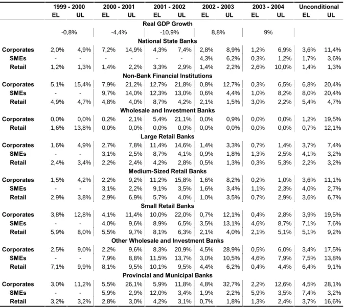
sub-set, the heterogeneity of the loans in the portfolio and the existence of collaterals. However, when comparing observed loss rates in different periods of time, their difference may result not only from the abovementioned factors but also from the state of the economy. The unconditional distribution may also be understood as being a weighted average of the distributions observed in different realizations of the systematic factor, as a result of which the dynamic of the borrowers switches from one of low risk to a dynamic of high risk. Thus, the unconditional distribution is the mixture of conditional distributions that switch between regimes of high or low risk according to the observed realizations of the systematic factor. Figure I shows an example of the interpretation of unconditional distributions as the summation of densities corresponding to different regimes, weighted by the likelihood of occurrence of each regime3.
Figure I. Unconditional distributions as mixture-distributions
In Figure I f(y/s=b) represents the distribution of yt/st=b, which is assumed to
be normal with mean 2 and variance 8, and that may represent the behaviour of losses in bad realizations of the systematic factor (s=b) (i.e., yt/st = b ~ N(2,8)). On
y y s g f ð1 ys b f ð2 y f y f
the other hand, representing the behaviour of losses in good realizations of the systematic factor the graph shows yt/st = g ~ N(0,1). The unconditional distribution is
obtained as the vertical summation of densities for each level of loss, weighted by the probability of occurrence of each state of the economy. The difference between the two conditional densities is reflecting that during economic downturns credit losses are higher on average and more volatile.
IV. Empirical Results
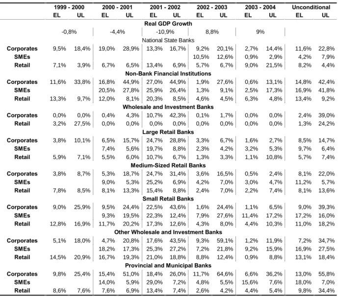
The principal results of the simulations are summarized in tables III and IV. In Table III we assume that in each defaulted loan the loss equals 50% of the uncovered tranche of the exposure. Results in Table IV reflect a much conservative stance and assume the loss amounts to 100% of the uncovered tranche plus 50% of the collateral. Therefore the difference in the expected and unexpected losses for the same portfolio (i.e., type of borrower and of bank) in both tables is the assumption regarding the recoveries or the effective Loss Given Default (LGD), since in both cases the underlying loss rate is the same. In what follows, the discussion will be centred on the results displayed in the first table. Nevertheless, and taking into consideration that during economic downturns LGDs are likely to be larger than in normal times, since the market value of collaterals may decline, the results shown in Table IV are more suitable to assess the behaviour of credit losses during deep recessions, such as the 2001-2002 period.
Table III shows, for each type of bank and borrower, the resampled conditional expected and unexpected losses. In each case the simulations were computed for each of the abovementioned 12-month periods, while on the other hand the unconditional estimates correspond to the whole 1999-2004 period. Unexpected
losses are those that exceed the expected ones, and that usually correspond to the 90th, 95th, 99th and 99.9th percentiles. The latter, however, are of particular relevance since most model-based portfolio models yield estimates of the unexpected loss at this confidence level, such as Basel II’s IRB. Therefore, to facilitate the comparability of results with the model-based alternatives only the unexpected losses at the 99.9% confidence are shown.
Table III. Expected and Unexpected Losses (99.9% confidence level) - Scenario I: loss equals 50% of uncovered exposure -
1999 - 2000 2000 - 2001 2001 - 2002 2002 - 2003 2003 - 2004 Unconditional
EL UL EL UL EL UL EL UL EL UL EL UL
Real GDP Growth
-0,8% -4,4% -10,9% 8,8% 9%
National State Banks
Corporates 2,0% 4,9% 7,2% 14,9% 4,3% 7,4% 2,8% 8,9% 1,2% 6,9% 3,6% 11,4%
SMEs - - - 4,3% 6,2% 0,3% 1,2% 1,7% 3,6%
Retail 1,2% 1,3% 1,4% 2,2% 3,3% 2,9% 1,4% 2,2% 2,6% 10,0% 1,4% 1,3%
Non-Bank Financial Institutions
Corporates 5,1% 15,4% 7,9% 21,2% 12,7% 21,8% 0,8% 12,7% 0,3% 6,5% 6,8% 20,4%
SMEs - - 9,7% 14,0% 12,3% 13,0% 0,6% 4,4% 1,0% 8,2% 8,0% 20,4%
Retail 4,9% 4,7% 4,8% 4,0% 8,7% 4,2% 2,1% 1,5% 3,0% 2,2% 5,4% 4,7%
Wholesale and Investment Banks
Corporates 0,0% 0,0% 0,2% 2,1% 5,4% 21,1% 0,0% 0,9% 0,0% 0,0% 1,2% 19,5%
Retail 1,6% 13,8% 0,0% 0,0% 0,0% 0,0% 0,0% 0,0% 0,0% 0,0% 0,7% 12,1%
Large Retail Banks
Corporates 1,6% 4,9% 2,7% 7,8% 11,4% 14,6% 1,4% 3,3% 0,7% 1,4% 3,7% 7,4%
SMEs - - 3,1% 2,5% 8,7% 4,1% 0,9% 1,8% 1,3% 2,5% 4,1% 3,2%
Retail 2,4% 3,4% 2,2% 2,4% 4,2% 2,8% 0,5% 1,3% 0,3% 5,3% 2,2% 3,2%
Medium-Sized Retail Banks
Corporates 1,5% 4,2% 2,2% 9,2% 11,2% 15,8% 1,6% 8,2% 0,2% 1,0% 3,6% 11,1%
SMEs - - 3,1% 2,2% 9,1% 3,5% 1,6% 3,4% 1,1% 2,3% 4,0% 2,7%
Retail 2,9% 3,8% 2,9% 6,9% 5,7% 4,0% 1,0% 3,5% 0,7% 2,9% 3,6% 6,7%
Small Retail Banks
Corporates 3,8% 12,8% 4,1% 11,4% 10,0% 22,0% 0,7% 12,1% 0,4% 2,8% 3,9% 19,5%
SMEs - - 4,0% 9,6% 8,9% 6,5% 3,5% 13,1% 4,6% 8,7% 7,1% 7,6%
Retail 5,9% 8,0% 5,5% 9,7% 8,1% 6,3% 2,1% 4,0% 2,1% 5,1% 5,1% 9,2%
Other Wholesale and Investment Banks
Corporates 2,5% 9,0% 2,2% 9,6% 8,3% 20,9% 4,5% 28,9% 0,5% 6,0% 3,4% 17,5%
SMEs - - 7,9% 8,8% 11,5% 13,7% 3,0% 10,5% 4,6% 7,9% 7,5% 13,8%
Retail 7,1% 9,9% 8,1% 9,5% 10,1% 9,5% 4,4% 6,2% 0,4% 4,4% 6,4% 9,1%
Provincial and Municipal Banks
Corporates 3,0% 11,2% 5,5% 26,1% 5,9% 11,8% 4,8% 32,7% 2,2% 12,6% 4,5% 28,1%
SMEs - - 5,9% 2,9% 12,0% 3,4% 1,9% 2,2% 5,9% 3,5% 7,4% 3,2%
Table IV. Expected and Unexpected Losses (99.9% confidence level) - Scenario II: loss equals uncovered exposure plus 50% of collateral -
1999 - 2000 2000 - 2001 2001 - 2002 2002 - 2003 2003 - 2004 Unconditional
EL UL EL UL EL UL EL UL EL UL EL UL
Real GDP Growth
-0,8% -4,4% -10,9% 8,8% 9%
National State Banks
Corporates 9,5% 18,4% 19,0% 28,9% 13,3% 16,7% 9,2% 20,1% 2,7% 14,4% 11,6% 22,8%
SMEs 10,5% 12,6% 0,9% 2,9% 4,2% 7,9%
Retail 7,1% 3,9% 6,7% 6,5% 13,4% 6,9% 5,7% 6,7% 9,0% 21,5% 8,2% 4,4%
Non-Bank Financial Institutions
Corporates 11,6% 33,8% 16,8% 44,9% 27,0% 44,9% 1,9% 27,6% 0,6% 13,1% 14,8% 42,4%
SMEs 20,5% 27,8% 25,9% 26,4% 1,3% 9,1% 2,5% 17,3% 16,9% 41,8%
Retail 13,3% 9,7% 12,0% 8,1% 20,3% 8,5% 4,6% 4,5% 6,3% 4,8% 13,4% 9,2%
Wholesale and Investment Banks
Corporates 0,0% 0,0% 0,4% 4,3% 10,7% 42,3% 0,1% 1,7% 0,0% 0,0% 2,4% 39,0%
Retail 3,2% 27,5% 0,0% 0,0% 0,0% 0,0% 0,0% 0,0% 0,0% 0,0% 1,3% 24,2%
Large Retail Banks
Corporates 3,8% 10,1% 6,5% 15,7% 24,7% 28,8% 3,3% 6,7% 1,6% 2,7% 8,5% 14,7%
SMEs 7,4% 5,6% 19,7% 8,8% 2,3% 4,2% 3,2% 5,3% 9,7% 6,4%
Retail 5,9% 7,1% 5,5% 6,0% 10,7% 6,7% 1,3% 3,3% 1,1% 10,8% 5,7% 7,4%
Medium-Sized Retail Banks
Corporates 3,8% 8,7% 5,3% 18,7% 24,7% 31,4% 3,6% 16,5% 0,5% 2,4% 8,1% 22,0%
SMEs 9,0% 5,3% 25,2% 6,9% 4,2% 7,0% 3,0% 4,7% 11,2% 5,7%
Retail 7,8% 8,5% 8,1% 13,3% 15,4% 8,8% 2,4% 7,0% 2,2% 7,4% 8,1% 13,6%
Small Retail Banks
Corporates 9,0% 25,9% 9,5% 24,4% 22,5% 43,6% 1,6% 24,4% 1,1% 6,5% 9,0% 39,3%
SMEs 9,3% 19,5% 22,3% 12,4% 7,9% 27,6% 11,4% 17,2% 17,2% 16,0%
Retail 12,8% 16,9% 11,7% 20,2% 17,3% 12,6% 4,3% 8,0% 4,4% 10,3% 11,0% 18,2%
Other Wholesale and Investment Banks
Corporates 5,1% 18,0% 4,7% 20,8% 17,6% 43,5% 9,3% 59,1% 1,2% 11,9% 7,2% 34,7%
SMEs 18,2% 17,3% 25,3% 27,2% 7,2% 21,8% 9,2% 15,9% 16,9% 27,5%
Retail 14,5% 20,9% 16,7% 19,3% 21,0% 18,8% 8,8% 12,4% 0,9% 8,8% 13,1% 18,4%
Provincial and Municipal Banks
Corporates 9,8% 25,4% 15,4% 51,0% 18,4% 26,0% 11,7% 64,6% 6,6% 36,2% 13,0% 55,8%
SMEs 14,0% 5,9% 29,0% 7,2% 4,8% 5,5% 15,6% 7,6% 18,0% 7,0%
Retail 8,6% 7,6% 7,6% 6,9% 13,4% 7,4% 2,6% 4,2% 4,4% 5,4% 9,8% 34,4%
Conditional Distributions
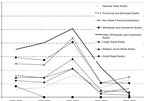
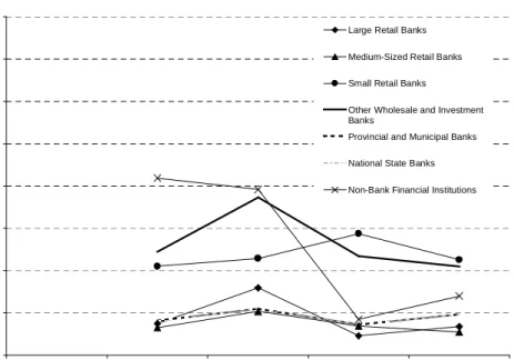
The results of the simulated conditional distributions show that, across the economic cycle, the expected losses corresponding to the different portfolios are quite correlated, although their behaviour presents differences. Figures II, III and IV show the conditional expected losses for corporates, SMEs and the retail portfolio, by type of financial institution. As expected, conditional expected losses are cyclical: around 2% in years of high economic growth (such as 2003 and 2004), increasing in 2001 up to 8% in the case of the retail portfolio and corporates and 10% for SMEs. It
is worth mentioning that by December 2001 the argentine economy had been in recession for three years, with real GDP falling 3.4% in 1999, 0.8% in 2000 and 4.4% in 2001. At the outset of the year 2002, the devaluation of the argentine Peso and the default of the public debt transformed the recession into a major crisis, with real GDP falling 11% that year. As a result of this, the expected loss rates conditional on the events of 2002 soared to 12% in the case of corporates and SMEs, and to 10% for the retail portfolio.
Figure II. Conditional Expected Losses: Retail Portfolio
Figure III. Conditional Expected Losses: SME Portfolio
2% 4% 6% 8% 10% 12% 14%
National State Banks
Provincial and Municipal Banks
Non-Bank Financial Institutions
Other Wholesale and Investment Banks
Large Retail Banks
Medium-Sized Retail Banks
Small Retail Banks 0% 2% 4% 6% 8% 10% 12% 14% 1999-2000 2000-2001 2001-2002 2002-2003 2003-2004 National State Banks
Provincial and Municipal Banks
Non-Bank Financial Institutions
Wholesale and Investment Banks
Other Wholesale and Investment Banks
Large Retail Banks
Medium-Sized Retail Banks
Figure IV. Conditional Expected Losses: Corporate Portfolio
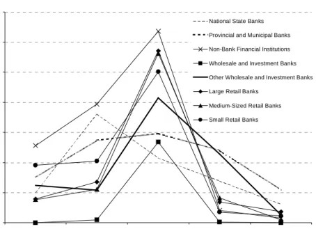
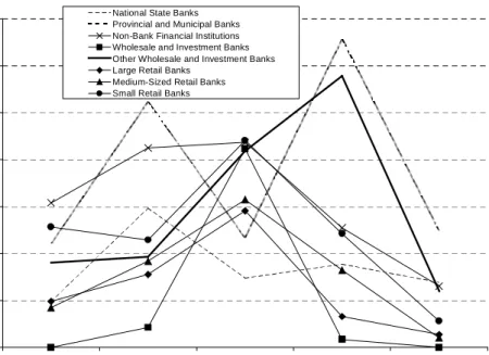
Figures II - IV above also show that the cyclical pattern of expected losses for each type of borrower is very similar across all the institutions, but it shows differences between types of borrowers. On the other hand, figures V, VI and VII below depict the behaviour of the conditional unexpected losses. In the case of the retail and SME portfolio, our results show that although the estimates react to the business cycle, they are less sensible to the state of the economy than the expected losses. With the exception of wholesale and investment banks, unexpected losses of the retail portfolio range between 0% and 10% during the three years comprised between 1999 and 2002, peaking slightly during 2001, and reduced subsequently to a range below 5% in years of high economic growth. The unexpected losses of SMEs present a similar pattern, although they take values up to 15% (on top of the expected losses) and the effect of the state of the economy on them seems to be even milder. Finally, corporate borrowers are much more responsive to the realizations of the systematic factor. With the exception of state-owned banks, the unexpected losses of this portfolio increased significantly during 2002 in response to the economic crisis, with unexpected losses in some cases above 20% of the
0% 2% 4% 6% 8% 10% 12% 14% 1999-2000 2000-2001 2001-2002 2002-2003 2003-2004 National State Banks
Provincial and Municipal Banks
Non-Bank Financial Institutions
Wholesale and Investment Banks
Other Wholesale and Investment Banks
Large Retail Banks
Medium-Sized Retail Banks
portfolio and on top of the expected losses. These findings regarding the higher sensitivity of corporate obligors to the realizations of the systematic factor and, conversely, the fact that defaults of retail and SME obligors are more idiosyncratic and less dependent on the economic cycle, are reflected in the calibration of the IRB approach, as explained in BCBS (2004).
Figure V. Conditional Unexpected Losses: Retail Portfolio
Figure VI. Conditional Unexpected Losses: SME Portfolio
0% 5% 10% 15% 20% 25% 30% 35% 1999-2000 2000-2001 2001-2002 2002-2003 2003-2004 National State Banks
Provincial and Municipal Banks Non-Bank Financial Institutions Wholesale and Investment Banks
Other Wholesale and Investment Banks Large Retail Banks
Medium-Sized Retail Banks
Small Retail Banks
0% 5% 10% 15% 20% 25% 30% 35% 2000-2001 2001-2002 2002-2003 2003-2004 National State Banks
Provincial and Municipal Banks
Non-Bank Financial Institutions
Other Wholesale and Investment Banks
Large Retail Banks
Medium-Sized Retail Banks
Figure VII. Conditional Unexpected Losses: Corporate Portfolio
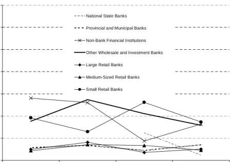
The findings regarding the conditional expected and unexpected losses shown thus far reflect the shifting of the loss distributions as a consequence of the realizations of the systematic factor. Those findings, also, reflect the higher loss volatility observed in bad years (recessions), and the lower volatility observed in good years (expansions of the economy). Figures VIII, IX and X show the impact of the systematic factor on (conditional) loss volatilities.
Figure VIII. Conditional Loss Volatilities: Retail Portfolio
0% 1% 2% 3% 4% 5% 6% 7% 8% 1999-2000 2000-2001 2001-2002 2002-2003 2003-2004 Wholesale and Investment Banks
Large Retail Banks
Medium-Sized Retail Banks
Small Retail Banks
Other Wholesale and Investment Banks
Provincial and Municipal Banks
National State Banks
Non-Bank Financial Institutions 0% 5% 10% 15% 20% 25% 30% 35% 1999-2000 2000-2001 2001-2002 2002-2003 2003-2004 National State Banks
Provincial and Municipal Banks Non-Bank Financial Institutions Wholesale and Investment Banks Other Wholesale and Investment Banks Large Retail Banks
Medium-Sized Retail Banks Small Retail Banks
Figure IX. Conditional Loss Volatilities: SME Portfolio
Figure X. Conditional Loss Volatilities: Corporate Portfolio
0% 1% 2% 3% 4% 5% 6% 7% 8% 1999-2000 2000-2001 2001-2002 2002-2003 2003-2004 Wholesale and Investment Banks
Large Retail Banks Medium-Sized Retail Banks Small Retail Banks
Other Wholesale and Investment Banks Provincial and Municipal Banks National State Banks Non-Bank Financial Institutions
While the three figures reflect the behaviour of unexpected losses through-the-cycle, in all three cases our simulated loss volatilities show the expected behaviour, in the sense that in years of bad realizations of the systematic factor the loss volatility is higher, and lower in good years.
0% 1% 2% 3% 4% 5% 6% 7% 8% 1999-2000 2000-2001 2001-2002 2002-2003 2003-2004 Large Retail Banks
Medium-Sized Retail Banks
Small Retail Banks
Other Wholesale and Investment Banks
Provincial and Municipal Banks
National State Banks
Unconditional Distributions
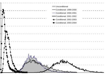
In this sub-section we discuss the results obtained when computing the unconditional distributions, applying the resampling-based simulation to a chosen sub-set of borrowers but for the period 1999-2004 altogether. The resulting distribution can be understood as an average of the conditional distributions that correspond to different realizations of the systematic factor, weighted by the likelihood of occurrence of that particular realization.
Figure XI shows an example of the unconditional distribution of retail obligors of big retail banks. In the graph it can be seen how the conditional distributions shift according to the realizations of the systematic factor, with bad realizations shifting the conditional distributions to the right, increasing their mean (expected loss) and standard deviation. In the figure below the unconditional distribution is indicated with a grey area.
Figure XI. Unconditional Distribution as Mixture of Conditional Distributions: Retail Portfolio of Big Retail Banks
0% 1% 2% 3% 4% 5% 6% 7% 8% 9% 0 ,0 % 0 ,3 % 0 ,5 % 0 ,7 % 0 ,9 % 1 ,2 % 1 ,4 % 1 ,6 % 1 ,8 % 2 ,1 % 2 ,3 % 2 ,5 % 2 ,7 % 3 ,0 % 3 ,2 % 3 ,4 % 3 ,6 % 3 ,9 % 4 ,1 % 4 ,3 % 4 ,5 % 4 ,8 % 5 ,0 % 5 ,2 % 5 ,4 % 5 ,7 % 5 ,9 % 6 ,1 % 6 ,3 % 6 ,6 % Unconditional Conditional: 1999-2000 Conditional: 2000-2001 Conditional: 2001-2002 Conditional: 2002-2003 Conditional: 2003-2004
The resulting estimations of unconditional expected and unexpected losses (at the 99.9% confidence level in the last case) are shown by type of borrower and bank in figures XII through XIV.
Figure XII. Expected and Unexpected Unconditional Losses: Retail Portfolio
Figure XIII. Expected and Unexpected Unconditional Losses: SME Portfolio
1,4% 3,7% 5,4% 0,7% 6,4% 2,2% 3,6% 5,1% 1,3% 16,6% 4,7% 12,1% 9,1% 3,2% 6,7% 9,2% 0% 5% 10% 15% 20% 25% 30% 35% National State Banks Provincial and Municipal Banks Non-Bank Financial Institutions Wholesale and Investment Banks Other Wholesale and Investment Banks Large Retail Banks Medium-Sized Retail Banks Small Retail Banks EL UL 1,7% 7,4% 8,0% 7,5% 4,1% 4,0% 7,1% 3,6% 3,2% 20,4% 13,8% 3,2% 2,7% 7,6% 0% 5% 10% 15% 20% 25% 30% 35% National State Banks Provincial and Municipal Banks Non-Bank Financial Institutions Other Wholesale and Investment Banks Large Retail Banks Medium-Sized Retail Banks Small Retail Banks EL UL
Figure XIV. Expected and Unexpected Unconditional Losses: Corporate Portfolio
The results reflect our findings regarding the behaviour of corporate obligors’ losses through-the-cycle: their unconditional unexpected losses are particularly larger than those of SMEs and retail obligors, therefore meriting larger capital requirements as reflected in the design of the IRB approach. Notwithstanding the type of borrower involved, there are also clear differences in unconditional distributions across banks, with large and medium-sized retail banks and national state banks showing the lowest risk, measured by the loss rate at the 99.9% confidence level (i.e., the 99.9th percentile of the unconditional loss distribution). Within each asset class, banks’ risk profile varies considerably by type of bank. In the case of the retail portfolio, provincial and municipal banks have the largest loss at the 99.9th percentile, 20% of its retail portfolio, followed by wholesale and investment banks. Regarding SMEs, non-bank financial institutions are those with the riskiest portfolio, with a loss rate at the 99.9th percentile of more than 28% of the portfolio. On the other hand, national state banks and large retail banks have the lowest loss rates at that percentile of the
3,6% 4,5% 6,8% 1,2% 3,4% 3,7% 3,6% 3,9% 11,4% 28,1% 20,4% 19,5% 17,5% 7,4% 11,1% 19,5% 0% 5% 10% 15% 20% 25% 30% 35% National State Banks Provincial and Municipal Banks Non-Bank Financial Institutions Wholesale and Investment Banks Other Wholesale and Investment Banks Large Retail Banks Medium-Sized Retail Banks Small Retail Banks EL UL
tail distribution. As to the corporates, provincial and municipal banks have loss rates higher than 30% at a 99.9% Value-at-Risk, followed by the non-bank financial institutions and small retail banks. In general, the abovementioned differences in risk profiles may be attributed to differences in the granularity of the corresponding portfolios, in the respective obligors sensitivity to the systematic factor and in their risk management policies and tools (i.e., application and behavioural scorings). In this last case, it is worth mentioning that among the financial institutions with the highest risk profiles are some which may not seem proficient enough or with the necessary expertise with respect to the corresponding borrowers, such as wholesale and investment banks in the retail portfolio, non-bank financial institutions with SMEs and corporates and small retail banks with corporates.
Comparison with a model-based approach: the advanced IRB
Among other possible uses, the results obtained with this methodology can be compared with Basel II’s IRB approach. In what follows, we perform an exercise adapted from Majnoni, Miller and Powell (2004) in which we compare the capital requirements needed to cover unexpected losses at the 99.9% confidence level of our unconditional distributions, with those resulting from the IRB approach. Taking the estimated unconditional expected loss of any portfolio, assuming its corresponding default rate is a good proxy of the average PD of the obligors and that the exposure at default equals their outstanding debt, we find an implicit LGD. To perform this computations we use unconditional estimates since they incorporate the loss experience in adverse scenarios. With these risk dimensions we compute the (advanced) IRB capital requirements. The results, expressed as the ratio of the IRB
capital requirements to the Monte Carlo estimated capital requirements, are shown in Table V.
Table V. IRB capital requirements vs. Non-parametric Monte Carlo based
Corporates SMEs Retail
National State Banks 0.8 3.4 2.5
Non-Bank Financial Institutions 0.9 0.9 1.8
Wholesale and Investment Banks 0.6 - 0.9
Large Retail Banks 1.8 3.6 1.6
Medium-Sized Retail Banks 1.0 4.1 1.2
Small Retail Banks 0.6 2.0 1.2
Provincial and Municipal Banks 0.5 5.0 0.5
The results show that, on average, the IRB yields capital requirements which would be insufficient to cover unexpected losses at the 99.9% confidence level for corporate obligors. This effect is particularly important for wholesale and investment, small retail and provincial and municipal banks. Besides suggesting a possible miscalibration of the IRB model, these results may reflect the fact that these banks’ portfolios are not sufficiently fine-grained. Conversely, for the retail and SME portfolios we find that the coverage produced by and IRB approach would be overly conservative, yielding capital requirements more than enough to cover unexpected losses at the 99.9% VaR. For example, in the case of large retail banks IRB capital requirements for SME obligors would be 260% larger than the unexpected losses, and 60% larger in the case of retail borrowers. Our results for corporates reinforce those obtained in Majnoni, Miller and Powell (2004) who also found that the IRB approach yielded insufficient coverage for corporate obligors. However, their resampled distributions included corporate and some SME obligors, did not control by type of bank (was performed for the whole financial system as a whole) and corresponded to the period 2000-2001 only.
V. Conclusions
In this paper we used data of the public credit registry of the Central Bank of Argentina to implement a non-parametric method to estimate loan portfolio loss distributions. The method, which is a resampling-based Monte Carlo simulation, enabled us to obtain conditional distributions for the five 12-month periods comprised between 1999 and 2004, and an unconditional distribution for the whole period. In both cases, separate computations where performed by type of borrower and bank. In all cases the estimated distributions allow the computation of economic (risk-based) measures of expected and unexpected losses for credit risk, to be covered with provisions and capital requirements. However, whether the supervisor must use conditional or unconditional measures to set the prudential regulation depends, among other factors, on the degree of risk sensitivity the regulation is expected or desired to show, and on the national supervisor’s leeway to deal with the prociclicality that conditional measures exacerbate.
As it was explained during the paper, unconditional distributions can be interpreted as an average of the conditional distributions. Therefore, had the exercise in this paper included information of the years 2005 and 2006, in which the economy grew at 9.2% and 8.5% and with obligors’ average default rates at 3.2% and 3.6% respectively, the estimated unconditional expected and unexpected losses would have been lower than those here obtained (shown in tables III and IV). According to the information of the BCRA, while at the end of 2003 only 66% of the obligors of the financial system were risk classified as 1 (see Table I), by the end of 2006 that fraction had risen to 86%. Therefore, for this methodology to be useful in bank regulation and supervision it is of paramount importance that the model is computed
with a sample that covers a sufficiently long time period, and that its estimates are updated on a regular basis.
The comparison between our resampled unconditional unexpected losses and the IRB capital requirements for the same portfolios allows to detect discrepancies between risk and coverage. These may be caused by less than sufficient granularity in banks’ portfolios or by problems in the calibration of the IRB. Our study shows there is a tendency of IRB capital requirements to exceed unexpected losses for SMEs and the retail portfolio, while they fall short in the case of corporate obligors. In this case, our findings support similar results obtained for corporate obligors of argentine banks in Majnoni, Miller and Powell (2004).
References
Balzarotti, V., M. A. Gutiérrez Girault y V. A. Vallés (2006). “Modelos de Scoring Crediticio con Muestras Truncadas y su Validación”, Banco Central de la República Argentina.
Basel Committee on Banking Supervision (2004). “An Explanatory Note on the Basel II IRB Risk Weight Functions”, Bank for International Settlements.
Carey, M. (1998). “Credit Risk in Private Debt Portfolios”, The Journal of Finance, Vol. LIII, N° 4, pp.1363-1387.
Carey, M. (2000). “Dimensions of Credit Risk and their Relationship to Economic Capital Requirements”, National Bureau of Economic Research, WP 7629.
CreditMetrics (1997). “Technical Document”, J.P. Morgan.
Credit Suisse Financial Products (1997). “CreditRisk+: A Credit Risk Management Framework”, Credit Suisse First Boston.
Efron, B. (1979). “Bootstrap Methods: Another Look at the Jacknife”, The Annals of Statistics, Vol. 7, N° 1, pp. 1-26.
Gordy, M. (2002). “A Risk-Factor Model Foundation for Ratings-Based Bank Capital Rules”, Board of Governors of the Federal Reserve System.
Hamilton, J. D. (1994). Time Series Analysis, Princeton University Press, Princeton, New Jersey
Majnoni, G., M. Miller and A. Powell (2004). “Bank Capital and Loan Loss Reserves under Basel II: Implications for Latin America and Caribbean Countries”, The World Bank and Universidad Torcuato Di Tella.
Vasicek, O. A. (1984). “Credit Valuation”, K.M.V.
Wilson, T. (1997). “Portfolio Credit Risk”, Risk Magazine, pp. 111–117. Wilson, T. (1997). “Portfolio Credit Risk”, Risk Magazine, pp. 56–61.