An Optimized Linear Model Predictive Control Solver
for Online Walking Motion Generation
Dimitar Dimitrov, Pierre-Brice Wieber, Olivier Stasse, Hans Joachim Ferreau, Holger Diedam
Abstract— This article addresses the fast solution of a Quadratic Program underlying a Linear Model Predictive Control scheme that generates walking motions. We introduce an algorithm which is tailored to the particular requirements of this problem, and therefore able to solve it efficiently. Different aspects of the algorithm are examined, its computational complexity is presented, and a numerical comparison with an existing state of the art solver is made. The approach presented here, extends to other general problems in a straightforward way.
I. INTRODUCTION
The difficulty in generating stable walking motions is mostly due to the fact that moving one’s Center of Mass (CoM) entirely relies on the unilateral contact forces between the feet and the ground [1]. In the presence of disturbances, this restriction severely limits the capacity of the system to follow predefined motions. It is necessary therefore to generate walking motions which are always adapted online to the current state of the system.
This issue is addressed in [2] through a Zero Moment Point (ZMP) Preview Control scheme that generates dynam-ically stable motions for a humanoid robot by approximating its nonlinear dynamics with the linear dynamics of a point mass. The walking motion generation problem is formulated then as a typical infinite horizon Linear Quadratic Regulator (LQR). This approach explicitly accounts for the system state and leads to fast computations.
One disadvantage of this scheme is that it does not explicitly account for the constraints on the ZMP, which must always lie in the support polygon: in case of disturbances, the system’s response can overshoot the boundaries of this polygon. This limitation is addressed in [3], where instead of solving an infinite horizon LQR, the utilization of a receding horizon LQR with constraints is proposed, in other words, a Linear Model Predictive Control scheme (LMPC). In [4] the authors develop the idea further by using an augmented state vector that addresses the problem of feet repositioning in the presence of strong disturbances.
The guarantee given by this LMPC scheme of keeping the system’s response within a given set of constraints comes at a price of increased computation demands. At each control Dimitar Dimitrov is with Orebro¨ University - Sweden,
Pierre-Brice Wieber is with INRIA Grenoble - France,
Olivier Stasse is with JRL - Japan,[email protected]
Hans Joachim Ferreau is with KU Leuven - Belgium,
Holger Diedam is with Heidelberg University - Germany,
step, the application of this LMPC scheme amounts to forming and solving a Quadratic Program (QP) [5].
A more efficient formulation of this LMPC scheme was proposed in [6]. The authors proposed the utilization of a variable sampling time scheme, in combination with a method for developing a reliable guess for the active con-straints at the solution by introducing the notion of “sliding constraints”. It is shown that such a guess can drastically reduce the computational burden for each iteration.
In practice, the solution of the underlying QP is left to state of the art QP solvers [7]. Even though such solvers implement very efficient algorithms, in most cases they do not make use of the properties of each particular problem, which could sometimes speed up computations a lot.
In this article, we introduce an optimized algorithm for the fast solution of a particular QP in the context of LMPC for online walking motion generation. It can be classified as aprimal active set method with range space linear algebra. We motivate our choice by analyzing the requirements of our problem. Different aspects of the algorithm are examined, and its computational complexity is presented. We compare then the run-time of our algorithm with a state of the art solver.
The article is organized as follows: in Section II we briefly outline the LMPC scheme presented in [3]. In Section III we discuss alternative methods for the solution of a QP, and analyze how do their properties reflect on our problem. In Section IV we present our algorithm and discuss its features, state its complexity and compare it with the algorithm in [8]. Finally, in Section V we present a numerical comparison with QL [7].
II. ANLMPCSCHEME GENERATING WALKING MOTIONS The Model Predictive Control (MPC) scheme introduced in [2], [3] for generating walking motions works primarily with the motion of the CoM of the walking robot. In order to obtain an LMPC scheme, it is assumed that the robot walks on a constant horizontal plane, and that the motion of its CoM is also constrained to a horizontal plane at a distance h above the ground, so that its position in space can be defined using only two variables(x, y).
Only trajectories of the CoM with piecewise constant jerks...x and ...y over time intervals of constant length T are considered. That way, focusing on the state of the system at the instantstk=kT, ˆ xk= x(tk) ˙ x(tk) ¨ x(tk) , yˆk= y(tk) ˙ y(tk) ¨ y(tk) , (1)
2009 IEEE International Conference on Robotics and Automation Kobe International Conference Center
the integration of the constant jerks over the time intervals of lengthT gives rise to a simple recursive relationship:
ˆ xk+1=Axˆk+B ... x(tk), (2) ˆ yk+1=Ayˆk+B ... y(tk), (3)
with a constant matrixAand vector B. Then, the position (zx, zy)
of the ZMP on the ground corresponding to the motion of the CoM of the robot is approximated by considering only a point mass fixed at the position of the CoM instead of the whole articulated robot:
zxk = 1 0 −h/g ˆ xk, (4) zyk = 1 0 −h/g ˆ yk, (5)
withhthe constant height of the CoM above the ground and g the norm of the gravity force.
Using the dynamics (2) recursively, we can derive a relationship between the jerk of the CoM and the position of the ZMP over time intervals of lengthN T:
Zkx+1=Pzsxˆk+Pzu ... Xk, (6) Zky+1=Pzsyˆk+Pzu ... Yk, (7)
with constant matricesPzs∈R
N×3 andP zu∈R N×N , with Zkx+1= zx k+1 .. . zx k+N , ... Xk = ... xk .. . ... xk+N−1 , (8)
and similar definitions for Zky+1 and ... Yk.
In order for a motion of the CoM to be feasible, we need to ensure that the corresponding position of the ZMP always stays within the convex hull of the contact points of the feet of the robot on the ground [1]. This constraint can be expressed at the instantstkfor a whole time interval of length
N T as: blk+1≤Dk+1 Zx k+1 Zky+1 ≤buk+1, (9) with a Dk+1 ∈ Rm×2N a matrix varying with time but extremely sparse and well structured, with only2mnon zero values on 2 diagonals.
The LMPC scheme involves then a quadratic cost which is minimized in order to generate a “stable” motion [3], [6], leading to a canonical Quadratic Program (QP)
min u 1 2u TQu+pT ku (10) with u= ... X...k Yk , (11) Q= Q′ 0 0 Q′ (12) where Q′
is a positive definite constant matrix, and pTk = ˆxTk yˆ T k Psu 0 0 Psu (13) wherePsuis also a constant matrix (see [4] for more details).
With the help of the relationships (6) and (7), the con-straints (9) on the position of the ZMP can also be repre-sented as constraints on the jerkuof the CoM:
b′l k+1≤Dk+1 Pzu 0 0 Pzu u≤b′u k+1. (14) Since the matrixQis positive definite and the set of linear constraints (14) forms a (polyhedral) convex set, there exists a unique global minimizeru∗
[9].
The number of variables in the minimization problem (10) is equal ton= 2N and the number of constraints (14) is of the same order,m≈2N. Typical uses of this LMPC scheme considerN= 75andT = 20ms, for computations made on
a time intervalN T = 1.5s, approximately the time required to make 2 walking steps [6]. This leads to a QP which is typically considered as small or medium sized.
Another important measure to take into account about this QP is the number ma of active constraints at the
minimumu∗
, the number of inequalities in (14) which hold as equalities. We have observed that at steady state, this number is usually very low, ma ≤m/10, and even in the
case of strong disturbances, we can observe that it remains low, with usuallyma ≤m/2 [6].
III. GENERAL DESIGN CHOICES FOR AQPSOLVER
A. Interior point or active set method
The choice of an algorithm that can solve efficiently a QP with the above characteristics is not unique. Fast and reliable solvers based oninterior pointoractive setmethods are generally available and there has been a great deal of research related to the application of both approaches in the context of MPC [5], [10], [11], [12].
Finding the solution of a QP in the case when the set of active constraints atu∗
is known, amounts to solving a linear system of equations that has a unique solution [9]. Active set methods are iterative processes that exploit the above property and try to guess at each iteration which are the active constraints at the minimumu∗
. They usually consider active constraints one at a time, inducing a computation time directly related to the number of active constraints. On the contrary, the computation time of interior point methods is relatively constant, regardless of the number of active constraints. However, this constant computation time can be large enough to compare unfavorably with active set methods in cases such as the one here, a small QP with relatively few active constraints.
The question of “warm-starting” the solvers is the final important feature to consider. Indeed, what we have to solve is not a unique QP but a series of QPs at each time tk which appear to be sequentially related. It is possible
then to use information about the solution computed at time tk to accelerate the computation of the solution at
timetk+1 [6]. Active set methods typically gain more from “warm-starting” [5]. All these reasons lead to the conclusion that an active set method should be preferable in our case.
B. Primal or dual strategy
There exist mainly two classes of active set methods,
primal and dual strategies. Primal strategies ensure that all the constraints (14) are satisfied at every iteration. An important implication for us of this feature is that if there is a limit on computation time, for example because of the sampling period of the control law, the iterative process can be interrupted and still produce at any moment a feasible motion, satisfying all the constraints on the ZMP.
Obviously, this comes at the cost of producing a sub-optimal solution. A theoretical analysis [13] of our LMPC scheme shows however, that the choice of a specific quadratic cost is of secondary importance as long as some broad properties are satisfied. This indicates that, some small amount of sub-optimality should be acceptable. Some care must be taken though because stability of the resulting walking motion directly derives from this minimization, so sub-optimality should remain a “second choice”, when we really don’t have time for a better solution.
Combined with a “warm-start” of the solver when solving a series of sequentially related QPs, as discussed in the previous subsection, this interruption of the iterative process gives rise to some sort of “lazy” or delayed optimizing scheme, improving optimality from QP to QP similarly to what is described in [14].
One limitation of primal strategies is that, they require an initial value for the variablesuwhich already satisfy all the constraints. For a general QP, computing such an initial value can take as much time as solving the QP afterwards, which is a strong deterrent. This is why, dual methods are usually preferred: they satisfy all the constraints (14) only at the last iteration, but they don’t require such an initial value.
In our case however, an initial value forusatisfying all the constraints (14) can be computed easily and efficiently. First of all, a position of the ZMP satisfying the constraints (9) can be obtained easily, considering for example the point
(Zx
m, Zmy) in the middle of the convex hull of the contact
points. Then, observing that the matrix Pzu that appears in
the relationships (6) and (7) is invertible, it is straightforward to invert these relationships and obtain a feasible initial value
u0= P−1 zu 0 0 P−1 zu Zx m−Pzsxˆk Zy m−Pzsyˆk . (15) Alternatives strategies exist, such as the primal-dual one introduced in [14], however the decisive property that a primal method can be interrupted at all time and still produce a feasible solution will direct our choice here.
C. Null space or range space algebra
There exist mainly two ways of making computations with the linear constraints (14), either considering the null space
of the matrixDk+1Pzu, orthogonal to the constraints, or the range space of this matrix, parallel to the constraints. The first choice leads to working with matrices of size(n−ma)× (n−ma), while the second choice leads to working with
matrices of sizema×ma. The most efficient of those two
options from the point of view of computation time will
depend therefore on whetherma< n/2 or not. Considering
that this is always true in our case, the choice of a range space linear algebra is obvious. One must take care however that, range space algebras can behave poorly with ill-conditioned matrices. Fortunately, this is not the case for our LMPC.
IV. AN OPTIMIZEDQPSOLVER
A. Off-line change of variable
The first action of a range space active set method is usually to make a Cholesky decomposition of the matrix Q=LQLTQ and make an internal change of variable
v=LTQu. (16)
That way, the Quadratic Problem (10) simplifies to a Least Distance Problem (LDP) [15] min v 1 2kv+L −T Q pkk 2.
In our case, we need to solve online a sequence of QPs (10)-(14) where the matricesQ′
,Pzu andPsu are constants. We
can therefore make this change of variable completely off-line and save a lot of onoff-line computation time by directly solving online the LDP:
min v 1 2kv+p ′ kk 2 (17) with p′T k = ˆxTk yˆkT PsuL −T Q 0 0 PsuL −T Q ! (18) and constraints b′l k+1≤Dk+1 PzuL −T Q 0 0 PzuL −T Q ! v≤b′u k+1. (19) Considering the complexity counts presented in [8], real-izing this change of variable off-line allows savingn2 flops at each iteration of our algorithm. Note that, we measure computational complexity in number of floating-point oper-ations, flops. We define a flop as one multiplication/division together with an addition. Hence, a dot productaTb
of two vectorsa, b∈Rn requiresnflops.
B. The iterative process
As mentioned earlier, active set methods are iterative processes that try to guess at each iteration which are the active constraints, the inequalities in (19) which hold as equalities at the minimumv∗
. Indeed, once we identify these equalities, noted
Ev=b, the minimum of our LDP is [9],
v∗
=−p′
k+E T
λ (20)
with Lagrange multipliersλsolution of EETλ=b+Ep′
k. (21)
In the case of a primal strategy, the iterations consist in solving these equations with a guess of what the active
set should be, and if the corresponding solution happens to violate one constraint, include it in our guess and try again. Once the solution does not violate any other constraint, there remains to check that all the constraints we have included in our guess should really hold as equalities, what is done by checking the sign of the Lagrange multipliers. A whole new series of iterations begins then which alternate removing or adding constraints to our guess. All necessary details can be found in [15].
We have observed however that, not checking the sign of the Lagrange multipliers and not considering removing con-straints from our guess does not affect the result we obtain from our LMPC scheme in a noticeable way. As we will see in the next Section, our final guess for the active set when doing so is in most cases correct or includes only one, and in rare cases two unnecessarily activated constraints. This leads to slightly sub-optimal solutions, which nevertheless are feasible. Furthermore, we have observed that, this does not affect the stability of our scheme: the difference in the generated walking motions is negligible.
C. Efficient update methods
At each iteration, we need to solve the equations (20) and (21) with a new guess of active set, but the only thing that changes from one iteration to the next is that we add one new constraint to our guess and therefore one new line to the matrixE. Thanks to this structure, there exist efficient ways to compute the solution of (20) and (21) at each iteration by updating the solution obtained at the previous iteration without requiring computing the whole solution from scratch. Probably the most efficient way to do so in the general case is the method described in [8]. There, a Gram-Schmidt decomposition of the matrixEis updated at each iteration at a cost of 2nma flops. This Gram-Schmidt decomposition is
used then in an clever way, allowing to update the solution of (20) and (21) at a negligible cost. In this way, the only computational cost of an iteration when solving an LDP is the2nma flops of the Gram-Schmidt update.
In our specific case, we can propose a slightly better option, based on a Cholesky decomposition of the matrix EET =L
ELTE. When we add a new roweto the matrixE,
we need the decomposition of the new matrix E e ET eT = EET EeT eET eeT . (22) We need first of all to update this matrix with the dot products EeT andeeT. Since the rows of the matrixE and the vector
eare taken from the constraints (19), these dot products can be obtained at a negligible cost from the dot products of rows of the matrixPzuL
−T
Q which is constant and computed
off-line, under the action of the varying but extremely sparse and well structured matrix Dk+1. The matrix (22) can be
updated then at a negligible cost, and from there, classical methods for updating its Cholesky decomposition typically require onlym2
a/2 flops.
With the help of this Cholesky decomposition, the equa-tion (21) can be solved in three very efficient steps:
w1=b+Ep′
k, (23a)
LEw2=w1, (23b)
LT
Eλ=w2. (23c)
Since the matrixEonly gains one new row at each iteration, updating the value of w1 requires only one dot product to compute its last element. Since only the last element of w1 changes and only one new line is added toLE, only the last
element ofw2 needs to be computed to update its value, at the cost of a dot product. Only the third step requires more serious computations: since the matrixLEis lower triangular
of sizema, solving this system requiresm2a/2 flops.
Once the equation (21) is solved and we have the Lagrange multipliers λ, the computation of the optimum v∗
with equation (20) only requires anma matrix-vector product. In
total, we neednma+m2a flops, which is slightly better than
the 2nma found in [8], what’s possible in our case thanks
to the pre-computation of the dot products in (22).
D. Maintaining feasible iterates
We still need to produce a feasible point at each iteration since we can observe that the solution v∗
of equations (20) and (21) satisfies all the constraints (19) only at the last iteration. We also need to choose which constraint is included in our guess at each iteration. These two questions are related and form the last building block or our algorithm, which is a very classical procedure [9].
The feasible solutionv(i)at each iterationiwill be a point between the feasible solution of the previous iterationv(i−1) and the solutionv∗
of equations (20) and (21). This point will correspond to the first constraint which is hit when moving from v(i−1) to v∗
. And it is this constraint which will be added to our guess for the active set. In that way, if we begin with a feasible point v(0) and an empty guess for the active set, we obtain a series of pointsv(i)which always lie exactly on the constraints included in the guess of active set. And since we always include the first constraint which is hit, we ensure that all the constraints (19) are always satisfied by this series of points at all time. More precisely, with
v(i)=v(i−1)+αd,
(24) d=v∗
−v(i−1), (25) considering separately each constraintj of (19),
b′l
j ≤ejv(i)≤b
′u j ,
the scalarαcorresponding to the first constraint hit is
α= min j b′u j −ejv(i−1) ejd whenejd >0 b′l j −ejv(i−1) ejd whenejd <0 . (26)
If a step α = 1 can be realized without violating any constraint, it means we have reached the last iteration of our
algorithm: the optimum computed with our guess of active set satisfies all the constraints.
Obviously, from equation (24), ejv(i)=ejv(i
−1)+αe
jd,
so computing the value ofejdis enough to update at no cost
the value of ejv(i) for the next iteration. Since these values
need only be computed for the m−ma constraints which
haven’t been included yet in our guess of active set, the cost of computing the step αis n(m−ma)flops.
Algorithm 1: Primal Least Distance Problem solver input : LDP, initial active set guess W(0) and
corre-spondingv(0) output: v∗
andW∗
, approximate solution to the LDP
Complexity:nm+m2
a;
(0) Setk←0;
(1) Compute the directiond(k)from (20) and (25) after following the procedure in (23);
(2) Compute the stepα(k) with (26); (3) Check the exit condition.
ifα(k)>1then setα(k)←1; else
determine the index j /∈W(k)of the blocking constraint corresponding toα(k);
end
(4) Make a step using (24). ifα(k)= 1then setv∗ ←v(k+1),W∗ ←W(k) and stop! else setW(k+1)←[W(k)j];
setk←k+ 1 and continue with step (1); end
E. The warm start
Summing up the previous computations, each iteration of our algorithm requires nm+m2
a flops. However, since
constraints are added one at a time in our iterative guess of the active set, summing up all the iterations with ma
increasing by one each time leads finally tonmma+m3a/3
flops, which is remarkably more. Fortunately, the active set of the QP solved for our LMPC scheme at timetk will closely
resemble the one of the QP that needs to be solved at time tk+1. There lies a possibility to warm-start our solver: start
with a first guess for the active set which is in fact the active set identified for the solution of the previous QP.
When a nonempty initial active set is specified, the ini-tial point v(0) needs to lie on the constraints in this set. Fortunately, the last iteration computed for the previous QP satisfies this condition, and can be used therefore for warm starting our algorithm. The only necessary computation
required for realizing this warm start is the Cholesky decom-position of the initial matrixE which is not empty anymore (but which can be obtained or updated from the previous QP) and the corresponding initial values ofw1 andw2. This requires at mostm3
a/3flops, a tremendous improvement over
thenmma+m3a/3flops that would have been necessary to
reach the same active set through the whole set of iterations. An important detail now is that we decided in Section IV-B to never check the sign of the Lagrange multipliers, which indicate whether all the constraints included in our guess for the active set should really be there. Passing on an inadequate guess from one QP to the next, always including new constraints each time and never removing any, could lead to a serious degradation of the quality of our solutions, and it is what we have observed. Correcting this problem is easy though, we check the sign of the Lagrange multipliers before warm starting and do not include the constraints which fail this test in our first guess. This proved to work perfectly, at no cost.
V. NUMERICAL RESULTS
Before implementing the algorithm described in this pub-lication, the computation of our LMPC scheme relied on QL [7], a state of the art QP solver implementing a dual active set method with range space linear algebra. The fact that it implements a dual strategy implies that it can not be interrupted before reaching its last iteration since intermedi-ary iterates are not feasible. Furthermore, no possibilities of warm starting are offered to the user. However, since it relies on a range space algebra, comparisons of computation time with our algorithm without warm starting are meaningful.
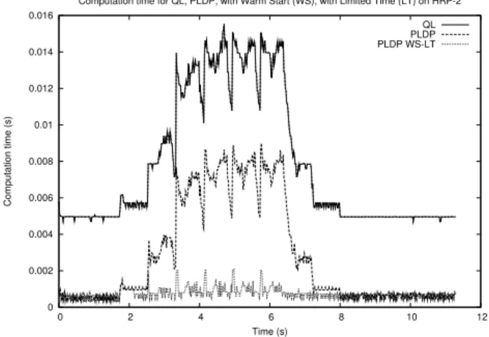
We naturally expect to gain n2 flops at each iteration thanks to the off-line change of variable. Furthermore, QL does not implement double sided inequality constraints like the ones we have in (19), so we need to double artificially the numbermof inequality constraints. Since computing the step α requires nm flops at each iteration and m ≈ n in our case, that’s a second n2 flops which we save with our algorithm. The mean computation time when using QL is 7.86 ms on the CPU of our robot, 2.81 ms when using our Primal Least Distance Problem (PLDP) solver. Detailed time measurements can be found in Fig. 1.
Even more interesting is the comparison with our warm start scheme combined with a limitation to two iterations for solving each QP. As discussed in section III-B, this generates short periods of sub-optimality of the solutions, but with no noticeable effect on the walking motions obtained in the end: this scheme works perfectly well, with a mean computation time of only 0.74 ms and, most of all, a maximum time less than 2 ms!
A better understanding of how these three options relate can be obtained from Fig. 2, which shows the number of constraints activated by QL for each QP, which is the exact number of active constraints. This figure shows then the difference between this exact number and the approximate number found by PLDP, due to the fact that we decided to never check the sign of the Lagrange multipliers. Most
0 0.002 0.004 0.006 0.008 0.01 0.012 0.014 0.016 0 2 4 6 8 10 12 Computation time (s) Time (s)
Computation time for QL, PLDP, with Warm Start (WS), with Limited Time (LT) on HRP-2 QL PLDP PLDP WS-LT
Fig. 1. Computation time required by a state of the art generic QP solver (QL), our optimized solver (PLDP), and our optimized solver with warm start and limitation of the computation time, over 10 seconds of experiments.
-10 -5 0 5 10 15 20 0 2 4 6 8 10 12 Activated Constraints Time (s)
Number of activated constraints QL, PLDP, with Warm Start (WS), with Limited Time (LT) QL PLDP PLDP WS-LT
Fig. 2. Number of active constraints detected by a state of the art solver (QL), difference with the number of active constraints approximated by our algorithm (PLDP), between 0 and 2, and difference with the approximation by our algorithm with warm start and limitation of the computation time, between -9 and 2.
often, the two algorithms match or PLDP activates only one constraint in excess. The difference is therefore very small. This difference naturally grows when implementing a maximum of two iterations for solving each QP in our warm starting scheme: when a whole group of constraints needs to be activated at once, this algorithm can identify only two of them each time a new QP is treated. The complete identifi-cation of the active set is delayed therefore over subsequent QPs: for this reason this algorithm appears sometimes to miss identifying as many as 9 active constraints, while still activating at other times one or two constraints in excess. Note that, regardless of how far we are from the real active set, the solution obtained in the end is always feasible.
VI. CONCLUSION
In this article we introduced an optimized algorithm for the fast solution of a particular QP in the context of LMPC for online walking motion generation. We discussed alternative methods for the solution of QPs, and analyzed how do their
properties reflect on our particular problem. Our algorithm was designed with the intension to use as much as possible data structures which are pre-computed off-line. In such a way, we are able to decrease the online computational complexity. We made a C++ implementation of our algorithm and presented both theoretical and numerical comparison with state of the art QP solvers. The issue of “warm-starting” in the presence of a real-time bound on the computation time was tested numerically, and we presented quantifiable results.
ACKNOWLEDGMENTS
This research was supported by the French Agence Na-tionale de la Recherche, grant reference ANR-08-JCJC-0075-01. This research was also supported by Research Council KUL: CoE EF/05/006 Optimization in Engineering Center (OPTEC). The research of Pierre-Brice Wieber was sup-ported by a Marie Curie International Outgoing Fellowship within the 7th European Community Framework Programme. Hans Joachim Ferreau holds a PhD fellowship of the Re-search Foundation - Flanders (FWO).
REFERENCES
[1] P.-B. Wieber, “Holonomy and nonholonomy in the dynamics of articulated motion,” in Proc. of the Ruperto Carola Symposium on Fast Motion in Biomechanics and Robotics,2005.
[2] S. Kajita, F. Kanehiro, K. Kaneko, K. Fujiwara, K. Harada, K. Yokoi, and H. Hirukawa, “Biped walking pattern generation by using preview control of zero-moment point,” in Proc. of the IEEE Int. Conf. on Robot. & Automat.,pp.1620-1626, 2003.
[3] P.-B. Wieber, “Trajectory free linear model predictive control for stable walking in the presence of strong perturbations,” inProc. of IEEE-RAS Int. Conf. on Humanoid Robots,pp.137-142, 2006.
[4] H. Diedam, D. Dimitrov, P.-B. Wieber, M. Katja, and M. Diehl, “Online walking gait generation with adaptive foot positioning through linear model predictive control,” inProc. of the IEEE/RSJ IROS,2008. [5] S. Wright, “Applying new optimization algorithms to model predictive
control,” inProc. of CPC-V, 1996.
[6] D. Dimitrov, J. Ferreau, P.-B. Wieber, and M. Diehl, “On the im-plementation of model predictive control for on-line walking pattern generation,” in Proc. of the IEEE Int. Conf. on Robot. & Automat., 2008.
[7] K. Schittkowski, “QL: A Fortran code for convex quadratic pro-gramming - User’s guide,” Department of Mathematics, University of Bayreuth, Report, Version 2.11, 2005.
[8] P.E. Gill, N.I. Gould, W. Murray, M.A. Saunders, and M.H. Wright “A weighted gram-schmidt method for convex quadratic programming,” Mathematical Programming,Vol.30, No.2, pp.176-195, 1984 [9] J. Nocedal, and S. J. Wright, “Numerical optimization,” Springer
Series in Operations Research, 2nd edition, 2000.
[10] R. A. Bartlett, A. W¨achter, and L. T. Biegler, “Active set vs. interior point strategies for model predictive control,” inProc. of the American Control Conference,pp.4229-4233, June, 2000.
[11] C. Rao, J. B. Rawlings, and S. Wright, “Application of interior point methods to model predictive control,”J. Opt. Theo. Applics.,pp. 723-757, 1998.
[12] I. Das, “An active set quadratic programming algorithm for real-time predictive control,”Optimization Methods and Software,Vol.21, No.5, pp.833-849, 2006.
[13] P.-B. Wieber, ”Viability and Predictive Control for Safe Locomotion”, Proceedings IEEE/RSJ International Conference on Intelligent RObots and Systems 2008.
[14] H.J. Ferreau, “An online active set strategy for fast solution of parametric quadratic programs with applications to predictive engine control,”University of Heidelberg,2006.
[15] R. Fletcher, “Practical Methods of Optimization,”John Wiley & Sons, 1981.