Equity Portfolio Diversification

NBER WORKING PAPER SERIES

EQUITY PORTFOLIO DIVERSIFICATION William N. Goetzmann

Alok Kumar Working Paper8686

http://www.nber.org/papers/w8686

NATIONAL BUREAU OF ECONOMIC RESEARCH 1050 Massachusetts Avenue

Cambridge, MA 02138 December 2001

We would like to thank K. Geert Rouwenhorst for helpful discussions and valuable comments. In addition, we would like to thank Itamar Simonson for making the investor data available to us and Terrance Odean for answering numerous questions about the investor database. The views expressed herein are those of the authors and not necessarily those of the National Bureau of Economic Research.

© 2001 by William N. Goetzmann and Alok Kumar. All rights reserved. Short sections of text, not to exceed two paragraphs, may be quoted without explicit permission provided that full credit, including © notice, is given to the source.

Equity Portfolio Diversification

William N. Goetzmann and Alok Kumar NBER Working Paper No. 8686

December 2001 JEL No. G0, G1, G2

ABSTRACT

In this paper we examine the portfolios of more than 40,000 equity investment accounts from a large discount brokerage during a six year period (1991-96) in recent U.S. capital market history. Using the historical performance for the equities in these accounts, we find that a vast majority of investors in our sample are under-diversified. Even accounting for the likelihood we have selected on speculators, the magnitude of the diosyncratic risk taken by investors in our sample is surprising. Investors are aware of the benefits of diversification but they appear to adopt a "naive" diversification strategy where they form portfolios without giving proper consideration to the correlations among the stocks. Over time, the degree of diversification among investor portfolios has improved but these improvements result primarily from changes in the correlation structure of the US equity market. Cross-sectional variations in diversification across demographic groups suggest that investors in low income and non-professional categories hold the least diversified portfolios. In addition, we find that young, active investors are over-focused and hold under-diversified portfolios. Overall, our results indicate that investors realize the benefits of diversification but they face a daunting task of "implementing" and maintaining a well-diversified portfolio.

William N. Goetzmann Alok Kumar

Yale University Cornell University

School of Management Department of Economics

and NBER Uris Hall

[email protected] Ithaca, NY 14853

I Introduction

U.S. equity risk has a large idiosyncratic component, much of which may be reduced through portfolio diversification. Virtually all asset pricing models posit that securities are priced by a diversified, marginal investor who demands little or no compensation for holding idiosyncratic risk. As a consequence, most rational models of investor choice suggest that investors hold diversified portfolios to reduce or eliminate non-compensated risk. But do they?

In this paper we examine the portfolios of more than 40,000 equity investment accounts

from a large discount brokerage during a six year period (1991-96) in recent U.S. capital market history. Using the historical performance for the equities in these accounts, we find that a vast majority of investors in our sample are under-diversified. Even accounting for the likelihood we have selected on speculators, the magnitude of the idiosyncratic risk taken by investors in our sample is surprising. Investors are certainly aware of the benefits of diversification. Over time, the average number of stocks in investor portfolios has increased and this has resulted in a decrease in the average portfolio variance. In addition, the average correlation among stocks in the US equity market has declined steadily over the 1991-96time period and that has led to a significant decrease in the variance of investor portfolios. However, over time, there is no decrease in either the excess average correlation (relative to benchmark portfolios) or the excess normalized variance. This suggests that investors adopt a “naive” diversification strategy where they form portfolios without giving proper consideration to the correlations among the stocks.

It is possible that investors do not diversify appropriately due to the small size of their portfolio. The inability of investors to buy in round lots and overall higher stock prices may prevent investors with smaller portfolios from diversifying. However, given that the mean portfolio size of investors in our sample is $35,629 (median is $13,869), these factors are less likely to be the dominant factors responsible for the observed lack of diversification

among investor portfolios. Clearly, investors that hold larger portfolios are more diversified and earn higher risk-adjusted performance but there is no evidence that investors that hold a larger number of stocks are able to reduce the variance of their portfolios through better stock selection. The average correlation among the stocks in portfolios containing a larger number of stocks is not lower than the average correlation among stocks in portfolios with fewer stocks. This indicates that investors with larger portfolios have better diversified portfolios merely because they hold a larger number of stocks and not due to any inherent superior portfolio composition skills.

One might argue that the investment accounts we are analyzing are “play money” accounts that people keep for gambling and entertainment purpose while the bulk of their actual invest-ment including retireinvest-ment money is elsewhere. This seems quite unlikely. At any given instant of time, the aggregate value of investor portfolios is approximately $2.5 billion. Furthermore, the average ratio of account size to annual income level is approximately 1.45 if maximum portfolio value is used as a measure of portfolio size and 0.79 if the average portfolio value is used as a measure of portfolio size. The portfolio size to income ratio is much higher for lower income groups. For example, this ratio is 3.62 for investors that earn less than $15,000 per year and 1.79 for investors with annual income between $20,000 and $30,000. So the money in the investment accounts do not represent an insignificant fraction of the entire household portfolio.

Turning to the cross-sectional differences in our sample, we find that the degree of diversifi-cation varies dramatically across investor accounts. Diversifidiversifi-cation level increases with income as well as age and this reflects an increasing degree of risk aversion with age and income. The degree of diversification also varies across occupation categories. Investors that belong to non-professional job categories (blue-collar workers, clerical workers and sales and service workers) hold the least diversified portfolios in our sample while investors who are retired are on the other end of the diversification spectrum where they hold the most diversified portfolios.

The cross-sectional variation in diversification across occupation categories further support the view that risk aversion may increase with age.

Overall, our results suggest that investors are unable to (or unwilling to) choose stocks in a judicious manner. They appear to adopt a “naive” diversification strategy where they hold portfolios with several stocks but without giving proper consideration to the correlations among the stocks they hold. These results are consistent with the findings of Rode (2000) who emphasizes the importance of “implementation” - investors may realize the benefits of diversification but they may face difficulty in implementing a well-diversified portfolio. As a result, investors may use simple “rules of thumb” to form their portfolios. The use of simple diversification heuristics has also been documented in Benartzi and Thaler (2001) who find that investors adopt a simple “1/n” rule when formulating their retirement-fund asset allocation

decisions.

So why do investors hold only a handful of stocks and why is the average correlation among stocks in their portfolios so high? Merton (1987) suggests that due to search and monitoring costs investors may limit the number of stocks in their portfolios. Investors may also develop a false perception that they can manage their portfolio risks better by a thorough understanding of a small number of firms rather than diversifying. Using survey data from a set of large and experienced investors, DeBondt (1998) finds that such a belief is quite common among investors. On the issue of why the average correlation among stocks in investor portfolios is high, previous studies have documented that investors appear to ignore correlations among stocks when forming their portfolios (Kroll, Levy, and Rapoport 1988), possibly due to the sequential nature of the portfolio formation process. Motivated by these experimental results, Shefrin and Statman (2000) develop a descriptive theory of portfolio choice where mental accounting (Thaler 1985) induces investors to form portfolios in a layered manner and the correlations among these layers are often ignored.

an “illusion of control” (Langer 1975). In experimental settings it has been observed that when factors such as involvement, choice and familiarity are introduced into chance situations, people become more confident and they start to believe that they can control the outcome of chance events. Investors may develop an illusory sense of control because they are directly involved in the investment process and they make their own choices instead of relying on others (as in the case of mutual funds) for their investment decisions. Familiarity with a certain set of stocks may further exacerbate the illusion of control where investors may fail to realize that more knowledge or more information does not necessarily imply control over the outcome (i.e., returns earned by the portfolio). Huberman (2001) finds that investors do indeed have a strong tendency to invest in stocks that they are familiar with. An illusion of control creates an inappropriate level of over-confidence and over-confident investors may mistakenly believe that they can earn superior performance by active trading and consequently they may choose not to diversify. As suggested in Kelly (1995), a sense of over-confidence can also emerge among investors simply because they may believe that their stock-picking abilities are superior to that of the market.

In our sample, we find that investors with higher monthly portfolio turnover rates (active investors) hold fewer stocks. Their portfolios have higher normalized portfolio variance and they eventually earn lower risk-adjusted returns. These results are consistent with the findings of Odean (1999) who documents that over-confident investors trade more actively and thus earn a lower net return. The lower level of diversification among active investors is another manifestation of investor over-confidence.

I.A Background: Household Investment Behavior

There is a considerable empirical literature on household investment choice. Beginning with Uhler and Cragg (1971), researchers have sought to understand the degree to which household asset allocation decisions conform to rational models of investor behavior. Blume and Friend

(1975) use tax filing and survey data to investigate diversification in household portfolios and find that the household portfolios are grossly under-diversified and the degree of diversification increases with wealth. In another study, Cohn, Lewellen, Lease, and Schlarbaum (1975) find that as wealth increases, a higher proportion of the total wealth is allocated to risky assets and investors exhibit decreasing relative risk aversion.

A number of authors recently have focused on the apparent under-investment in risky as-sets and explore possible explanatory factors. Guiso, Japelli, and Terlizze (1996) use Italian household survey data to test whether expected future borrowing constraints and exposure to non-diversifiable risks such as labor income risk (which may be reinforced by borrowing constraints) explain differences in equity holdings. Bertaut (1998) analyzes the stock mar-ket participation decisions of households and finds that the propensity to invest in equities is higher for investors with lower risk aversion, higher wealth and higher education because their information costs are lower. Heaton and Lucas (2000) study the asset holdings of investors who hold stocks and find that entrepreneurial stakes substitute for investment in equities. Consistent with these results, Gentry and Hubbard (2000) examine the portfolios of entre-preneurial households and find that their portfolios are grossly undiversified where more than 40% of their portfolios consist of active business assets. Perraudin and Sorensen (2000) suggest that frictions restrict the ability of investors to hold a large number of assets. Moskowitz and Vissing-Jorgensen (2001) provide further empirical evidence of improper diversification among households by examining their investments in private equity. They find that households hold concentrated portfolios of private equity even though private equity does not offer a better risk-return trade-off compared with a diversified portfolio of public equity.

Most of these previous studies use survey data which do not contain any information on the trading activities of households. In contrast, our dataset provides details of the composi-tion of investor portfolios and it contains a direct account of investor trades during a 6-year period. This allows us to measure the level of portfolio diversification accurately and more

importantly, the trading data allows us to examine the relationship between the behavior of undiversified investors and market returns. Our dataset does not contain information about the entire household portfolio and so we are unable to answer questions about the broader asset allocation decisions and the proportion held in risky assets. Instead, we are able to focus on the question of diversification within an asset class. It is important to point out that factors such as entrepreneurial risk or income exposure to particular industry risk factors can and should affect the selection of individual assets within the equity portfolio. In fact, Souleles (2001) has already shown that consumption risk, labor income risk, past returns as well as households’ expectations about future returns (i.e., their sentiment) are important determinants of house-holds’ portfolio composition and their buying decisions of risky assets. However, most income hedging arguments focus on systematic risk and neither of these important considerations is likely to convincingly explain long positions that include large idiosyncratic risk.

Our work is closest in spirit to Kelly (1995) who also examines equity portfolio diversifica-tion among households in the U.S. Using data from the 1983 Survey of Consumer Finances, she documents poor diversification among households. She finds that the median number of stocks in an investor portfolio is only two and less than one third of the households hold more than ten stocks. Our results are broadly consistent with the findings of Kelly (1995) and reinforce the evidence of poor diversification within a specific asset class documented in her study. We provide evidence of lack of diversification among investors in a different setting using a longer account of trading. In addition, we are able to develop a profile of diversified and undiversified investor groups using their trading characteristics, portfolio characteristics and demographic information. Furthermore, using the investor trading data, we are able to provide preliminary evidence in support of the hypothesis that idiosyncratic risk may be priced in equilibrium.

The rest of the paper is organized as follows: a brief description of the investor database and the sample used in the study is provided in Section II. In Section III we present the aggregate level diversification results and document the time variation in diversification among investors.

The cross-sectional variation in diversification across age, income and occupation categories is described in Section IV. In Section VI, we examine the asset pricing implications of portfolio diversification and estimate the strength of the contemporaneous relationship between the trading behavior of diversified and undiversified investor groups and market returns. We conclude in Section VI with a summary and a brief discussion.

II Data

The data for this study consists of trades and monthly portfolio positions of investors at a major discount brokerage house in the U.S. for the period of 1991-96. The database consists of three types of data files: (i) position files that contain the end-of-month portfolios of all investors, (ii) a trade file that contains all transactions carried out by the investors in the database, and (iii) a demographics file that contains information such as age, gender, marital status, income code, occupation code, geographical location (zip code), etc. for a subset of investors. There are a total of 77,995 households in the database of which 62,387 have traded in stocks. More

than half of the households in our database have 2 or more accounts. Approximately 27% of the households have 2 accounts, 13% have 3 accounts, 6% have 4 accounts and 6% have 5 or more accounts. All accounts for a given investor are combined to obtain a portfolio at the household level.

In addition to the investor database, we obtain monthly security prices and returns data from CRSP and use this data in combination with the position files to obtain a time series of monthly portfolio return for each household. These monthly portfolio return series are used to compute the various characteristics of investor portfolios.

Table I provides a summary of the key attributes of the investor database. The aggregate value of investor portfolios in our database is close to $2.5 billion at any given instant of time. An average investor holds a 4-stock portfolio (median is 3) with an average size of $35,629

(median is $13,869). Less than 10% of the investors hold portfolios over $100,000 and less than 5% of them hold more than 10 stocks. The average portfolio turnover rate which measures the frequency of trading is 7.59% (median is 2.53%) for our chosen sample. A typical investor makes less than 10 trades per year where the average trade size is $8,779 (median is $5,239). The average number of days an investor holds a stock is 187 trading days (median is 95).

Table II reports the 20 most widely held and 20 most actively traded stocks in our sample. It is clear that investor portfolios are heavily tilted towards stocks from technology and consumer companies. Household names such as IBM, Microsoft, General Motors, General Electric, Coca Cola, etc. dominate the list.

III Portfolio Diversification

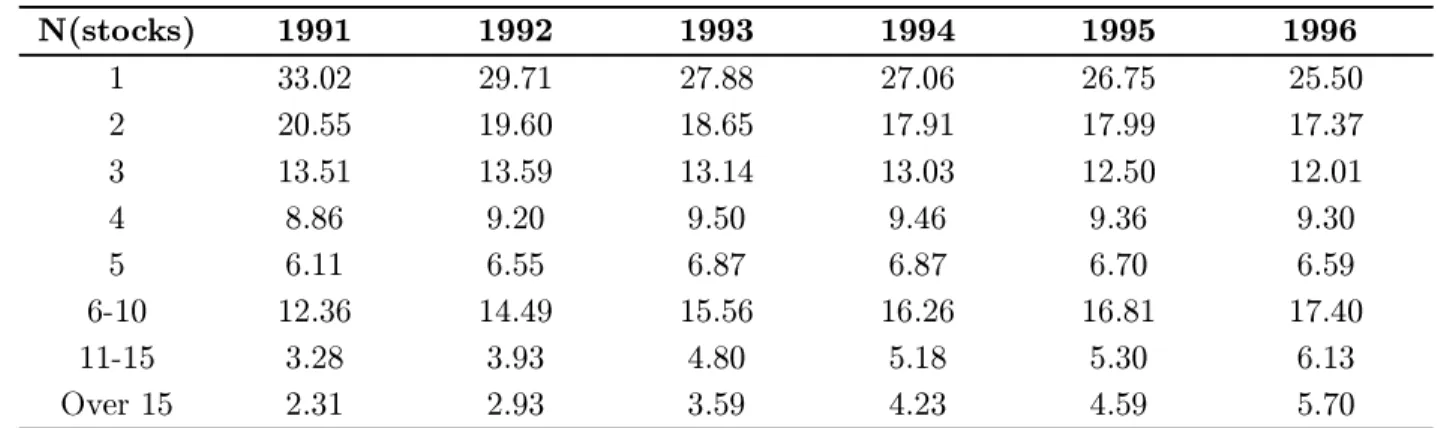
The observed degree of under-diversification among investor portfolios in our sample is quite surprising. More than 25% of investor portfolios contain only 1 stock and more than 50% of them contain fewer than 3 stocks. This pattern of holding concentrated portfolios is present throughout the 1991-96sample period though, over time, there has been an increase in the average number of stocks held by the investors (see Table III, Panel A). These results are boradly consistent with the findings of Blume and Friend (1975) and Kelly (1995). It is commonly believed that a well-diversified portfolio should consist of at least 10-15 stocks1. In

our sample, at any given monthly time-period, only 5-10% of the portfolios consist of more than 10 stocks.

It is possible that investors who hold relatively less diversified portfolios compensate for their lack of diversification by investing in mutual funds. However, we find that the average asset allocation to mutual funds is approximately 15% of the overall portfolio and more im-portantly, the allocation differences across diversification deciles are not significant. In other words, there is no evidence that investors with less diversified equity portfolios compensate

for their lack of diversification by investing more in mutual funds. Another possibility is that investors who are less diversified hold less risky stocks, i.e., they may disregard correlations among stocks and mistakenly belief that a collection of less risky stocks leads to a less risky portfolio. In our sample, we do not find any evidence of such diversification strategies. In fact, we find that less diversified investors hold riskier stocks. The mean standard deviation of stocks held by investors in the top and bottom diversification quartiles are 3.38% and 8.62% respectively.

In order to formally quantify the degree of under-diversification among the investor port-folios, we use three different (but related) measures of diversification. The first measure is a normalized version of the portfolio variance. The expected portfolio variance of an equal weighted portfolio withN stocks is defined as:

σ_p2 = 1_Nσ¯2+

_{N −1}

N

cov. (1)

where ¯σ2 is the average variance of all stocks in the portfolio and cov is the average covariance

among stocks in the portfolio. The normalized portfolio variance is obtained by dividing the portfolio variance by the average variance of stocks in the portfolio:

D1 =NVEWP= σ2_p ¯ σ2 = 1N + _{N −1} N covσ¯2 = 1_N +N −_N 1corr (2) where corr is the average correlation among stocks in the portfolio. We measure the portfolio variance in a normalized unit so that portfolios of different sizes can be aggregated. The expression for normalized variance clearly indicates that the portfolio variance can be reduced in two different ways. Firstly, it can be reduced by increasing the number of stocks in the portfolio (i.e., by increasingN) and secondly, it can be reduced by a proper selection of stocks

such that the average correlation among the stocks in the portfolio is lower. Variance reduction through proper stock selection reflects “skill” in portfolio composition while addition of stocks in the portfolio without lowering the average correlation is a reflection of a “naive” notion of

diversification2_{. In the limit, whenN → ∞, the portfolio variance (σ}2_{p) converges to the average}

covariance among the stocks in the portfolio (cov) and the normalized variance converges to 1. The degree of diversification can also be measured as the deviation of a portfolio from the market portfolio (Blume and Friend 1975). The weight of each security in the market portfolio is very small, so the diversification measure is approximately:

D₂=N i=1(wi− wm) 2 ₌N i=1(wi− 1 N_m)2 ≈ N i=1w 2 i (3)

where N is the number of securities held by the investor, N_m is the number of stocks in the

market portfolio, w_i is the portfolio weight assigned to stock i in the investor portfolio and w_m is the weight assigned to a stock in the market portfolio (w_m = 1/N_m). A lower value of D₂ is indicative of a higher level of diversification. Finally, we also use the number of stocks

in the portfolio as a “crude” measure of the degree of diversification:

D₃ =N. (4)

Each month, the expected return vector and the covariance matrix for the entire set of stocks traded by investors in our sample are estimated using past 5 years of monthly stock returns data3_{. These estimates are then used to compute the expected return, variance and}

average correlation among stocks for all investor portfolios. Table III (Panels B and C) report the normalized portfolio variance and the average correlation among stocks in investor portfo-lios. As expected, the normalized variance decreases as the number of stocks in the portfolio (N) increases. The normalized variance of concentrated portfolios is approximately 3-4 times

the normalized variance of well diversified portfolios. For example, in 1996, the normalized variance of well-diversified portfolios with 11-15 stocks is 0.163 while concentrated portfolios

with only 2 stocks on average have a normalized variance of 0.407.

2The idea of decomposing portfolio variance into two parts, one representing the effect of the number of stocks (_N) and the other representing the average correlation among the stocks in the portfolio (corr) is proposed in Goetzmann, Li, and Rouwenhorst (2001).

Over time, the normalized portfolio variance of investor portfolios has decreased but to a large extent due to changes in the correlation structure of the US equity market. The reduction in variance in the set of well-diversified portfolios is much larger than the variance improvement in the set of concentrated portfolios. For example, the normalized variance of 2-stock portfolios has improved from 0.508 in 1991 to 0.407 in 1996, a 20% decline. However,

during the same period, the normalized variance of portfolios containing more than 15 stocks has decreased from 0.291 to 0.130, a 55% decline. We also compute the average correlation

among the stocks in investor portfolios (see Table III, Panel C) and find that the average correlation among stocks in investor portfolios also decreases over time for portfolios of all sizes but the average correlation does not vary across portfolios at a given instant in time. The observed differences in average correlation are not statistically significant. This suggests that the reduction in portfolio variance during the 1991-96time-period occurs primarily from an increase in the number of stocks in the portfolio and not due to an improvement in the stock picking abilities of investors.

III.A Investor Portfolios Relative to Benchmark Portfolios

To better quantify the level of under-diversification among investor portfolios, we compare the investor portfolios with two simple benchmark portfolios, namely, the market portfolio and a large number of randomly chosen set of portfolios. Several sets of investor portfolios are formed, each set containing 1500 k-stock portfolios, where k = 2, . . . ,15. The average risk

characteristics of each of the random set of portfolios is compared with the average character-istics of matching investor portfolios. The market portfolio represents the risk-return trade-off the investors could have achieved with a passive trading style just by investing in one of the many available index funds. The set of random portfolios represents the risk-return trade-off a “naive” investor could have achieved by arbitrarily picking stocks. So these portfolios by no means constitute a “desirable” set but rather they represent the “minimum” level of risk-return

trade-off the investor portfolios should exhibit.

Figure 1 shows the positions of investor portfolios relative to the market portfolio (and the capital market line) in the mean-standard deviation (µ − σ) plane. Two monthly

time-periods are chosen in the first half of the sample period (February 1991 and June 1993) and two monthly time-periods are chosen in the second half of the sample period (September 1995 and June 1996). The past 5 years of monthly returns data is used to estimate the means and the standard deviations of the market portfolio and investor portfolios and the riskfree rate corresponds to the 90-day T-Bill rate.

We find that only a very small fraction of investor portfolios are above the capital market line (CML). In a month chosen in the first year of the sample period (February 1991), for instance, only 9.53% of the portfolios are above the CML and in a month in the last year of our sample (June 1996), 13.96% of the portfolios are above the CML. In other monthly time-periods also, only a small fraction of investor portfolios exhibit better risk-return trade-off than the market portfolio. Consistent with our previous results, we find that investor portfolios are more “spread out” in the µ − σ plane during the initial years but during the

latter years a relatively larger proportion of investors are closer to the CML though still only a small proportion of them are above the CML.

Comparing the variance of observed investor portfolios with the variance of randomly cho-sen portfolios, we again find that investor portfolios have relatively higher risk exposures. Figure 2 shows the average normalized variance of investor portfolios of different sizes rela-tive to the matching benchmark portfolios during the month of June 1996. The normalized variance of investor portfolios is approximately 25% higher than the normalized variance of benchmark portfolios and this difference increases with the size of the investor portfolio. This clearly indicates that the portfolios in our sample are not better than even those portfolios that in a sense provide a lower bound on the attainable risk-return trade-off.

III.B Diversification Over Time

During the 1991-96sample period, the average number of stocks in investor portfolios has increased almost monotonically from 4.19 in January 1991 to 6.51 in November 1996. The normalized portfolio variance has steadily decreased from 0.48 in January 1991 to 0.31 in November 1996(see Figure 3(a)). On surface, these two results seem to imply that the average diversification characteristics of investor portfolios have improved over time. However, when we compare investor portfolios with a benchmark of randomly chosen portfolios, we find that the risk exposure of investor portfolios are significantly higher than the benchmark portfolios and in fact, during the 1991-96period the extra normalized variance has increased from approximately 40% to 65%. So the improvements in investor portfolios result primarily from changes in the correlation structure of the equity market4. In Figure 4, we show the average correlation of both

investor portfolios and a set of randomly chosen portfolios. Clearly, the average correlation for both sets of portfolios decreases during the 1991-96time period but at each monthly time period, the average correlation among stocks in randomly chosen portfolios is significantly lower than the average correlation among stocks in actual investor portfolios.

In the analysis above we have combined portfolios of different sizes and find that at an aggregate level reduction in portfolio variance over time is driven primarily by changing market correlation structure. However, potential improvements in portfolio variance cross-sectionally are not revealed by this analysis. In Figure 5 we show the cross-sectional variation in average correlation across portfolios with different number of stocks for two monthly time-periods. The two monthly periods are chosen in the first and the last years of our sample period. For comparison, we also plot the average correlations of matched random portfolios. The procedure for constructing random portfolios is similar to the one described earlier. The average correlations of investor portfolios containingk-stocks and 1500 random portfolios with

4Malkiel and Xu (1997) report a similar finding by tracking the variation in correlations among industry portfolios during the 1970-95 time-period. They find that the mean correlation among the portfolios decreases over time thereby suggesting that the risk reduction benefits of holding a diversified portfolio has increased over time.

k-stocks are compared fork = 2, . . . ,15.

Three immediate observations can be made from the figure. First, the average correlations for both investor portfolios and random portfolios are lower in 9601 in comparison with 9101. This is consistent with our earlier result that portfolio variance decreases over time. Secondly, during both monthly time-periods, the average correlations of investor portfolios are higher than those of the random portfolios for all5 values of _k. The differences are statistically

significant for all values ofk(p-value<0.05). Finally, the average correlations decrease withk

for the set of random portfolios but for investor portfolios, the average correlations increase as

k increases. This suggests that portfolios of all sizes have worse diversification characteristics

than the benchmark portfolios and this result holds throughout our 6-year sample period. In Section IV, we investigate the cross-sectional variations in portfolio diversification in more detail.

III.C Diversification and Performance

Does better diversification translate directly into better portfolio performance? Figure 6shows the positions of concentrated portfolios (portfolios with 1-3 stocks) and relatively more diver-sified portfolios (portfolios with 7 or more stocks) relative to the market portfolio and the capital market line (CML) in the µ − σ plane. About 28% of portfolios that have 7 or more

stocks are above the CML while only 17% of concentrated portfolios are above the CML. The results are shown for one time period, namely September 1995, but similar results are obtained for other time periods. These are, of course, ex ante measures of portfolio performance. In

Figure 7 we plot the variation in realized risk-adjusted performance (measured using Sharpe Ratio) as the number of stocks in investor portfolios increase. There is a strong positive re-lationship between the degree of diversification and portfolio performance. Better diversified

5There is an exception. In 9601, for _k= 2, the average correlation of random portfolios is higher than that of investor portfolios.

portfolios earn higher risk-adjusted performance. To check the robustness of our results, we split the sample into two 3-year sub-periods and compute the portfolio performance separately for each of the two sub-periods. As shown in Figure 7, the strong positive relationship between diversification and performance is observed during both of the 3-year sub-periods. During the 1994-96sub-period, for instance, the average Sharpe ratio for 2-stock portfolios is 0.34 while portfolios with 15 or more stocks, on average, earn a Sharpe ratio of 0.56. Overall, better di-versification does translate into better risk-adjusted portfolio performance. However, investors can achieve these levels of performance by simply investing in one of the many available index funds.

IV Cross-Sectional Variation in Diversification

Having established that at an aggregate level investors are highly under-diversified, we now focus on the cross-sectional variation in diversification across investor portfolios. We investigate the role of relevant psychological factors in the portfolio formation decisions of investors and analyze diversification variation across various demographic groups to identify factors that can successfully explain the observed levels of under-diversification among investor portfolios.

IV.A Illusion of Control and Over-confidence

Investors may mistakenly believe that they can earn superior performance by active trading and consequently they may choose not to diversify their portfolios. If this hypothesis is true, investors with higher portfolio turnover rates are likely to be the less diversified group. Odean (1999) has already shown that over-confident investors trade more actively and as a result earn lower net returns. However, another manifestation of investor over-confidence is the lower level of diversification among the active group of investors. As discussed earlier, an inappropriate degree of over-confidence may arise from an illusory sense of control the investors may develop

due to their direct involvement in the investment process and due to their familiarity with a certain set of stocks. These factors are known to induce confidence among people in experi-mental settings (Langer 1975) and a similar behavioral mechanism may influence the portfolio formation decisions of investors in our sample.

Figure 8 shows how the degree of diversification varies with the frequency of trading. The second diversification measure, namely, the sum of squared portfolio weights (D2) is used to

measure the average diversification level and the monthly portfolio turnover rate is used to measure the frequency of trading. There is a strong positive relationship between D2 and

portfolio turnover rate. Portfolios in turnover deciles 1 and 2 have a D2 measure of 0.35

and 0.37 respectively while the top 2 turnover deciles have a D2 measure of 0.54 and 0.55

respectively. Note that a higher value of D2 implies a lower level of diversification. The

average number of stocks (D3 measure) in portfolios in the bottom 2 turnover deciles are 7.91

and 7.22 respectively while the average number of stocks in portfolios in the top 2 turnover

deciles are 5.38 and 5.05 respectively. Using Kolmogorov-Smirnov (KS) test6 we find that the

difference between the distributions of D2 and D3 for the bottom 2 turnover deciles and the

top 2 turnover deciles are statistically significant (p-value < 0.01). To test the robustness

of our results, we also compute the diversification measures across the turnover deciles for

6The Kolmogorov-Smirnov (KS) test (Press, Teukolsky, Vetterling, and Flannery 1992) is a non-parametric proce-dure that makes no assumptions about the underlying population distributions and compares the entire distribution instead of a distribution parameter. To compare two distributions (say SN1(x) and SN2(x)), the KS-test uses the

maximum value of the absolute difference between the two cumulative distributions as a test statistic:

Dobserved= max_−∞<x<∞ SN1(x)− SN2(x)

A large value of Dobserved provides a strong evidence against the null hypothesis of no difference between the two cumulative distributions. The significance level (p-value) of Dobserved is approximately given by:

Prob{Dactual> Dobserved}=QKS(Dobserved(

√ Ne+ 0.12 + 0√._N11 e)) where Ne= _NN1N2 1+N2 QKS(x) = 2 ∞ n=1( −1)(n−1)_e−2n2_x2 QKS(0) = 1, QKS(∞) = 0

the 1991-93 sub-period and the results are similar. As shown in the figure, the average D2

measure is higher for all turnover deciles during 1991-93 and this reflects the fact that investor portfolios are less diversified during the 1991-93 sub-period.

IV.B Diversification and Demographics

To identify the main factors that may be responsible for the observed levels of under-diversification among the investors in our sample, we analyze the variations in diversification across three demographic variables: (i) age, (ii) occupation, and (iii) income. Previous studies have es-tablished that risk aversion increases with age7 and wealth. If this is indeed true, portfolio

diversification (an indirect indicator of an investor’s risk aversion) must increase with age and income. In addition, if occupation and income are proxies for the amount of information (and education) investors have, an analysis of cross-sectional variations can reveal if better informed investors hold better diversified portfolios. More importantly, having shown earlier that there exists a strong relationship between the level of diversification and portfolio performance, our results from this section can help us target the investor groups that are likely to suffer the most from the lower levels of diversification.

Age

Figure 9 shows the relationship between diversification and age during the 1991-93 and the 1994-96periods. The degree of diversification increases with age during both the sub-periods. The average D2 diversification measure for investors in the age group of 26-36 (the

bottom age decile) is 0.53 during the 1994-96sub-period while the averageD2 is only 0.42 for

the top age decile which consists of investors in the age group of 70-82. Using the Kolmogorov-Smirnov test we find that the distributions of D2 for the top and bottom age deciles are

7King and Leape provide an alternative explanation. They suggest a life-cycle hypothesis of diversification where the portfolio diversification increases with age because with experience, investors acquire more information about the market.

significantly different from one other (p-val < 0.01). Other diversification measures yield

similar results. For instance, the average number of stocks (D3 measure) is 4.69 for the

bottom decile and 6.65 for the top decile during the 1994-96 sub-period. Overall, there is a strong positive relationship between age and the degree of diversification.

In order to understand better why diversification increases with age, we investigate the relationship between age and the frequency of trading. Are younger people less diversified because of their higher level of over-confidence? We find that the trading frequency decreases with age. The portfolio turnover rate is 6.82% for the bottom age decile (age between 26-36) and 5.02% for the top age decile (age between 70-82). The difference between the turnover distributions of the two groups is statistically significant (p-value <0.01). This suggests that

young, active investors are over-focused and hold concentrated and under-diversified portfolios.

Occupation

To investigate the variations in diversification across occupation, we form three broad occu-pation categories, namely, (i) professional category, consisting of investors that hold technical or managerial positions, (ii) non-professional category, consisting of investors who are either blue-collar workers, sales and service workers or clerical workers, and finally, (iii) the retired category. Other occupation codes such as student, housewife, etc. exist in our sample but given the small sizes of these groups, we do not include them in our analyses.

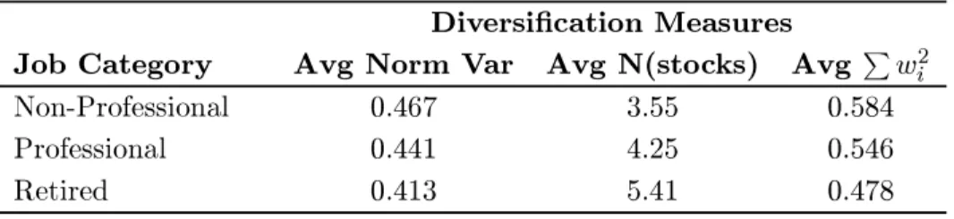
Table IV reports the average diversification measures for the 3 broad occupation categories during the 1991-93 and the 1993-96sub-periods. During both sub-periods, we find that the non-professional category holds the least diversified portfolios while investors in the retired fall on the other end of the diversification spectrum. For example, during the 1994-96sub-period, investors in the non-professional category hold 4.56stocks (the average normalized variance is 0.356) on average while investors in the retired category hold 6.89 stocks (the average normalized variance is 0.302). Using the Kolmogorov-Smirnov test we find that the

distributions of the 3 diversification measures for the non-professional and retired categories are significantly different from one other (p-value < 0.01). The average diversification level

of investor portfolios in the professional category falls in between the average diversification level of non-professional and retired categories and again, the differences in distributions are statistically significant (p-value <0.01).

As shown earlier, there is a positive relationship between the degree of diversification and performance. Consistent with our earlier results, we find that the average risk-adjusted performance (Sharpe ratio) during the 1991-96period for the non-professional category has the lowest value (0.321) and it is highest for the retired category (0.398). The Sharpe ratio

for the professional category is 0.373. The performance differences between these 3 categories

are statistically significant at 0.05 level.

Income

The third demographic variable we consider is income. We investigate the variations in diver-sification across different income categories because income may be a proxy for information or education level. We divide investors into 3 broad income groups: (i) low income category: the annual income is less than $30,000, (ii) medium income category: the annual income is between $ 40000 and $ 75,000, and (iii) high income category: the annual income is above than $75,000. Table V reports the average diversification measures for these 3 income categories during 1991-93 and 1993-96sub-periods. During the 1991-93 sub-period, the diversification differences across income categories are not statistically significant. However, during the 1994-96sub-period, the degree of diversification is higher for the high income category. The low income category holds on average of 4.71 stocks while the average number of stocks held by investors in the high income category is 5.84. Using the Kolmogorov-Smirnov test we find that the distributions of low income and high income categories are significantly different from each other (p-val < 0.01). Other diversification measures show a similar variation and yield

statistically significant differences.

IV.C Regression Results

Our results so far suggest that degree of portfolio diversification varies cross-sectionally across age, occupation and income. To measure the relative impact of age, income and occupation on the degree of portfolio diversification, we estimate a regression specification with dummy variables where we control for both portfolio size and trading frequency (portfolio turnover rate). The functional specification estimated is:

DIVi = b0+bps(PortfSizei) +bpt(PortfTurnoveri) +ba(Agei)

+ bid1(IncDummy1i) +bid2(IncDummy2i)

+ bjd1(JobDummy1i) +bjd2(JobDummy2i) +i (5)

Here, DIV is the portfolio diversification measure (normalized portfolio variance), PortfSize

variable measures the size of investor portfolios, PortfTurnover is the monthly turnover rate (the mean of monthly buy and sell turnover rates) which measures the frequency of trading, and Age is the age of the head of the household. The two income dummy variables, IncDummy1 and IncDummy2, correspond to the low and high income categories. Finally, JobDummy1 and JobDummy2 are the dummy variables for the non-professional and the retired occupation categories respectively.

The regression results are reported in Table VII. The sample is split into two sub-periods, 1991-93 and 1994-96, and the regression coefficients are estimated for each of these two 3-year sub-periods. During the 1991-93 sub-period, the coefficients are positive and statistically significant for PortfTurnover, IncDummy1 and JobDummy1 and negative and significant for PortfSize, Age, and JobDummy2. During the 1994-96sub-period, this sign pattern for the coefficient estimates is maintained. The coefficient of IncDummy2 is positive but insignificant during the 1991-93 sub-period but negative and significant during the 1994-96sub-period.

These regression results reinforce the results documented earlier. The coefficient estimate of PortfSize has a negative sign which suggests that the normalized variance is lower for larger portfolios, i.e., larger portfolios are better diversified. In Figure 8 we illustrated a negative relationship between the degree of portfolio diversification and trading frequency. A positive coefficient for the PortfTurnover variable confirms this earlier result. Investors who trade more often hold relatively less diversified portfolios. The coefficient for the Age variable is negative and this supports the result in Figure 9 where we illustrate a positive relationship between age and diversification.

The effect of income on diversification is captured by the two income dummy variables. A positive value for the coefficient of IncDummy1 suggests that low income investors have higher portfolio variance relative to the medium income investors and hence they are less diversified. In contrast, the coefficient on the dummy variable for high income (IncDummy3) is negative which suggests that high income investors hold more diversified portfolios relative to the medium income group investors.

Finally, we find that the coefficients of JobDummy1 is positive and significant while the coefficient of JobDummy2 is negative and significant during both the sub-periods. This pro-vides evidence that investors in both professional and retired categories hold better diversified portfolios compared with the non-professional category. Furthermore, the group of retired investors hold the most diversified portfolios.

V Trading Behavior of Investor Groups and Market Returns

In order to analyze the impact of trading behavior of investor groups on asset prices, we first classify investors into diversified and undiversified groups using the average correlation between stocks in the portfolio as a measure of diversification. The investors in the bottom quartile are identified as diversified while those in the top quartile are identified as undiversified. The

remaining investors are identified as unclassified. Next, we construct a daily and a monthly buy-sell imbalance (BSI) time-series for diversified and undiversified investor groups. The normalized buy-sell imbalance for time-periodt is defined as:

BSIt= _Nbt i=1V Bit−Ni=1stV Sit _Nbt i=1V Bit+Ni=1stV Sit (6) where

Nbt = Number of stocks purchased by the investor group during time-periodt, Nst = Number of stocks sold by the investor group during time-periodt, V B_it = Buy volume of stocki during time-periodt, and

V S_it = Sell volume for stockiduring time-periodt.

The strength of the contemporaneous relationship between flows and market returns is esti-mated using the following regression specification:

rmt=α+β_u(BSI_ut) +β_d(BSI_dt) +_t t= 1,2, . . . , T (7)

Here,r_mtis the return of the market in periodt, BSI_ut is the buy-sell imbalance in periodtfor

the undiversified investor group, BSIdt is the buy-sell imbalance in periodtfor the diversified

investor group, and_t is the error term.

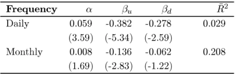
The contemporaneous relationship is estimated using both daily and monthly BSI time-series. The regression results are reported in Table VII (Panel A). At the monthly frequency, both the coefficients, β_u and β_d, are negative (β_u = −0.136, β_d = −0.062). However, only

one of the coefficients, namely, β_u, is statistically significant (t-values are −2.83 and −1.22

respectively). Qualitatively similar results are obtained when the regression specification is estimated using daily data. At the daily frequency, again, both the coefficients, β_u and β_d,

are negative (β_u =−0.382, β_d =−0.278) and both the coefficients are statistically significant

(t-values are −5.34 and −2.59 respectively).

The evidence that both coefficients, β_u and β_d, are negative at daily as well as monthly

contrar-ians. This is consistent with the findings of other recent studies that have used the investor database8. More importantly, we find that _{βu> βd}and the magnitude of the_t-value for β_u is larger than the magnitude of thet-value forβ_d. This suggests that the trading behavior

of undiversified investors is more strongly correlated with the market returns. To test the robustness of our results, we divide the 6-year sample period into two 3-year sub-periods and estimate the strength of contemporaneous relationship between flows and market returns in each of the two sub-periods. The results are reported in Table VII (Panels B and C). Once again, we find that β_u <0, β_d<0, β_u > β_d, and t_u > t_d for both the sub-periods

and at both daily and monthly frequencies.

These results suggest that the trading behavior (measured using BSI) of the group of undiversified investors is more strongly correlated with the market returns and the group of undiversified investors is likely to be the more salient of the two investor groups. The salience of the undiversified group of investors provide support to recent studies (Goyal and Santa-Clara 2001, Malkiel and Xu 2002) that posit that idiosyncratic risk is priced in equilibrium.

VI Summary and Conclusion

An examination of the portfolios of more than 40,000 equity investment accounts from a large

discount brokerage during a six year period (1991-96) in recent U.S. capital market history revealed that a vast majority of investors are under-diversified. Over time, the degree of diversification among investor portfolios has improved but these improvements result primarily from changes in the correlation structure of the US equity market. Investors are certainly aware of the benefits of diversification but they appear to adopt a “naive” diversification strategy where they hold portfolios with several stocks but without giving proper consideration to the correlations among the stocks. In addition to the lack of proper diversification that results

8Barber and Odean (2001), Hirshleifer, Myers, Myers, and Teoh (2002), and Hong and Kumar (2002) document that individual investors behave as contrarians around different types of public announcement events and market-wide news events.

from inappropriate stock selection, investor hold under-diversified portfolios due to an illusory sense of control which makes them over-confident. A significant group of investors in our sample believe that they can earn superior performance by active trading and consequently they choose not to hold well-diversified portfolios. Cross-sectional variations in diversification across demographic groups suggest that investors in low income and non-professional categories hold the least diversified portfolios. In addition, we find that young, active investors are over-focused and they are more inclined to hold under-diversified portfolios. Analyzing the relationship between the trading behavior of investor groups and market returns, we find that the trading behavior of the group of undiversified investors is more strongly correlated with the market returns and hence, the undiversified investor group is likely to be the more salient of the two investor groups. Overall, our results indicate that investors realize the benefits of diversification but they face a daunting task of “implementing” and maintaining a well-diversified portfolio.

What implications do the widespread presence of under-diversified portfolios have for asset-pricing? If investors diversify “naively”, they may falsely believe that they hold diversified portfolios and as a result the perception of market risk will vary across investors. Consequently, investors are likely to demand different amounts of risk compensation for holding stocks, in accordance with their heterogeneous but mistaken beliefs. If the degree of under-diversification among the investors in our sample is a good representation of the level of diversification among the investor population in the market, asset-pricing models should be calibrated to take into account the level of under-diversification among the investor population. Empirical results have already started to emerge (Goyal and Santa-Clara 2001, Malkiel and Xu 2002) which suggest that idiosyncratic risk is in fact priced in equilibrium.

References

Barber, Brad, and Terrance Odean, 2001, All that glitters: The effect of attention and news on the buying behavior of individual and institutional investors, Working Paper, Haas School of Business, University of California at Berkeley, November 2001.

Benartzi, Shlomo, and Richard H. Thaler, 2001, Naive diversification strategies in retirement saving plans, American Economic Review 91, 79—98.

Bertaut, Carol C., 1998, Stockholding behavior of us households: Evidence from 1983-1989 survey of consumer finances, Review of Economics and Statistics 80, 263—275.

Blume, Marshall E., and Irwin Friend, 1975, The asset structure of individual portfolios and some implications for utility functions, Journal of Finance 30, 585—603.

Cohn, Richard A., Wilbur G. Lewellen, Ronald C. Lease, and Gary G. Schlarbaum, 1975, Individual investor risk aversion and investment portfolio composition, Journal of Finance 30, 605—620.

DeBondt, Werner, 1998, A portrait of the individual investor, European Economic Review 42, 831—844.

Gentry, William M., and R. Glenn Hubbard, 2000, Entrepreneurship and household saving, Working Paper, Columbia Business School, July 2000.

Goetzmann, William N., Lingfeng Li, and K. Geert Rouwenhorst, 2001, Long-term global market correlations, Working Paper International Center for Finance, Yale School of Man-agement, May 2001.

Goyal, Amit, and Pedro Santa-Clara, 2001, Idiosyncratic risk matters, Working Paper, An-derson Graduate School of Management, UCLA, November 2001.

Guiso, L., T. Japelli, and D. Terlizze, 1996, Income risk, borrowing constraints and portfolio choice, American Economic Review 86, 158—172.

Heaton, John, and Deborah Lucas, 2000, Portfolio choice and asset prices: the importance of entrepreneurial risk, Journal of Finance 55, 1163—1198.

Hirshleifer, David A., James N. Myers, Linda A. Myers, and Siew H. Teoh, 2002, Do individual investors drive post-earnings announcement drift?, Working Paper, January 2002.

Hong, Dong, and Alok Kumar, 2002, What induces noise trading around public announcement events?, Working Paper, Department of Economics, Cornell University, February 2002. Huberman, Gur, 2001, Familiarity breeds investment, Review of Financial Studies 14, 659—680. Kelly, Morgan, 1995, All their eggs in one basket: Portfolio diversification of us households,

Journal of Economic Behavior and Organization 27, 87—96.

King, Mervyn, and Jonathan Leape, 1987, Asset accumulation, information and life cycle, Journal of Financial Economics 29, 97—112.

Kroll, Yoram, Haim Levy, and Amnon Rapoport, 1988, Experimental tests of the separation theorem and the capital asset pricing model, American Economic Review 78, 500—519. Langer, Ellen J., 1975, The illusion of control, Journal of Personality and Social Psychology

32, 311—328.

Malkiel, Burton G., and Yexiao Xu, 1997, Risk and return revisited, Journal of Portfolio Management 23, 9—14.

, 2002, Idiosyncratic risk and security returns, Working Paper, School of Management, University of Texas at Dallas, January 2002.

Merton, Robert C., 1987, A simple model of capital market equilibrium with incomplete in-formation, Journal of Finance 42, 483—510.

Moskowitz, Tobias J., and Annette Vissing-Jorgensen, 2001, The returns to entrepreneurial investment: A private equity premium puzzle?, American Economic Review Forthcoming.

Odean, Terrance, 1999, Do investors trade too much?, American Economic Review 89, 1279— 1298.

Perraudin, W.R.M., and Bent E. Sorensen, 2000, The demand for risky assets: Sample selection and household portfolios, Journal of Econometrics 97, 117—144.

Press, William H., Saul A. Teukolsky, William T. Vetterling, and Brian P. Flannery, 1992, Numerical Recipes in C: The Art of Scientific Computing, Second Edition (Cambridge Uni-versity Press, Cambridge, UK.).

Rode, David, 2000, Portfolio choice and perceived diversification, Working Paper, Department of Social and Decision Sciences, Carnegie Mellon University.

Shefrin, Hersh M., and Meir Statman, 2000, Behavioral portfolio theory, Journal of Financial and Quantitative Analysis 35, 127—151.

Souleles, Nicholas S., 2001, Household portfolio choice, transaction costs, and hedging motives, Working Paper, Wharton School, University of Pennsylvania, September 2001.

Statman, Meir, 1987, How many stocks make a diversified portfolio?, Journal of Financial and Quantitative Analysis 22, 353—363.

Thaler, Richard H., 1985, Mental accounting and consumer choice, Marketing Science 4, 199— 214.

Uhler, R.S., and J.G. Cragg, 1971, The structure of the asset portfolios of households, Review of Economic Studies 38, 341—357.

Table I

The Investor Database

This table summarizes the characteristics of the households in our sample. The primary dataset consists of trades and monthly portfolio positions of investors at a major discount brokerage house in the U.S. for the period of 1991-96. The database consists of three types of data files: (i) position files that contain the end-of-month portfolios of all investors, (ii) a trade file that contains all transactions carried out by the investors in the database, and (iii) a demographics file that contains information such as age, gender, marital status, income code, occupation code, geographical location (zip code), etc. for a subset of investors.

Time Period: Jan. 1991 - Nov. 1996.

Pane

l A: Households

Number of households: 79,995

Number of accounts: 158,031

Number of households with position in equities: 62,387

Number of households with 5 or more trades: 41,039

Panel B: Household Characteristics

Aggregate value of investor portfolios in a typical month: $2.48 billion

Average size of investor portfolios: $35,629 (Median = $13,869)

Average number of trades: 41 (Median = 19)

Average number of stocks in the portfolio: 4 (Median = 3)

Average age of the household: 50 (Median = 48)

Panel C: Securities

Total number of traded common stocks: 10,486

Number of common stocks for which data is available from CRSP: 9,893

Panel D: Trades

Total number of trades: 2,886,912

Number of trades in common stocks: 1,854,776

Number of trades in common stocks executed by the households: 1,677,547

Number of trades in stocks traded on NYSE, NASDAQ and AMEX: 1,546,016

Average Portfolio Turnover: 7.59% (Median: 2.53%)

Table II

Most Widely Held and Most Actively Traded Stocks in our Investor Database

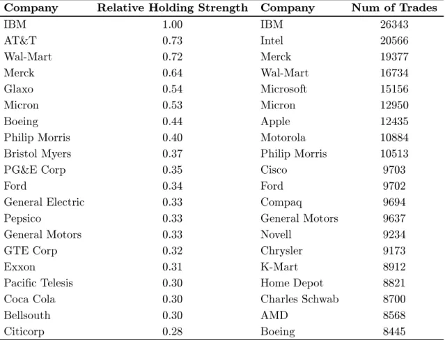
This table reports (a) 20 most widely held stocks and (b) 20 most actively traded stocks in our investor database. The relative holding strength is computed using the end of month portfolio position data.

Company

Relative Holding Strength Company

Num of Trades

IBM 1.00 IBM 26343 AT&T 0.73 Intel 20566 Wal-Mart 0.72 Merck 19377 Merck 0.64 Wal-Mart 16734 Glaxo 0.54 Microsoft 15156 Micron 0.53 Micron 12950 Boeing 0.44 Apple 12435

Philip Morris 0.40 Motorola 10884

Bristol Myers 0.37 Philip Morris 10513

PG&E Corp 0.35 Cisco 9703

Ford 0.34 Ford 9702

General Electric 0.33 Compaq 9694

Pepsico 0.33 General Motors 9637

General Motors 0.33 Novell 9234

GTE Corp 0.32 Chrysler 9173

Exxon 0.31 K-Mart 8912

Pacific Telesis 0.30 Home Depot 8821

Coca Cola 0.30 Charles Schwab 8700

Bellsouth 0.30 AMD 8568

Table III

Aggregate Level Diversification Characteristics of Investor Portfolios

This table summarizes the aggregate level diversification characteristics of investor portfolios over time. The normalized variance and the average correlation of the portfolios are estimated using past 5 years of monthly returns data. The normalized variance of a portfolio is defined as:

NVEWP= σ 2 p ¯ σ2 = 1_N + N −1 N covσ¯2 = 1_N +N −_N 1corr where corr is the average correlation among the stocks in the portfolio.

Panel A: Percent of Portfolios

N(stocks)

1991

1992

1993

1994

1995

1996

1 33.02 29.71 27.88 27.0626.75 25.50 2 20.55 19.60 18.65 17.91 17.99 17.37 3 13.51 13.59 13.14 13.03 12.50 12.01 4 8.869.20 9.50 9.469.36 9.30 5 6.11 6.55 6.87 6.87 6.70 6.59 6-10 12.3614.49 15.5616.2616.81 17.40 11-15 3.28 3.93 4.80 5.18 5.30 6.13 Over 15 2.31 2.93 3.59 4.23 4.59 5.70

Panel B: Normalized Portfolio Variance

N(stocks)

1991

1992

1993

1994

1995

1996

2 0.645 0.612 0.601 0.589 0.570 0.563 3 0.508 0.470 0.459 0.443 0.417 0.407 4 0.441 0.397 0.385 0.366 0.337 0.329 5 0.3960.347 0.338 0.322 0.293 0.278 6-10 0.355 0.300 0.291 0.267 0.234 0.218 11-15 0.309 0.2460.239 0.217 0.182 0.163 Over 15 0.291 0.224 0.220 0.192 0.151 0.130

Panel C: Average Correlation among Stocks in the Portfolio

N(stocks)

1991

1992

1993

1994

1995

1996

2 0.323 0.251 0.228 0.203 0.160 0.146 3 0.312 0.250 0.231 0.203 0.157 0.143 4 0.314 0.251 0.233 0.202 0.154 0.143 5 0.314 0.2460.231 0.202 0.158 0.139 6-10 0.325 0.259 0.245 0.210 0.161 0.139 11-15 0.329 0.260 0.249 0.214 0.165 0.140 Over 15 0.341 0.271 0.264 0.224 0.168 0.143

Table IV

Diversification across Occupation Categories.

This table reports the three diversification measures for the three broad occupation categories. The non-professional category consists of blue-collar workers, sales and service workers, and clerical workers while the professional job category includes investors who hold technical and managerial positions. The three diversification measures reported are: (i) the normalized portfolio variance, (ii) the average number of stocks in a portfolio, and (iii) the sum of the squared portfolio weights.

Panel A: Time Period: 1991-93

Diversification Measures

Job Category

Avg Norm Var Avg N(stocks) Avg

w2 i

Non-Professional 0.467 3.55 0.584

Professional 0.441 4.25 0.546

Retired 0.413 5.41 0.478

Panel B: Time Period: 1994-96

Diversification Measures

Job Category

Avg Norm Var Avg N(stocks) Avg

w2 i

Non-Professional 0.3564.560.530

Professional 0.324 5.57 0.479

Table V

Diversification across Income Levels.

This table reports the three diversification measures for the three broad income categories. The three diversification measures are: (i) the normalized portfolio variance, (ii) the average number of stocks in a portfolio, and (iii) the sum of the squared portfolio weights.

Panel A: Time Period: 1991-93

Diversification Measures

Income Level

Avg Norm Var Avg N(stocks) Avg

w2 i

Low (Less than 40,000) 0.431 4.33 0.547

Medium (40,000 - 75,000) 0.442 4.22 0.540

High (Above 75,000) 0.447 4.24 0.551

Panel B: Time Period: 1994-96

Diversification Measures

Income Level

Avg Norm Var Avg N(stocks) Avg

w2 i

Low (Less than 40,000) 0.335 4.71 0.523

Medium (40,000 - 75,000) 0.317 5.45 0.485

Table VI

Determinants of Degree of Diversification

This table reports the results from the following pooled regression with dummy variables: DIVi = b0+bps(PortfSizei) +bpt(PortfTurnoveri) +ba(Agei)

+ bid1(IncDummy1i) +bid2(IncDummy2i) + bjd1(JobDummy1i) +bjd2(JobDummy2i) +i

DIV is the portfolio diversification measure (normalized portfolio variance), PortfSize variable measures

the size of investor portfolios, PortfTurnover is the monthly turnover rate (the mean of monthly buy and sell turnover rates) which measures the frequency of trading, and Age is the age of the head of the household. The two income dummy variables, IncDummy1 and IncDummy2, correspond to the low and high income categories. Finally, JobDummy1 and JobDummy2 are the dummy variables for the non-professional and the retired occupation categories respectively.

N = 9797,R¯2 = 0_.0458 _N = 56 32_,R¯2= 0_.0451

1991-93 1994-96

Variable Coefficient t-value Coefficient t-value

Intercept 6.29 45.21 5.94 32.66

Portfolio Size -0.013 -11.77 -0.010 -8.64

Portfolio Turnover 0.507 12.01 0.554 9.12

Investor Age -0.254 -9.55 -0.239 -6.72

Income: Less than 40,000 1.537 2.48 2.722 1.94

Income: More than 75,000 0.210 0.33 -1.245 -1.96

Occupation: Non-Professional 3.019 3.37 3.859 3.22

Table VII

Trading Behavior of Diversified and Undiversified Investor Groups and Market Returns

This table reports the results from the following regression:

rmt=α+β_u(BSI_ut) +β_d(BSI_dt) +_t t= 1,2, . . . , T

r_mtis the return of the market in periodt, BSI_utis the buy-sell imbalance in periodtfor the undiversified

investor group, BSIdtis the buy-sell imbalance in periodtfor the diversified investor group, and_t is the

error term. Using the average correlation between stocks in the portfolio as a measure of diversification, the investors in the top diversification quartile are identified as diversified while those in the bottom diversification quartile are identified as undiversified. Panel A reports the results for the entire 1991-96 sample period while Panels B and C report the coefficient estimates for the two sub-samples, 1991-93 and 1994-96, respectively.

Panel A: Time Period: 1991-96

Frequency

α βu βd R¯2

Daily 0.059 -0.382 -0.278 0.029

(3.59) (-5.34) (-2.59)

Monthly 0.008 -0.136-0.062 0.208

(1.69) (-2.83) (-1.22)

Panel B: Time Period: 1991-93

Daily 0.065 -0.387 -0.209 0.026

(2.42) (-3.52) (-1.92)

Monthly 0.006-0.165 -0.051 0.208

(0.66) (-2.39) (-0.60)

Panel C: Time Period: 1994-96

Daily 0.056-0.375 -0.256 0.029

(2.65) (-4.00) (-1.69)

Monthly 0.011 -0.123 -0.063 0.145

Figure 1

Investor Portfolios Relative to the Market Portfolio

This figure shows the positions of investor portfolios relative to the market portfolio (and the Capital Market Line). Two monthly time-periods are chosen in the first half of the sample period (February 1991 and June 1993) and two of them are chosen in the second half of the sample period (September 1995 and June 1996). The past 5 years of monthly returns data is used to estimate the means and the standard deviations of the market portfolio and investor portfolios. The riskfree rate corresponds to the 90-day T-Bill rate. 0 5 10 15 20 −5 0 5 Mkt Portf Rf Capital Mkt Line

Exp Monthly Ret (%)

Time Period: 9102 Investors above CML = 9.53% 0 5 10 15 20 −5 0 5 Time Period: 9306 Investors above CML = 10.55% 0 5 10 15 20 −5 0 5 Monthly Std Dev (%)

Exp Monthly Ret (%)

Time Period: 9509 Investors above CML = 20.15% 0 5 10 15 20 −5 0 5 Monthly Std Dev (%) Time Period: 9606 Investors above CML = 13.96%

Figure 2

Variance of Investor Portfolios Relative to a Set of Randomly Chosen Portfolios

This figure shows the normalized variance of actual investor portfolios and 1500 randomly chosen port-folios (the benchmark portport-folios) during the month of June 1996. Similar results are obtained for other months during our 1991-96 sample period.

0 2 4 6 8 10 12 14 16 0 0.1 0.2 0.3 0.4 0.5 0.6 0.7

Average Number of Stocks in the Portfolio

Normalized Variance

Time Period: 9606

Actual Investor Portfolios

Figure 3

Diversification over Time

The figure shows the variations in investor portfolio characteristics over time. The top figure shows the average number of stocks in investor portfolios and the normalized variance of their portfolios over time while the bottom figure shows the extra variance taken by the investor portfolios relative to a set of randomly chosen portfolios.

Jan 91 Jan 92 Jan 93 Jan 94 Jan 95 Jan 96 3 3.5 4 4.5 5 5.5 6 6.5 7

Num of Stocks in the Portfolio

0.25 0.3 0.35 0.4 0.45 0.5

Normalized Variance of EWP

Jan 91 Jan 92 Jan 93 Jan 94 Jan 95 Jan 96 30 35 40 45 50 55 60 65 70 75 80

Time (Jan 1991 − Nov 96)

Extra Norm. Var. (in Percent)

Norm Var Num of Stocks

Figure 4

Correlation Structure of the US Equity Market Over Time

This figure shows the variation in the correlation structure of the US equity market during the 1991-96 time period. Each month 2000 portfolios containing upto 10 stocks are formed by selecting stocks ran-domly from the available list of stocks. Using the historical monthly returns data the portfolio correlation matrix is estimated and the average correlation among the stocks in the portfolio is computed. Finally, the average correlation for the month is obtained by taking the average across the 2000 randomly chosen portfolios. The monthly average correlations are also computed using the actual investor portfolios.

Jan 91 Jan 92 Jan 93 Jan 94 Jan 95 Jan 96

0 0.05 0.1 0.15 0.2 0.25 0.3 0.35 0.4

Time (Jan 1991 − Nov 1996)

Average Correlation

Randomly Chosen Portfolios

Figure 5

Variation in Average Correlation

The figure shows the variation in average correlation across portfolios with different number of stocks. The average correlations of investor portfolios containing k-stocks and 1500 random portfolios with k

-stocks are compared fork= 2, . . . ,15. Two monthly time-periods are chosen, one in the first year of the

sample period (January 1991) and the other in the last year of the sample period (January 1996).

0 2 4 6 8 10 12 14 16 0.1 0.15 0.2 0.25 0.3 0.35 0.4 0.45

Actual Investor Portfolios

Randomly Chosen Portfolios

Average Number of Stocks in the Portfolio

Avg Correlation among Stocks in the Portfolio

Time Periods: 9101, 9601

9101

9601

Randomly Chosen Portfolios Actual Investor Portfolios

Figure 6

Diversification and the Position of Investor Portfolios Relative to the Market

This figure shows the positions of two types of investor portfolios relative to the market portfolio (and the Capital Market Line): (a) portfolios with 1-3 stocks, (b) portfolios with