Traffic Light Options

Full text

(1)WORKING PAPER F-2006-08. Peter Løchte Jørgensen. Traffic Light Options. Finance Research Group.

(2) Traffic Light Options. Peter Løchte Jørgensen¤ Finance Research Group Department of Business Studies Aarhus School of Business Fuglesangs Allé 4 DK-8210 Aarhus V DENMARK Phone: + 45 89 48 66 91 e-mail: [email protected]. Current version: November 13, 2006. JEL Classification Codes: G13, G22, G23. Keywords: Traffic light solvency tests, regulatory solvency requirements, asset-liability management in pension funds, hedging interest rate and stock price risk, derivatives pricing, Black-Scholes/Hull-White model.. ¤ I am grateful for the many insightful comments and useful suggestions received from two anonymous referees, Peter Raahauge, David Skovmand, Simon Wehpen, and from Oliver Burkart at BaFin (Germany’s Federal Financial Supervisory Authority). I would also like to acknowledge comments received from participants at the 33rd Annual Seminar of the European Group of Risk and Insurance Economists in Barcelona, Spain, the 2nd NHH Skinance Workshop in Hemsedal, Norway, and from seminar participants at the University of Aarhus, Denmark, Université Catholique de Louvain in Belgium, Nordea Markets, and at PKA Ltd., both in Copenhagen, Denmark. Parts of this research was carried out while I was at the University of Aarhus and at the Copenhagen Business School, respectively. The paper underwent significant revision during my visit to the University of Barcelona in September 2006. I wish to thank Montserrat Guillén and her group at UB for financial support and for placing their facilities at my disposal. Financial support from the Danish Mathematical Finance Network and from the Danish Social Science Research Council is also gratefully acknowledged..

(3) Abstract This paper introduces, prices, and analyzes traffic light options. The traffic light option is an innovative structured OTC derivative developed independently by several London-based investment banks to suit the needs of Danish life and pension (L&P) companies, which must comply with the traffic light solvency stress test system introduced by the Danish Financial Supervisory Authority (DFSA) in June 2001. This monitoring system requires L&P companies to submit regular reports documenting the sensitivity of the companies’ base capital to certain pre-defined market shocks – the red and yellow light scenarios. These stress scenarios entail drops in interest rates as well as in stock prices, and traffic light options are thus designed to pay off and preserve sufficient capital when interest rates and stock prices fall simultaneously. Sweden’s FSA implemented a traffic light system in January 2006, and supervisory authorities in many other European countries have implemented similar regulation. Traffic light options are therefore likely to attract the attention of a wider audience of pension fund managers in the future. Focusing on the valuation of the traffic light option we set up a Black-Scholes/Hull-White model to describe stock market and interest rate dynamics, and analyze the traffic light option in this framework.. 1.

(4) 1 Introduction Pension funds and life insurance companies throughout the world have faced severe challenges in recent years. On the market side, interest rates dropped significantly during the 1990s and have stayed low in the present decade. Lower discount rates have turned promised benefits and the guaranteed return features embedded in many life and pension (L&P) contracts into huge liabilities for the issuing companies. On the regulatory side, supervisory authorities and regulators have introduced tougher reporting demands and decided to monitor the business more closely. In the new millennium financial reporting standards have undergone a gradual reformation from allowing transactions based (historical cost) accounting to requiring that companies report assets and liabilities at fair market values.1 The new fair value based accounting standards have eliminated the possibility to conceal solvency problems by applying actuarial smoothing techniques to balance sheet entries, and a business in trouble has been revealed: According to recent estimates European life insurers currently face a combined shortfall of about 100bn EUR when measured against new fair value based Solvency II capital requirements.2 Similarly, the fair value based funding deficit in corporate America’s pension funds was recently estimated at 350bn USD.3 In Denmark the financial strain induced by the combined effects of massive amounts of issued 4.5% annual after-tax return guarantees and new fair value based financial reporting standards became unbearable for a large number of L&P companies as interest rates continued to fall in the beginning of the new millennium. After more than a decade of falling interest rates, these companies finally initiated hedge strategies involving the purchase of protection against further interest rate drops in the form of interest rate derivatives such as receiver swaps, receiver swaptions, and CMS floors. As a consequence, the reported market value of Danish L&P companies’ holdings of (mainly interest rate related) financial derivatives increased from 0 in the second quarter of 2000 to DKK 86bn (about USD 14.5bn) in the third quarter of 2005.4 But L&P companies also responded to the threat of insolvency induced 1. For further discussion of this issue see e.g. Jørgensen (2004). See Mercer Oliver Wyman (2004) and The Economist (2004a). 3 See The Economist (2004b) and Watson-Wyatt (2003). 4 Source: Danmarks Nationalbank, www.nationalbanken.dk. For comparison the 2005-position in derivatives corresponds to about 5% of the total market value of Danish L&P companies’ liabilities which were estimated at DKK 1842bn in the same quarter. 2. 2.

(5) by a prolonged low-interest rate scenario by increasing their equity exposure. While some politicians, academics, and commentators of the financial press expressed their concern over such a strategy and over the increased asset-liability mismatch that it would imply, managers of L&P companies typically argued that “capturing the equity premium” was the only way in which the promised pension benefits could eventually be honored. The Danish Financial Supervisory Authorities (DFSA) apparently felt that it could not let this latent “asset substitution” problem develop and responded in June 2001 by introducing a new risk based solvency reporting system, which quickly became known as the traffic light system. The traffic light system is a scenario-based supervision tool which requires Danish L&P companies to submit semi-annual reports on the effect on their base capital of adverse changes in key market variables as defined in the “red” and “yellow light” scenarios. The red light scenario basically involves a 70bps decrease in the interest rate level, a 12% decline in stock prices, and an 8% decrease in real estate investment values. If an L&P company’s base capital falls below a given critical level in this scenario, then the company is categorized with red light status.5 In practice this implies strict monitoring by the DFSA, and the company will be required to submit more frequent (monthly) solvency reports. The yellow light scenario is more severe. It involves a 100bps decrease in interest rates, a 30% decline in general stock prices, and a 12% decrease in real estate investment values. If the base capital drops below the critical level in this scenario, the company receives yellow light status and will be required to submit quarterly solvency reports. Companies which can withstand the yellow light scenario without experiencing solvency problems will operate in “green light”.6 The introduction of the traffic light system in mid-2001 marked the beginning of a period with a sharply increased focus on proper asset-liability management in Danish L&P companies. And for those that did not adjust their risk exposure in accordance with the new rules, a further reminder was given when equity markets collapsed following the “9/11” terrorist attacks in New York and Washington. Many pension funds – including the fund insuring 5. The critical level is approximately equal to 4.5% of the pension obligations (the technical provision). Inspired by the DFSAs rather positive experience with this system, Sweden’s FSA decided to implement a similar traffic light system for Swedish L&P companies as of January 1, 2006, see e.g. Menon (2005). Germany’s FSA, BaFin, has recently introduced mandatory stress tests for L&P companies where four scenarios must be considered. The regulators in the Netherlands, UK, France, and Switzerland also require companies to carry out scenario based stress tests in various forms. 6. 3.

(6) Danish finance and economics professors(!) – found themselves having to report red light status at the end of 2001.7 As the traffic light system became understood and implemented, risk managers of pension funds and their contacts in investment banks’ derivative offices started developing strategies and instruments that could help satisfy the pension fund managers’ appetite for equity risk while at the same time observing the interest rate risk and the traffic light stress tests. One outcome of this process has been the invention of a new class of derivative instruments sometimes referred to as correlation products. The fundamental idea behind these instruments has been to construct derivatives which pay off in the traffic light scenarios but in such a way that over-hedging is avoided. Over-hedging may result if the L&P company buys protection against downside interest rate and stock market risk separately. A consequence of this could be a payoff (from an interest rate option, for example) when it is not really needed (because of an offsetting capital gain on the equity portfolio). The challenge is thus to structure products which pay off more when interest rates and stock prices fall simultaneously, and less, if anything, when only one of the variables moves adversely.8 This should also result in cheaper coverage and thus tie less capital to downside insurance. It is intuitively clear that the correlation across interest rate and equity markets is of vital importance when designing and pricing such products; hence their name. In this paper we analyze a particularly interesting subclass of the class of correlation derivatives which we label traffic light options. In their purest form traffic light options are European-style derivatives with a payoff function which is the product of a standard equity put option and an interest rate floorlet. These options have been offered to Danish L&P companies by London-based investment banks such as Dresdner Kleinwort Wasserstein and Goldman Sachs International. The remainder of the paper is organized as follows. In the next section we provide further details on traffic light options and we develop the dynamic framework in which we 7. When the traffic light system was introduced in mid-2001 about 30% of all Danish L&P companies had either red or yellow light status. Three years later in June 2004 all companies operated under green light, see e.g. DFSA (2005) and www.ftnet.dk. The most recent report from DFSA (September 2006) reveals that 2 companies are in red light, and that 10 companies have yellow light status. 8 Hedging against shocks to real estate values is usually ignored, both because it is impractical and because real estate investments constitute an insignificant part of total portfolios.. 4.

(7) will analyze these options. A closed formula for the traffic light option is derived using change of numeraire techniques. To the best of our knowledge this formula is new to the option pricing literature. Section 3 discusses the implementation of our pricing formula and provides numerical examples and illustrations. Section 4 further analyzes the usefulness of traffic light options as a hedging instrument for the typical L&P company’s balance sheet. Finally, Section 5 concludes.. 2 Model development In this section we introduce and formalize the basic traffic light option design, and we set up a dynamic modelling framework within which this type of option can be priced using standard assumptions of perfect markets and absence of arbitrage. As discussed in the introduction, some financial entities, like life and pension companies, have a natural interest in acquiring protection against simultaneous declines in the interest rate level and in equity values. One way that this can be and has been achieved in practice is via the purchase of appropriately designed derivatives. The traffic light option which we study in this article is an example of such a derivative instrument, and its basic design is described next. Let R(t) and S(t) denote a benchmark interest rate and a benchmark equity portfolio value at time t. What we call a traffic light option is a European-style derivative issued at time 0, and with time T payoff given as ¡ ¢ ¹ ¡ R(T )]+ ¢ [S¹ ¡ S(T )]+ ; V R; S; T = [R. (1). ¹ and S¹ are the constant strike levels for the interest rate and the equity portfolio where R value, respectively. The payoff function is thus the product of the payoffs of a standard interest rate floorlet and a plain vanilla equity put option. An obvious consequence of this payoff specification is that a non-zero payoff occurs if and only if both the interest rate and the equity portfolio value are below their respective strike levels at the maturity date. Figure 1 illustrates the payoff function of the traffic light option. According to the investment banks that have offered to write traffic light options to their clients, the main motivation for the multiplicative payoff structure in (1) is that it provides a 5.

(8) Traffic light option payoff at maturity. Figure 1. S = 100, R = 0.03. 1.2. 0.8 0.6 0.4 0.00%. 0.2. 1.00% 2.00%. 0. 3.00%. 115. 105. 5.00% 110. 95. 100. 85. 90. 75. 4.00% 80. 65. 70. -0.2. Interest rate, R(T). Option value, V(R,S,T). 1. Equity portfolio value, S(T). Figure 1: Payoff function of traffic light option good way of eliminating any over-hedging caused by offsetting effects of equity and interest rate movements. These offsetting effects, and indeed the correlation between equity and interest rate movements, result in a smaller option premium than when plain vanilla options for equity and interest rates are purchased separately. It is also argued that the multiplicative structure along with the possibility to fine-tune the payoff structure via suitable choices of the ¹ S, ¹ and T can provide the flexibility that is sought for when tailoring contract parameters R, derivatives for solvency protection as an integral part of the asset-liability management process. But of course alternative payoff structures with similar properties can be imagined. One possible alternative would be to construct a proxy net position as aS(t) ¡ bR(t) with suitably chosen constants a and b, and then write a put option on that variable.9 Another interesting. alternative would be to write a put option directly on the equity of some stylized insurer. Clearly, what is the better instrument to use – if any – may vary from case to case, and a deeper analysis of this ”optimal design” issue is deemed outside the scope of this article.10 Returning to the payoff function in (1) we note that different choices of benchmark 9 Another (piecewise) linear – and in many respects easier manageable – payoff function could be obtained ¹ ¡ R(T )]+ 1fS(T )<Sg ¹ ¡ S(T )]+ 1fR(T )<Rg by specifying V (R; S; T ) = a[R ¹ + b[S ¹ . This payoff function has the serious disadvantage, however, of being discontinuous around the strike levels. To the best of the author’s knowledge none of these linear structures are seen in practice, and are therefore not analyzed further in this paper. 10 This paragraph was heavily inspired by comments from referees and by discussions with members of the Structured Products group at Goldman Sachs International.. 6.

(9) variables, R(t) and S(t), are conceivable. The interest rate can, for example, be a zerocoupon rate or a swap rate of shorter or longer maturity, and the equity value benchmark might reflect some specific equity portfolio, or it might be a well-known equity index like the S&P 500 stock index. A concrete example of a structure which has been seen in practice is a construction where two traffic light options were combined in a spread-like structure (a long minus a short traffic light option) with payoff defined as ¸ · ¤ S(T ) + £ ¢ [4:50% ¡ R(T )]+ ¡ [3:50% ¡ R(T )]+ : V (R; S; T ) = N ¢ 100 ¢ 1 ¡ S(0) Here, N was a fixed EUR notional,. S(T ) S(0). (2). was the total return on the Eurostoxx 50 equity. index, and R(T ) was a 20 year EUR swap rate. This derivative was proposed with maturities between 1 and 3 years by the ”Structured Products” office of a large international investment bank and was described in marketing material as a ”hybrid equity put with notional increasing linearly from 0% to 100% as interest rates fall from the upper strike level of 4.5% to the lower strike level of 3.5%.”11 In the following we concentrate on analyzing the basic structure given in (1), and for ease of exposition we confine ourselves to considering structures where R(t) is a zero-coupon interest rate.. 2.1 A dynamic model framework In order to price and analyze the traffic light option we must formulate a model of interest rate uncertainty as well as of equity market risk. With r(t) denoting the instantaneous short interest rate we specify the following continuous time factor dynamics under the familiar risk-neutral probability measure, dr(t) =. ¡ ¢ μ(t) ¡ ·r(t) dt + ¾r dWrQ (t). (3). dS(t) = r(t)S(t) dt + ¾S S(t) dWSQ (t);. (4). dWrQ (t) ¢ dWSQ (t) = ½ dt:. (5). with. 11. Further details and examples are available from the author upon request.. 7.

(10) In this dynamic system WrQ (t) and WSQ (t) are standard correlated Wiener processes supported ¢ ¡ by the filtered probability space −; F; fFt g; Q on the finite time interval [0; Tmax ]. Q is the risk-neutral probability measure. The dynamic model in (3)–(5) is a slight extension of a framework which is sometimes referred to as the Black-Scholes-Vasicek model, and which has been successfully applied for analyzing related issues in derivatives pricing in for example Briys and de Varenne (1997) (valuation of pension and life insurance liabilities), Longstaff and Schwartz (1995), Shimko, Tejima, and van Deventer (1993) (valuation of risky debt), Sørensen (1999) (dynamic asset allocation), and Wilmott (1998) (valuation of convertible bonds). The extension here concerns the (deterministic) parameter function μ(t) which is specified as a constant in the above-mentioned articles. A time-varying μ ensures that we can fit the term structure part of the model to an initial observed term structure curve. This is an important practical property of the model. Seen in isolation the interest rate model in (3) is known as the Extended Vasicek model or as the Hull-White model after Hull & White’s extension (see Hull and White (1990)) of the model originally proposed in Vasicek (1977).12 The stochastic differential equation in (3) implies that the short interest rate follows a mean-reverting Gaussian diffusion with constant volatility, ¾r , constant force of mean reversion, ·, and a time-varying mean reversion level of. μ(t) · .. Interest rates of longer maturity can be deduced from r(t), cf. later.. According to (4), the equity portfolio value evolves as a geometric Brownian motion (as in Black and Scholes (1973)) with constant volatility parameter, ¾S . Since we have specified the model under the risk-neutral probability measure the drift of the S-process equals the short riskless interest rate.13 Finally, ½ in (5) denotes the constant coefficient of correlation between the interest rate and equity value processes. Intuitively, this is a key parameter in modelling the option type in question here. 12. Hull and White (1990) studies a slightly more general model where also · and ¾r are allowed to vary in a deterministic fashion over time. However, in later papers (e.g. Hull and White (1994)) the authors recommend fixing · and ¾r – as we do here – for practical applications. Brigo and Mercurio (2006) state a similar recommendation. 13 For notational simplicity we do not model dividends from the equity portfolio, even though the inclusion of a constant dividend rate would be straightforward.. 8.

(11) 2.2 Valuation of contingent claims In the absence of riskless arbitrage opportunities and under the usual assumption of perfect market conditions (continuous trading, absence of transaction costs, no short selling constraints etc.) we can price derivatives using the risk-neutral pricing approach:14 Let C(r; S; t) denote the time t value of a general European-style derivative which depends only on time and on the contemporaneous values of the two state-variables. The claim expires at time T where it pays C(r; S; T ). We then have the familiar result n RT o C(r; S; t) = E Q e¡ t r(s) ds ¢ C(r; S; T )jFt ;. t 2 [0; T ];. (6). where E Q f¢g symbolizes expectation formed under the risk-neutral probability measure. We can briefly exemplify the use of (6) to establish arbitrage free prices for the class of default free zero-coupon bonds which pay out $1 at the maturity date T 2 [0; Tmax ]. These prices will be needed in the analysis of traffic light options shortly. Let P (r; t; T ) denote the time t price of a zero-coupon bond expiring at time T in states where the short rate equals r. Given (3), evaluation of the right-hand side of (6) with C(r; S; T ) = 1 yields15 P (r; t; T ) = exp f¡(t; T ) ¡ ª(T ¡ t)r(t)g ; where ª(x) = ¡(t; T ) = ¡. 1¡e¡·x ·. Z. t. (7). and where. T. μ(u)ª(T ¡ u) du +. ¾r2 ¾r2 ¾r2 2 ª (T ¡ t): (T ¡ t) ¡ ª(T ¡ t) ¡ 2·2 2·2 4·. (8). The zero-coupon interest rate corresponding to bond price P (r; t; T ) is given as R(r; t; T ) ´. ¡(t; T ) ª(T ¡ t) ¡ ln P (r; t; T ) =¡ + r(t): T ¡t T ¡t T ¡t. (9). It should be noted that for a fixed horizon, T , the zero-coupon rate is a linear transformation of the short rate – a fact which will become useful shortly. Moreover, it is easily confirmed that R(r; t; T ) ! r(t) as T # t. We will use R¿ (t) as short notation for the ¿ -year zero-coupon interest rate at time t, ie. for R(r; t; t + ¿ ), in the following. 14 According to the Equivalent Martingale Measure theorem (see e.g. Hull (2006)), no arbitrage prevails iff there is an equivalent measure such that all asset prices are martingales when denominated in terms of the associated Rt numeraire asset. The risk neutral approach is associated with the moneyn market account M M (t) ´ e 0 r(s) ds o. as the numeraire asset. Observe that (6) is equivalent to 15. C(r;S;t) M M(t). = EtQ. C(r;S;T ) MM (T ). — the martingale result.. A technical document with detailed derivations of all the article’s main results is available from the author’s website at www.asb.dk/˜plj.. 9.

(12) 2.3 Valuing the traffic light option In principle the traffic light option can be valued by substituting its payoff function (1) for C(r; S; T ) in (6). The resulting expression would lend itself to easy numerical evaluation via Monte Carlo simulation (Boyle (1977)). However, the analytic computation of the riskneutral expectation requires integration over the joint trivariate Q-density of r(T ), S(T ), and RT t r(s) ds. This is clearly a formidable task. A more fruitful approach is to replace the money market numeraire with the zero-coupon bond expiring at time T (the maturity date of the option). According to the EMM theorem (see footnote 14) P (r; t; T )-deflated asset prices will then be martingales under the associated forward neutral probability measure, QT , and the time t price of the traffic light option can therefore be represented as T. V (r; S; t) = P (r; t; T ) ¢ E Q. © ª ¹ ¡ R¿ (T )]+ ¢ [S¹ ¡ S(T )]+ jFt ; [R. (10). with P (r; t; T ) given as in (7)–(8), and where expectation is under the forward neutral martingale measure. Under this measure the dynamics of the factor variables takes the following form: dr(t) = dS(t) S(t). =. ³ ´ T μ(t) ¡ ¾r2 ª(T ¡ t) ¡ ·r(t) dt + ¾r dWrQ (t) ¡ ¢ T r(t) ¡ ½¾S ¾r ª(T ¡ t) dt + ¾S dWSQ (t);. (11) (12). with T. T. dWrQ (t) ¢ dWSQ (t) = ½ dt; T. (13). T. and where WrQ (t) and WSQ (t) are standard correlated Wiener processes under QT . The change of numeraire has had two important effects. First, the discount term has been brought outside the expectation operator in the form of the price of the zero-coupon bond which is known and given in (7)–(8). Second, the dimensionality of the problem of calculating the expectation has been reduced by one. That is, to calculate the expectation in (10) we must integrate over the joint bivariate density of R¿ (T ) and S(T ) only. This is feasible, and the analytical valuation formula obtained for the traffic light option is stated in the proposition below. 10.

(13) Proposition 1: The time t value of the traffic light option is · ¶ μ¹ R ¡ mR ln S¹ ¡ mS ¹ ¹ V (r; S; t) = P (r; t; T ) (R ¡ mR )S ¢ M ; ; ½RS vR vS ¶ μ¹ R ¡ mR ¡ ¾RS ln S¹ ¡ mS ¡ vS2 2 mS + 12 vS ¹ ¢M ; ; ½RS +(mR + ¾RS ¡ R)e vR vS ³ ´i 1 2 ¹ ; (14) +vR emS + 2 vS I(vS ) ¡ SI(0) where ¡(T; T + ¿ ) ¿ · ¸ Z T ¾r2 2 ª(¿ ) ¡·(T ¡t) ·(u¡T ) r(t)e + e μ(u) du ¡ ª (T ¡ t) (15) + ¿ 2 t ¶2 2 ³ μ ´ T ¾r ª(¿ ) ¿ 1 ¡ e¡2·(T ¡t) (16) VarQ t fR (T )g = ¿ 2· ¸ · 2 Z T T 1 ¾ ½¾r ¾S + ¾S2 (T ¡ t) EtQ fln S(T )g = ln S(t) + μ(u)ª(T ¡ u) du ¡ r2 + · · 2 t · 2 ¸ · 2¸ ¾ ¾ ½¾r ¾S + r2 + + r(t) ª(T ¡ t) + r ª2 (T ¡ t) (17) · · 2· ¸ · 2 ¸ · 2 ¾r ¾r 2½¾r ¾S 2½¾r ¾S QT 2 + ¾S (T ¡ t) ¡ 2 + ª(T ¡ t) Vart fln S(T )g = 2 + · · · · · 2¸ ¾ (18) ¡ r ª2 (T ¡ t) 2· μ ¶ T ª(¿ ) ¾r2 2 ¿ ½¾ ª (T ¡ t) CovQ fR (T ); ln S(T )g = ¾ ª(T ¡ t) + (19) r S t ¿ 2 ¾RS vR vS 8 9 0 1 ¹ ln S¡m S < = ¡ ® ¡ ½ " ~ RS vS A 1 R¡m q ¹ E "~N @ "~< v R ¡®½RS ; : R 1 ¡ ½2RS 1 0 ¹ ¹ Z R¡m R ¡®½ ln S¡m S RS ¡ ® ¡ ½ u vR RS vS A n(u) du; q (20) u¢N@ ¡1 1 ¡ ½2RS T. mR ´ EtQ fR¿ (T )g = ¡. 2 ´ vR. mS ´. vS2 ´. ¾RS ´ ½RS ´ I(®) ´ =. and where P (r; t; T ) is the zero-coupon bond price given in (7)–(8), M (¢; ¢; ») is the cumulative probability in the standardized bivariate normal distribution with correlation coefficient », N (¢) is the cumulative probability in the standardized univariate normal distribution, "~ is a standard normal variate, and n(¢) is the standard normal density function. 11.

(14) Proof of Proposition 1: The main steps of the proof of Proposition 1 are outlined in the Appendix.. 2. Remarks on the result in Proposition 1: Although evaluation of the expression for the traffic light option value requires a bit of computer programming, relation (14) is a closed formula containing functions which can be accurately approximated very quickly. The bivariate normal probability entering twice in (14) can be evaluated by numerical integration, or by one of the many highly accurate approximation formulas available.16 In the present paper we have relied on the specific version of Drezner’s approximation function (see Drezner (1978)) given in Haug (1997). This five-point Gaussian quadrature produces values of M (¢; ¢; ») within six decimal places accuracy. A four-point Gaussian quadrature is. provided in the more well-known derivatives text by Hull (2003).17. Evaluation of (14) also requires the calculation of the I(¢)-function defined in (20). This function is a well-defined univariate integral which can be accurately approximated very quickly by standard numerical integration. Note finally that a valuation expression for traffic light options with the instantaneous short rate as the benchmark interest rate is obtained by letting ¿ # 0. With respect to parameter functions (15), (16), and (19) it is easily shown that. ¡(T;T +¿ ) ¿. ! 0 and that. ª(¿ ) ¿. ! 1 as. ¿ # 0.. 16. See Agca and Chance (2003) for a comparison of the speed and accuracy of five different bivariate normal probability approximation schemes in an option pricing context. 17 This approximation has been removed from the more recent Hull (2006), and readers are now referred instead to the author’s website for a technical note.. 12.

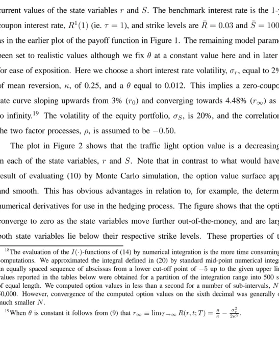
(15) 3 Numerical illustrations As indicated above, formula (14) of Proposition 1 is easily evaluated. For the various numerical illustrations below we coded the formula in Visual Basic for Excel, using Microsoft Excel’s built-in standard functions wherever possible (such as the one for the standard normal distribution function). Although Visual Basic is notoriously slow compared to standard alternatives such as C++ and Delphi Pascal, our program executed and delivered prices virtually instantly.18 Figure 2 shows a plot of traffic light option values with 1 year to maturity for different current values of the state variables r and S. The benchmark interest rate is the 1-year zero¹ = 0:03 and S¹ = 100 precisely coupon interest rate, R1 (1) (ie. ¿ = 1), and strike levels are R as in the earlier plot of the payoff function in Figure 1. The remaining model parameters have been set to realistic values although we fix μ at a constant value here and in later examples for ease of exposition. Here we choose a short interest rate volatility, ¾r , equal to 2%, a speed of mean reversion, ·, of 0.25, and a μ equal to 0.012. This implies a zero-coupon interest rate curve sloping upwards from 3% (r0 ) and converging towards 4.48% (r1 ) as time goes to infinity.19 The volatility of the equity portfolio, ¾S , is 20%, and the correlation between the two factor processes, ½, is assumed to be ¡0:50. The plot in Figure 2 shows that the traffic light option value is a decreasing function in each of the state variables, r and S. Note that in contrast to what would have been the result of evaluating (10) by Monte Carlo simulation, the option value surface appears nice and smooth. This has obvious advantages in relation to, for example, the determination of numerical derivatives for use in the hedging process. The figure shows that the option values converge to zero as the state variables move further out-of-the-money, and are largest when both state variables lie below their respective strike levels. These properties of the option 18 The evaluation of the I(¢)-functions of (14) by numerical integration is the more time consuming part of the computations. We approximated the integral defined in (20) by standard mid-point numerical integration using an equally spaced sequence of abscissas from a lower cut-off point of ¡5 up to the given upper limit. Option values reported in the tables below were obtained for a partition of the integration range into 500 sub-intervals of equal length. We computed option values in less than a second for a number of sub-intervals, N , as high as 50,000. However, convergence of the computed option values on the sixth decimal was generally obtained for much smaller N . 19. When μ is constant it follows from (9) that r1 ´ limT !1 R(r; t; T ) =. 13. μ ·. ¡. 2 ¾r . 2·2.

(16) Traffic light option value κ=0.25, θ=0.012,σ r =0.02, σ S =0.20, ρ=−0.50, Τ=τ=1. S = 100 , R = 0.03. 0.5. 0.4 0.35 0.3 0.25 0.2 0.00% 1.00% 2.00%. 0.15 0.1 0.05. 3.00%. 0. 115. 105. 110. 95. 5.00%. 100. 85. 90. 75. 80. 65. 70. 4.00%. Interest rate, r. Option value, V(R,S,T). 0.45. Equity portfolio value, S. Figure 2: Traffic light option values for different current values of the state variables, r and S. value function are completely as expected for a multiplicative put option such as the traffic light option. For the same set of interest rate process parameters and equity value process parameters as in Figure 2, Table 1 illustrates the dependence of traffic light option values on the correlation parameter, ½, time to maturity of the option, T , and on time to maturity, ¿ , of the underlying zero-coupon interest rate, R¿ (¢).20 The table confirms that ½ is indeed a key parameter. When correlation is strongly negative, the options are seen to be almost worthless, and option values increase sharply as ½ increases. These effects are of course closely related to the fact that the table considers (near) at-the-money (ATM) options for which the state variables must move in the same direction and drop below their respective strike levels in order for a payoff to obtain.. 20. Note that option values in Tables 1 and 2 are multiplied by 100 due to their small absolute values.. 14.

(17) Table 1:. ¿ =0. ¿ =1. ¿ =5. Traffic Light Option values £100 Dependence on correlation, time to maturity, and ”length” of benchmark interest rate. ½ -0.99 -0.75 -0.50 -0.25 0.00 0.25 0.50 0.75 0.99 -0.99 -0.75 -0.50 -0.25 0.00 0.25 0.50 0.75 0.99 -0.99 -0.75 -0.50 -0.25 0.00 0.25 0.50 0.75 0.99. 0.25 0.000 0.125 0.397 0.770 1.232 1.780 2.414 3.147 3.980 0.000 0.056 0.219 0.466 0.788 1.181 1.646 2.191 2.810 0.000 0.001 0.010 0.035 0.080 0.142 0.222 0.316 0.410. · = 0:25; μ = 0:012; ¾r = 0:02; ¾S = 0:20 ¹ = r0 = 0:03; S¹ = S(0) = 100 R T (years) 0.50 1 2 3 5 10 0.000 0.000 0.000 0.000 0.000 0.002 0.208 0.315 0.417 0.453 0.456 0.398 0.687 1.109 1.601 1.840 1.973 1.734 1.357 2.242 3.338 3.917 4.305 3.832 2.190 3.660 5.527 6.544 7.257 6.475 3.178 5.342 8.120 9.643 10.708 9.500 4.324 7.290 11.100 13.177 14.578 12.789 5.646 9.530 14.492 17.149 18.829 16.252 7.148 12.054 18.240 21.451 23.271 19.678 0.000 0.000 0.000 0.000 0.000 0.001 0.111 0.191 0.274 0.307 0.317 0.284 0.432 0.759 1.156 1.356 1.478 1.312 0.911 1.612 2.506 2.988 3.321 2.971 1.530 2.709 4.242 5.088 5.692 5.088 2.280 4.032 6.322 7.589 8.483 7.525 3.162 5.578 8.729 10.456 11.625 10.179 4.190 7.367 11.475 13.682 15.075 12.972 5.354 9.373 14.490 17.152 18.656 15.721 0.000 0.000 0.000 0.000 0.000 0.000 0.005 0.018 0.041 0.054 0.065 0.066 0.045 0.134 0.277 0.362 0.429 0.401 0.137 0.365 0.724 0.939 1.110 1.019 0.280 0.706 1.358 1.748 2.051 1.854 0.472 1.148 2.159 2.753 3.197 2.841 0.711 1.685 3.108 3.926 4.500 3.922 0.990 2.307 4.188 5.236 5.915 5.045 1.279 2.955 5.300 6.565 7.311 6.116. 20 0.007 0.268 1.091 2.400 4.047 5.905 7.874 9.881 11.793 0.005 0.196 0.830 1.862 3.173 4.658 6.235 7.841 9.367 0.001 0.050 0.261 0.640 1.144 1.728 2.350 2.980 3.569. In the horizontal dimension Table 1 indicates that for the present choice of parameters option values tend to peak for a time to maturity between 3 and 10 years. In fact, traffic light option values will in general peak and then converge towards 0 as T ! 1 independently of the current value of the state variables. These properties are not surprising in light of the fact 15.

(18) that both the straight European interest rate floorlet, and the plain vanilla European equity put – when considered separately – are known to possess similar properties given the assumptions about market dynamics applied here. The time to maturity – or ”length” – of the zero-coupon interest rate underlying the traffic light option contract is varied in the three panels of Table 1. The first panel contains traffic light option values for the case where the instantaneous short rate is the benchmark interest rate (ie. when ¿ = 0), and the second and third panels consider options on 1-year and on 5-year zero-coupon interest rates, respectively. It is observed that option values are smaller when ¿ is larger. There are two explanations for this. Firstly, longer interest rates are simply less volatile than shorter rates, both in this model (follows from (9)) and in practice, and lower volatility of the underlying generally implies lower option values. Secondly, since our parameter choice realisticly implies a slightly upward sloping term structure curve, put options on longer rates will entail smaller intrinsic option values, ceteris paribus. Table 2 provides representative values of in-the-money (ITM), at-the-money, as well as out-of-the-money (OTM) traffic light options for a more varied span of parameter values. Throughout this table the benchmark interest rate is the instantaneous short rate. The option values behave as expected: They increase with the correlation, and they increase in both partial measures of volatility, ¾S and ¾r . Of course, ITM options are more valuable than ATM options, which are in turn more valuable than OTM options. The qualitative effects are unaffected by the choice of the ”length” of the underlying interest rate.. 16.

(19) Table 2: Traffic Light Option values £100 · = 0:25; μ = 0:012 ¹ = 0:03; S¹ = 100; T = 1; ¿ = 0 R. ½. ¾S 0:10. ¡0:50. 0:20. 0:30. ½. ¾S 0:10. 0:00. 0:20. 0:30. ½. ¾S 0:10. 0:50. 0:20. 0:30. S0 95 100 105 95 100 105 95 100 105. S0 95 100 105 95 100 105 95 100 105. S0 95 100 105 95 100 105 95 100 105. ¾r = 0:01 r0 0.025 0.030 0.035 0.778 0.317 0.108 0.314 0.118 0.037 0.107 0.037 0.010 1.284 0.532 0.185 0.827 0.330 0.110 0.517 0.198 0.063 1.849 0.775 0.274 1.392 0.570 0.196 1.039 0.415 0.139 ¾r = 0:01 r0 0.025 0.030 0.035 1.894 0.991 0.458 1.031 0.535 0.245 0.499 0.256 0.116 3.205 1.705 0.802 2.389 1.268 0.595 1.743 0.923 0.432 4.529 2.425 1.147 3.752 2.006 0.948 3.088 1.649 0.779 ¾r = 0:01 r0 0.025 0.030 0.035 3.283 1.918 0.997 2.063 1.231 0.657 1.161 0.709 0.389 5.628 3.334 1.755 4.507 2.706 1.446 3.533 2.150 1.167 7.862 4.665 2.455 6.833 4.092 2.176 5.896 3.564 1.916. 17. ¾r = 0:02 r0 0.025 0.030 1.696 1.080 0.695 0.422 0.240 0.139 2.697 1.750 1.743 1.109 1.093 0.682 3.836 2.514 2.892 1.872 2.162 1.382 ¾r = 0:02 r0 0.025 0.030 4.064 2.932 2.252 1.610 1.112 0.786 6.685 4.900 5.004 3.660 3.667 2.675 9.348 6.894 7.758 5.715 6.396 4.707 ¾r = 0:02 r0 0.025 0.030 6.947 5.303 4.444 3.411 2.560 1.975 11.652 9.017 9.372 7.290 7.383 5.773 16.142 12.534 14.056 10.957 12.153 9.512. 0.035 0.658 0.245 0.077 1.089 0.676 0.407 1.581 1.162 0.847. 0.025 2.763 1.150 0.404 4.230 2.743 1.726 5.937 4.483 3.356. 0.035 2.054 1.117 0.540 3.490 2.600 1.896 4.938 4.090 3.365. 0.025 6.511 3.673 1.851 10.413 7.828 5.762 14.410 11.981 9.897. 0.035 3.943 2.554 1.489 6.793 5.524 4.400 9.471 8.315 7.250. 0.025 10.972 7.142 4.211 18.024 14.562 11.530 24.769 21.610 18.723. ¾r = 0:03 r0 0.030 2.024 0.814 0.275 3.158 2.019 1.253 4.473 3.349 2.485 ¾r = 0:03 r0 0.030 5.194 2.904 1.448 8.437 6.328 4.646 11.744 9.754 8.049 ¾r = 0:03 r0 0.030 9.102 5.929 3.495 15.149 12.271 9.741 20.900 18.275 15.870. 0.035 1.453 0.564 0.184 2.314 1.458 0.891 3.309 2.455 1.806. 0.035 4.091 2.266 1.119 6.750 5.051 3.699 9.451 7.842 6.464. 0.035 7.468 4.871 2.874 12.590 10.227 8.141 17.432 15.280 13.300.

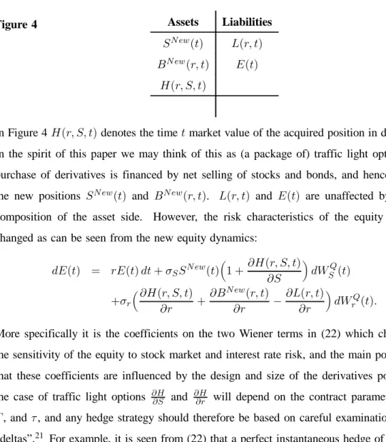
(20) 4 The traffic light option as a hedging instrument In this section the potential usefulness of the traffic light option as a hedge instrument for the balance sheet of a typical pension fund or life insurance company will be further investigated. We do this first from a theoretical point of view, and then by way of an illustrative numerical example inspired by the theoretical results. The theoretical analysis will take the following simplified time t balance sheet as its point of departure:. Figure 3. Assets. Liabilities. S(t). L(r; t). B(r; t). E(t). Reflecting the main entries of a typical L&P company, the asset side of the balance sheet consists of the market value of stocks, S(t), and bond investments, B(r; t). On the liability side L(r; t) denotes the market value of the company’s fixed pension obligations. The notation underlines that the bond value and the market value of the ”bond like” promised pension benefits depend on the interest rate. E(t) is the market value of the equity at time t. This is determined residually as S + B ¡ L in order to ensure a balanced sheet. The balance sheet in Figure 3 is unmatched in the sense that equity is exposed to both interest rate and stock market risk. Formally, assuming our previous model holds and using Ito’s lemma on the above expression for the equity, we can infer the following about the equity’s Q-dynamics dE(r; S; t) =. r(t)E(t) dt + ¾S S(t) dWSQ (t) + ¾r. μ. @B(r; t) @L(r; t) ¡ @r @r. ¶. dWrQ (t): (21). This relation emphasizes that equity is risky to the extent that the company invests in the stock market (ie. when S(t) 6 = 0), and to the extent that the ”duration” of liabilities and bond investments differ (ie. when. @B @r. 6@L = @r ). In theory this asset liability mismatch can be easily. repaired by selling all stocks and investing in bonds such that. @B @r. =. @L @r .. For various reasons,. however, this is rarely done in practice. One practical problem preventing such a strategy is that pension liabilities typically are very ”long” obligations with durations of 20 years or more. Investment grade bonds with similar durations are often in very limited supply. In 18.

(21) addition, the earlier discussed focus of the typical L&P portfolio manager on capturing the equity premium undoubtedly hampers the simple perfect matching strategy. Hence, what is more often done in practice is that companies attempt to control the risk to the equity (and thus ultimately to policyholders’ savings) via a rearrangement of the asset side to include appropriately structured derivatives. Following such a rebalancing exercise, the time t balance sheet would look as follows: Assets. Liabilities. S N ew (t). L(r; t). B N ew (r; t). E(t). Figure 4. H(r; S; t). In Figure 4 H(r; S; t) denotes the time t market value of the acquired position in derivatives. In the spirit of this paper we may think of this as (a package of) traffic light options. The purchase of derivatives is financed by net selling of stocks and bonds, and hence we have the new positions S N ew (t) and B N ew (r; t). L(r; t) and E(t) are unaffected by the new composition of the asset side. However, the risk characteristics of the equity will have changed as can be seen from the new equity dynamics: ³ @H(r; S; t) ´ dE(t) = rE(t) dt + ¾S S N ew (t) 1 + dWSQ (t) @S ³ @H(r; S; t) @B N ew (r; t) @L(r; t) ´ + ¡ dWrQ (t): +¾r @r @r @r. (22). More specifically it is the coefficients on the two Wiener terms in (22) which characterize the sensitivity of the equity to stock market and interest rate risk, and the main point here is that these coefficients are influenced by the design and size of the derivatives position. In the case of traffic light options. @H @S. and. @H @r. ¹ S, ¹ will depend on the contract parameters R,. T , and ¿ , and any hedge strategy should therefore be based on careful examination of these ”deltas”.21 For example, it is seen from (22) that a perfect instantaneous hedge of the equity 21 Although we do not have traffic light option deltas in closed form, accurate numerical first derivatives are easily obtained using the closed valuation formula of Proposition 1.. 19.

(22) can be obtained by designing a traffic light option position which satisfies @H(r; S; t) @S @H(r; S; t) @r. = ¡1. @L(r; t) @B N ew (r; t) ¡ @r ³ @r ´ ³ ´ N ew H(r; S; t) = S(t) ¡ S (t) + B(r; t) ¡ B N ew (r; t) : =. While it may be the strategic decision of pension fund managers to hedge away all equity risk in this way at certain times, it is unlikely to be their typical investment objective as also argued earlier. Although it is difficult to make statements about L&P portfolio managers’ investment objectives in general, they undoubtedly involve some form of optimization of expected returns and the proportion of funds invested in stocks, subject to risk measures similar to the diffusion coefficients in (22), ruin probabilities, and regulatory constraints like the traffic light stress tests described earlier. The remainder of this section presents a numerical example created with the purpose of illustrating how an L&P company may use traffic light options for a ’regulatory hedge’ in the sense that the options are designed specifically to make the company ’look good’ in the worst of the traffic light scenarios (the yellow scenario) and such that operation under green light is ensured. Needless to say a proper ’economic hedge’ may involve additional considerations into which we shall not dwell further here. The point of departure of the example is a representative balance sheet with a simple and typical unmatched (or mismatched) distribution of assets and liabilities, cf. the theoretical considerations above. We focus on the solvency percentage (or solvency ratio) of this balance sheet – defined as free equity divided by the market value of liabilities,. E L. – and study the sensitivity of this. quantity to changes in the state variables. The sensitivity analysis is carried out for both a simple, unhedged balance sheet, and for a balance sheet that has been hedged with a number of appropriately designed traffic light options. The illustration starts out at time 0 from a normalized balance sheet as illustrated in Figure 5 below. The asset side is comprised of 30 (units of account) invested in a well-diversified stock portfolio and 70 units invested in bonds. Apart from the fact that pension funds typically have a minor part (2-8%) of their funds invested in real estate, this is a realistic asset. 20.

(23) allocation.22. Figure 5 Assets. Liabilities. Stocks. 30.00. 92.00. Bonds (D = 6 years). 70.00. 8.00. 100.00. 100.00. Total. Pension obligations (D = 20 years) Equity (Solvency ratio: 8.70%) Total. The bond investment is further assumed to be characterized by a duration of 6 years. Again this is inspired by actual pension fund portfolio compositions. In practice pension funds often face a limited market supply of investment grade bonds with durations higher than 6-8 years, and “long” bond portfolios can therefore be difficult to acquire. On the liability side the market value of the “bond like” pension obligations is set to 92 units of account and an equal percentage of the balance sheet sum. These are very long obligations with an assumed duration of 20 years. This is not unrealistic. Actual pension fund liability durations typically vary between 15 and 25 years depending on the exact age distribution of the policy holders. In the present example the initial free equity is thus 8 units of account, and the solvency ratio thus equals. 8 92. or 8.70%.. Now, in order to perform the desired sensitivity analysis we assume that the market values and dynamics of the balance sheet entries, ie. the stock portfolio, the bond investment, and the liabilities, are in accordance with the model given in (3)–(5). In particular we assume that the interest rate parameters are given as r0 = 0:04, · = 0:25, μ = 0:012, and ¾r = 0:02. For simplicity the bond investment and the liability entries are assumed to be zero-coupon bonds with maturities (=durations) equal to 6 and 20 years respectively. The present values of 70 and 92 imply initial bond and pension liability “notionals” of 90.58 and 222.52, respectively. We can now study changes in the entries of this unhedged or “naked” balance sheet – and thus also in the solvency ratio – as a consequence of changes in the state variables, the short interest rate and the value of the stock portfolio. For a first illustration suppose that the short rate drops from 4% to 3%, and that the stock portfolio loses 30% of its value 22 Before the DFSA’s introduction of the traffic light stress test system, the maximum allowable equity portfolio weight in stocks was a fixed percentage. It was 40% up to 1997, and following extensive pressure on regulators from pension fund managers, it was raised to 50% between 1997 and 2000, cf. the discussion in the introduction.. 21.

(24) right after time 0.23 As a consequence of these changes in the state variables the value of the bond portfolio will increase to 72.21, but liabilities increase to 95.73. The equity portfolio value drops to 21, and the resulting market value based balance sheet now looks as follows.. Figure 6 Liabilities. Assets Stocks. 21.00. 95.73. Pension obligations (D = 20 years). Bonds (D = 6 years). 72.21. -2.52. Equity (Solvency ratio: -2.63%). Total. 93.21. 93.21. Total. As can be seen from Figure 6 the solvency percentage has dropped by more than 11 percentage points, and the ”company” is now technically insolvent. A more complete picture of the solvency ratio’s response to changes in the state variables can be seen in Figure 7 below.. Figure 7. The Unhedged Balance Sheet Solvency Percentage when interest rates and equity values change. Solvency Percentage. 22.50%. 13.50%-22.50% 4.50%-13.50%. 13.50%. -4.50%-4.50%. 4.50% 20% 10% 0% -10% Percentage change in -20% equity portfolio value -30%. 3.00%. 2.00%. 1.00%. 0.00%. -1.00%. -2.00%. -3.00%. -4.50%. Percentage point change in short interest rate. Figure 7: Sensitivity of solvency ratio to changes in the state variables in the unhedged balance sheet. r0 = 0:04, · = 0:25, μ = 0:012, and ¾r = 0:02. 23. The size of the shocks to the state variables is inspired by the DFSA’s yellow light scenario. Note, however, that stricto sensu our dynamic model is not consistent with discontinuous jumps in the state variables. Moreover, in the Hull-White/Vasicek model term structure movements are not parallel and long rates will always change less than the short rate.. 22.

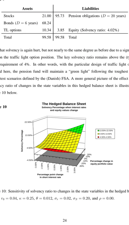
(25) The plot in Figure 7 clearly shows how the unhedged pension fund is exposed to the risk of interest rate and stock price shocks. Without protection the solvency ratio will decrease in an almost linear fashion when the interest rate or equity values fall, and most dramatically so when both state variables fall. Now, the traffic light option was of course created with the purpose of providing a hedge instrument for precisely these simultaneous adverse changes in the stock prices and in the interest rate. Let us therefore illustrate how – with appropriate traffic light options added – the solvency percentage will respond less dramatically to changes in S0 and in r0 . For this purpose we must specify numerical values for the stock portfolio volatility, ¾S , and the correlation coefficient, ½, in order to be able to value the traffic light option. Suppose therefore that ¾S = 0:20 and that ½ = 0:0. Finally, suppose that 225 traffic light options with ¹ = 0:04, S¹ = 30, and T = 5 are acquired. The benchmark interest rate is the 3-year zeroR coupon rate, ie. ¿ = 3. This option package design was inspired in part by a consideration of the diffusion coefficients of (22) corresponding to the present example. Our model prices the traffic light options at 0.01711 a piece. For simplicity the total value of 3.85 for the 225 options will be financed by selling bonds. While the liability side of the balance sheet is unaffected by this disposition, the asset side of the new balance sheet will contain a new entry and will take the following form: Figure 8 Liabilities. Assets Stocks. 30.00. Bonds (D = 6 years). 66.15. TL options Total. 92.00. 3.85. 8.00. 100.00. 100.00. Pension obligations (D = 20 years). Equity (Solvency ratio: 8.70%) Total. Of course, the initial solvency ratio is unaffected by the purchase of options and is again 8.70%. We will now study the response of the solvency ratio of this hedged balance sheet to changes in the state variables. Consider first the (yellow light) scenario where r0 drops from 4% to 3%, and where stocks lose 30% of their value. Following this scenario the balance sheet will look as follows: 23.

(26) Figure 9 Assets. Liabilities. Stocks. 21.00. 95.73. Bonds (D = 6 years). 68.24. TL options. 10.34. 3.85. Total. 99.58. 99.58. Pension obligations (D = 20 years). Equity (Solvency ratio: 4.02%) Total. Note that solvency is again hurt, but not nearly to the same degree as before due to a significant gain on the traffic light option position. The key solvency ratio remains above the (typical) FSA requirement of 4%. In other words, with the particular design of traffic light options applied here, the pension fund will maintain a “green light” following the toughest of the stress test scenarios defined by the (Danish) FSA. A more general picture of the effect on the solvency ratio of changes in the state variables in this hedged balance sheet is illustrated in Figure 10 below. The Hedged Balance Sheet. Figure 10. Solvency Percentage when interest rates and equity values change. Solvency Percentage. 22.50%. 13.50%-22.50% 4.50%-13.50%. 13.50%. -4.50%-4.50%. 4.50%. 20% 10% 0% -10% Percentage change in -20% equity portfolio value -30% 3.00%. 2.00%. 1.00%. 0.00%. -1.00%. -2.00%. -3.00%. -4.50%. Percentage point change in short interest rate. Figure 10: Sensitivity of solvency ratio to changes in the state variables in the hedged balance sheet. r0 = 0:04, · = 0:25, μ = 0:012, ¾r = 0:02, ¾S = 0:20, and ½ = 0:00.. 24.

(27) As is clear from a comparison of this plot with Figure 7, the effect of adding the traffic light options has been to “twist” the solvency percentage surface upwards in the area of critically low state variables. There are now no states with solvency ratios below 3%. The price for this protection is of course paid by sacrificing part of the “upside” in the sense that in the presence of traffic light option coverage, solvency will increase less in response to favorable changes in the state variables in comparison with the unhedged balance sheet situation.. 5 Conclusions This paper has introduced, priced, and analyzed a new instrument in the landscape of exotic financial derivatives – the traffic light option. Traffic light options have been developed and introduced recently by a number of investment banks in order to suit the needs of Danish L&P companies, which must comply with the Danish FSA’s traffic light stress tests introduced in mid-2001. This scenario-based risk supervision system basically tests whether the base capital of L&P companies can withstand certain pre-defined shocks to interest rates and stock prices – the traffic light scenarios. L&P company solvency suffers when interest rates or stock prices fall, and they are in double jeopardy when such falls occur simultaneously as in the DFSA’s red and yellow light scenarios. Traffic light options are thus designed to pay off and provide solvency protection for L&P companies in scenarios where both interest rates and stock prices fall. In this paper we have introduced a continuous time dynamic framework in which the traffic light option can be analyzed using standard assumptions of perfect markets and absence of arbitrage. The main contribution of this paper was a closed form solution for the value of the traffic light option. The implementation of the formula was discussed and numerical examples were provided to illustrate the usefulness of the traffic light option for hedging the typical L&P company balance sheet. There is no doubt that traffic light options hold great potential as hedging instruments not only for Danish L&P companies but also on a world-wide scale since regulatory authorities in more and more countries implement market value based financial reporting standards and. 25.

(28) solvency tests. However, one possible obstacle for the success of traffic light options concerns the estimation of the correlation coefficient of the model. As the numerical section has shown, the correlation between equity and interest rate risk is an enormously important determinant for the value of traffic light options. It is a parameter which is difficult to estimate accurately, and it may in fact not be constant even over short time intervals. One might therefore worry that the uncertainty surrounding the true value of this parameter may lead sellers of traffic light options (investment banks) to set premiums on the “safe side”. Traffic light options may thus in turn appear “expensive” to potential buyers, who may therefore decide to stick with the imperfect strategy of hedging interest rate and stock market risk separately. Modelling time-varying correlation and establishing corresponding traffic light option pricing formulas is thus one obvious extension of our work. Another interesting subject for future research would be a more normative investigation into which types of derivative instruments – if any – that would in fact be best suited for managing the risks of typical L&P company balance sheets. This would necessarily involve the non-trivial task of defining both some metric for measuring optimality and an appropriate way of quantifying regulatory and other restrictions facing L&P companies. The traffic light option analyzed in this paper is just one of many candidates in such a horse-race, and it is unlikely to become the final exotic derivative instrument proposed for risk management of financial institutions.. 26.

(29) Appendix. A Proof of Proposition 1 The explicit solutions for time T > t of the SDEs in (11) and (12) can be written as (see e.g. Arnold (1992)) ¡·(T ¡t). r(T ) = r(t)e Z +¾r. +. Z. T. t. e·(u¡T ) μ(u) du ¡. T. ¾r2 2 ª (T ¡ t) 2. T. e·(u¡T ) dWrQ (u); t Z T ln S(T ) = ln S(t) + μ(u)ª(T ¡ u) du t · 2 ¸ 1 2 ¾r ½¾r ¾S + ¾S (T ¡ t) ¡ 2+ · · 2 · 2 ¸ ¾r ½¾r ¾S + 2+ + r(t) ª(T ¡ t) · · · 2¸ ¾ + r ª2 (T ¡ t) 2· Z T Z T T T dWSQ (u) + ¾r ª(T ¡ u) dWrQ (u): +¾S t. (A.1). (A.2). t. From (A.1), (A.2), and (9) it follows that the joint conditional QT -distribution of R¿ (T ) and ln S(T ) is bivariate normal (see e.g. Kotz, Balakrishnan, and Johnson (2000)): 0 1 ³ mR ´ ³ v 2 ¾RS ´ R A; N@ ; mS ¾RS vS2 2 , v 2 , and ¾ with parameter functions mR , mS , vR RS as given in (15)-(19). The coefficient S. of correlation is given as ½RS =. ¾RS : vR vS. Now, the fundamental QT -expectation of the payoff function in (10) can be decomposed as ª © ª © ¹¢E S¢1 ¹ ¢1 ¹ ¹ ¢ S¹ ¢ E 1 ¹ ¢ 1 ¹ ¡ R R R<R S<S R<R S<S © ª © ª ¡S¹ ¢ E R ¢ 1R<R¹ ¢ 1S<S¹ + E R ¢ S ¢ 1R<R¹ ¢ 1S<S¹ ; 27. (A.3).

(30) with obvious shorthand notation. Next, tedious integration over the bivariate normal density for (R; ln S) for each of the expectation terms in (A.3) in turn yields ¶ μ¹ ª © R ¡ mR ln S¹ ¡ mS ; ; ½RS = M E 1R<R¹ ¢ 1S<S¹ vR vS ¶ μ¹ © ª R ¡ mR ¡ ¾RS ln S¹ ¡ mS ¡ vS2 2 mS + 12 vS E S ¢ 1R<R¹ ¢ 1S<S¹ ¢M ; ; ½RS = e vR vS μ¹ ¶ © ª R ¡ mR ln S¹ ¡ mS E R ¢ 1R<R¹ ¢ 1S<S¹ ; ; ½RS = mR M vR vS 8 9 0 1 ¹ ln S¡m S < = ¡ ½ " ~ RS vS @ A q ¹ +vR E "~ ¢ N ¢ 1 R¡mR "~< v : ; R 1 ¡ ½2 RS. ¶ μ¹ ª © 1 2 R ¡ mR ¡ ¾RS ln S¹ ¡ mS ¡ vS2 ; ; ½RS = (mR + ¾RS )emS + 2 vS ¢ M E R ¢ S ¢ 1R<R¹ ¢ 1S<S¹ vR vS 9 8 1 0 ¹ ln S¡m S = < ¡ v ¡ ½ " ~ S RS 2 vS mS + 12 vS A @ q ¹ ¢ 1 R¡mR ¢ E "~ ¢ N +vR e ; "~< v ¡½RS vS ; : R 1 ¡ ½2RS where M (¢; ¢; ») denotes the cumulative probability in the standardized bivariate normal distribution with correlation coefficient », and where "~ » N (0; 1). Finally, collection of terms yields the desired result. 2. 28.

(31) References Agca, S. and D. M. Chance (2003): “Speed and Accuracy Comparison of Bivariate Normal Distribution Approximations for Option Pricing,” Journal of Computational Finance, 6(4):61–96. Arnold, L. (1992): Stochastic Differential Equations: Theory and Applications, Krieger Publishing Company, Malabar, Florida. Black, F. and M. Scholes (1973):. “The Pricing of Options and Corporate Liabilities,”. Journal of Political Economy, 81(3):637–654. Boyle, P. P. (1977): “Options: A Monte Carlo Approach,” Journal of Financial Economics, 4:323–338. Brigo, D. and F. Mercurio (2006): Interest Rate Models – Theory and Practice: With Smile, Inflation and Credit, Springer-Verlag, Berlin, Germany. Briys, E. and F. de Varenne (1997): “On the Risk of Life Insurance Liabilities: Debunking Some Common Pitfalls,” Journal of Risk and Insurance, 64(4):673–694. DFSA (2005): “Traffic light stress test system in Denmark has served the industry well,” Global Pensions, (April):11. Drezner, Z. (1978):. “Computation of the Bivariate Normal Integral,” Mathematics of. Computation, 32(1):277–279. Haug, E. G. (1997): The Complete Guide to Option Pricing Formulas, McGraw-Hill, New York. Hull, J. and A. White (1990): “Pricing Interest Rate Derivative Securities,” The Review of Financial Studies, 3(4):573–592. (1994): “Numerical Procedures for Implementing Term Structure Models I: Single-Factor Models,” Journal of Derivatives, Fall:7–16. Hull, J. C. (2003): Options, Futures, and other Derivatives, Prentice-Hall, Inc., 5th edition. 29.

(32) (2006):. Options, Futures, and other Derivatives, Prentice-Hall, Inc., 6th. edition. Jørgensen, P. L. (2004): “On Accounting Standards and Fair Valuation of Life Insurance and Pension Liabilities,” Scandinavian Actuarial Journal, 104(5):372–394. Kotz, S., N. Balakrishnan, and N. L. Johnson (2000): Continuous Multivariate Distributions: Vol. 1: Models and Applications, John Wiley & Sons, Inc., New York. Longstaff, F. A. and E. S. Schwartz (1995): “A Simple Approach to Valuing Risky Fixed and Floating Rate Debt,” The Journal of Finance, L(3):789–819. Menon, R. (2005): “Sweden set to introduce ‘traffic light’ stress tests,” Global Pensions, (March):1. Mercer Oliver Wyman (2004): “Life at the End of the Tunnel: The Capital Crisis in the European Life Sector,” Mercer Oliver Wyman Research Report. Shimko, D. C., N. Tejima, and D. R. van Deventer (1993): “The Pricing of Risky Debt when Interest Rates are Stochastic,” The Journal of Fixed Income, pages 58–65. Sørensen, C. (1999): “Dynamic Asset Allocation and Fixed Income Management,” Journal of Financial and Quantitative Analysis, 34(4):513–532. The Economist (2004a): “A Bad Business,” (February 14th):75. (2004b): “Deeper into the Red,” (February 7th):71–72. Vasicek, O. (1977): “An Equilibrium Characterization of the Term Structure,” Journal of Financial Economics, 5:177–188. Watson-Wyatt (2003): “Pensions in Crisis,” Insider, 13(9):1–15. Wilmott, P. (1998): Derivatives: The Theory and Practice of Financial Engineering, John Wiley & Sons.. 30.

(33) Working Papers from Finance Research Group. F-2006-08. Peter Løchte Jørgensen: Traffic Light Options.. F-2006-07. David C. Porter, Carsten Tanggaard, Daniel G. Weaver & Wei Yu: Dispersed Trading and the Prevention of Market Failure: The Case of the Copenhagen Stock Exhange.. F-2006-06. Amber Anand, Carsten Tanggaard & Daniel G. Weaver: Paying for Market Quality.. F-2006-05. Anne-Sofie Reng Rasmussen: How well do financial and macroeconomic variables predict stock returns: Time-series and cross-sectional evidence.. F-2006-04. Anne-Sofie Reng Rasmussen: Improving the asset pricing ability of the Consumption-Capital Asset Pricing Model.. F-2006-03. Jan Bartholdy, Dennis Olson & Paula Peare: Conducting event studies on a small stock exchange.. F-2006-02. Jan Bartholdy & Cesário Mateus: Debt and Taxes: Evidence from bankfinanced unlisted firms.. F-2006-01. Esben P. Høg & Per H. Frederiksen: The Fractional Ornstein-Uhlenbeck Process: Term Structure Theory and Application.. F-2005-05. Charlotte Christiansen & Angelo Ranaldo: Realized bond-stock correlation: macroeconomic announcement effects.. F-2005-04. Søren Willemann: GSE funding advantages and mortgagor benefits: Answers from asset pricing.. F-2005-03. Charlotte Christiansen: Level-ARCH short rate models with regime switching: Bivariate modeling of US and European short rates.. F-2005-02. Charlotte Christiansen, Juanna Schröter Joensen and Jesper Rangvid: Do more economists hold stocks?. F-2005-01. Michael Christensen: Danish mutual fund performance - selectivity, market timing and persistence.. F-2004-01. Charlotte Christiansen: Decomposing European bond and equity volatility..

(34) ISBN 87-7882-178-9. Department of Business Studies. Aarhus School of Business Fuglesangs Allé 4 DK-8210 Aarhus V - Denmark Tel. +45 89 48 66 88 Fax +45 86 15 01 88 www.asb.dk.

(35)

No results found