Measuring Risk Aversion From Excess Returns on a Stock Index

NBER WORKING PAPER SERIES

NEASURING RISK AVERSION FROW EXCESS RETURNS ON

A

STOCK INDEX

Ray Chou Robert F. Engle

Alex Kane

Working Paper No. 3643

NATIONAL BUREAU OF ECONONIC RESEARCH 1050 Nassaohusetts Avenue

Cambridge, MA 02138 Noroh 1991

he would like to thank Stephen Brown, Angelo Nelino, Michael Rothschild, Ross Starr, Larry Wall, and an anonymous referee far helpful oormsents. We are also grateful to participants at various conferences and seminars where this paper was presented, inoludinp the NBER, WFA, UCSD, UC Santa Barbara, Georgia Tech, and Emory University. This paper is part of the NBER's research program in Financial Narkets and Monetary Economics. Any

opinions expressed are those of the authors and not those of the Notional Bureau of Economic Research.

MEASURING RISK AVERSION FROM EXCESS RETURNS ON A STOCK INDEX ABSTRACT

We distinguish the measure of risk aversion from the slope coefficient in the linear relationship between the mean excess return on a stock index and its variance. Even when risk

aversion is constant, the latter can vanj significantly with the relative share of stocks in the risky wealth portfolio, and with the beta of unobserved wealth on stocks.

We introduce a statistical model with ARCH disturbances and a time-varying parameter in the mean (TVP ARCH-N). The model decomposes the predictable component in stock returns into two parts: the time-varying price of volatility and the time-varying volatility of returns. The relative share of stocks and the beta of

the

excluded components of wealth on stocks are instrumented by

macroeconomic

variables.

The ratio of corporate profit over national income and the inflation rate ore found to be important forces in the dynamics of stock price volatility.

Ray Chou Robert F. Engle

Ivan Allen College of Management, Department of Economics Policy and International Affairs University of California, Georgia Institute of Technology San Diego

225 North Avenue, NW La Jolla, CA 92093-0508 Atlanta, GA 30332

Alex Kane

Graduate School of Internaticnal Relations and Pacific Studies

University of California, San Diego La

Jolla,

CA

92093-0519

MEASURING RISK AVERSION FROM EXCESS RETURNS ON A STOCK INDEX

I. Introduction

The trade—off between risk and return is central to the theory of finance. The Capital Asset Pricing Model (CAPM( of Sharpe (1964), Lintner (1965) , and Mossin (1966) was first to provide a comprehensive

framework for detennining asset prices with the theme that only systematic risk is rewarded by the market. The risk premium on the market portfolio was linked to investor risk aversion by Totin (1958)

and Pratt (1964)

Morton (1969, 1973) shows that a lifetime consumption—investment model yields risk premia of the same form as the single period model when the _{investment opportunity set is constant and portfolios} are continuously rebalanoed. This result will still hold when the variance of the market portfolio varies randomly and cannot be hedged.

Bodie, Kane, and McDonald (1953) and Pindyck (1985) assume a single factor CAPM, and use a 'reasonable" parameter for relative risk aversion

(between 3 and 4), as defined in Pratt (1964), in an attempt to infer risk _{premiums from estimated variances.} Inferring in the opposite direction Friend and Blume (1975) attempt to estimate the coefficient of

relative risk aversion of a representative investor using estimates of relative portfolio shares of financial assets, and the ax-post excess return average and variance of these assets. While tney pot the estimate of relative risk aversion at about 2, their method uses the unconditional variance, which is not consistent with the model

assumption of portfolio rebalancing. There, the _{risk premium ougho to}

be determined _{by the conditional or expected} vsrience.

GARCH-M models of stock returns (see Bollerslev, Chou, and Kroner (5CR, 1990)) for an extensive review and references _{of ARCH modeling in} finance) jointly estimate the _{time varying conditional} variance and a

constant mean-variance ratio that represents the risk—return trade—off. 5CR document the extensive use of these models (with multivariate

extensions) in empirical work in financial economics.

A

numier

of studies question

the

existence of a

positive

mean/variance

ratio, directly

challenging

the

mean—variance

paradigm.

In

Glosten, Jagannathan and Runkle (1900), when

they

explicitly

include

the

nominal risk—free rate in the conditioning information set, obtain a

negative ARCH—H _{parameter. While Harvey (1989) finds} the ratio of expected return to stock _{index volatility} non—constant and counter

cyclical, Backus and Gregory (1988) argue that the relationship between the conditional mean and the conditional _{variance is} non—linear. Abel

(1988) claims that in a general equilibrium the mean/variance

relationship is not necessarily positive when the investor's preference

is not logarithmic.

At the same time, there is some evidence that the static CASH performs empirically better than the intertemporal _{consumption—based} model. _{(See among others} Mankiw and Shapiro (1936) and Attanesic

(1989)) Moreover, the static CASH may be attracting some new interest.

As Grossman and Larocue (1987) show, explicit consideration of

relevant even in an intertemporal context. Others to make a case for the validity of the static CAPM are Epstein and Zin (1989), who derive an lntertemporal non-expected utility model.

In a model economy where a representative agent maximizes a time— additive von Neumann—Morgenatern utility, the mean/variance ratio can still change as a result of any combination of: changing preferences toward risk, or changing investment opportunities. Only absent of any

suon change, with constant relative risk aversion, will the CAPM deliver a constant mean/variance ratio for the market portfolio and its

components -

we begin by systematically examining the temporal instability of the mean/variance ratio, first by rolling regressions and then in a more sphistioated manner by introducing a time-varying parameter (TVP) into

the ARCH—M model. Finally, we seek to identify empirical macroeconomic proxies for the unobserved components of wealth. (Related work om the sensitivity of the CAPM with respect to changes in the market portfolio is _{found in Stambaugh} (1982)

Section II applies the ARCH-h model to the CAPH with two risky assets, and provides further evidence of the time-varying pattern of the mean/variance ratio. _{A time—varying} parameter model is then presented in Section III. In Section Iv we examine the relation between the estimated time—varying parameter and some particular economic variables. The final section presents conclusions and _suggestions for future

II. _{Estimating Risk Aversion in the CAPH Framework with the}

ARCH-M Model

11.1 _The cAPM

and

the

Market Portfolio

Consider

an exchange econony where

there

are three

asset classes:

one

risk—free asset, and two risky asset classes. The risky assets

consist

of

a

stock

portfolio,

whose

returns

are

observed, and an

unobserved

portfolio

of the renaming

risky assets.

The

excess returns

(over

the

risk—free

rate)

on

the

two

risky

assets

are, respectively,

r1

2 2

ant

rN

witn

variances

C

and

Ok)

With a

joint

normal

distribution of

the

excess

returns, the

CAPM

predicts

that

all

investors

will

hold

the

market

portfolio, the

value

weighted

portfolio

of

all

risky assets.

Individuals hold only

combinations

of the riskless asset and the _{market portfolio in relative}

proportions

determined

_by

individual

risk

aversion.

In

equilibrium, the

expected excess return of the market portfolio,

E)rW). will be related to the means of the asset class portfolios by

E)rM) =

wE)r5) (1 — w)E(rN) (11.1)

where w is the _{weight of} the stock index portfolio in the market, and (l—w) is the proportion of the unobserved class in the value of the market portfolio. The parameter w can also be interpreted as the

relative demand for stocks. (l—w) is the sum of the weights of all unobserved risky assets and

rN is the value weighted average of their excess returns.

5

The CAPM predicts that each risky asset will be priced to earn a risk premium

that

is given by,

&ov(r.,r

M

(11.2)

where is the harmonic mean of individual relative risk aversion, which may be changing over time, because of a structural change in preferences or with the distribution of wealth. _Equation 11.2 has to hold also for any portfolio, and so r, _{may be replaced} with _r1 and

r.

(11.1) and (11.2) imply that, for stocks,

(1 —

w)a3

(11.3)

where

SMOv(rStN).

Equation

11.3 indicates that the expected stock— index return is proportional to the weighted average of its variance and covariance with the unobserved portfolio. That is, the stock—index risk premium depends not only on its own volatility but also on its

covariances

with returns of other

risky assets.

Thus,

the relative

shares of the asset

classes

and

uncertainty

about

the

unobserved

risky

portfolio

will

affect

the stock index.

Most empirical studies of the intertemporal CAPM use broad stock indexes _{to proxy the market} portfolio, e.g., Fama and MacSeth (1973), Black, Jensen, and Scholes (1972) .

This

approach would be justified by

either of two assumptions:

wl,

that is, stocks are _{the only relevant} risky assets, or that the unobserved assets covariance with stocks is equal to the stock variance, that is, In each case (11.3)

(11.4)

None of these _{assumptions is supported by evidence, however,}

and findings demonstrate that (11.4) is not adequate to _{explain movements in stock—} index returns.

11.2 The ARcH-M Model and Some _Empirical Anomalies

The ARCN-M model proposed by Engle, Lilien, and Robins (1987)

consists of _{the system:}

y = ch + e (11.5)

lit =

a0 +

a1e1

a2h1

(11.6)

where _{et is the prediction error assumed to be Gaussian and serially} uncorrelated with mean zero and conditional variance _ht. More

specifically, ht is the conditional variance of the _{variable yt given} all information up to time t—1. This model characterizes the evolution

of the mean and variance of a time series simultaneously.

The process specifying the conditional variance, equation 11.6, is

a GARtH (1,1) process. It implies that the conditional variance is

driven by three factors: the autonomous _{component, the surprise,} and last period's variance. Thus, (11.5) and (11.6) are really GARCN)l,l)—

N, _{Richer dynamic patterns of} variances can _{be modeled by introducing}

higher—order terms of _{past prediction} errors or conditional variances, but empirical studies frequently suggest that GARtH (1,1) is edequate.'

1

French, Schwert, and

Staaugh

(1987), use a GARtH (2,1) in (11.6)

with an intercept in the mean equation (11.5), but these variations do

not makc much difference. For detailed _{specification} and estimation of the GARON and ARCN—M models, see Bollerslev (1986) and Engle, Lilien,

7

The ARCH-K model (11.5) and (11.6) can be used to estimate the CAPM (11.4) if the stock index is the market portfolio, and its volatility follows the GARCH process. The model will fail, however, if the estimate of relative risk aversion (the mean/variance ratio), c in

(11.5), or if the GARCH parameters, a in (11.6), vary over time.

French, Schwert and Stambaugh (1987), or FSS, estimates of the risk aversion parameter are very unstable across sample periods For the entire sample period 1928—1984 they obtain a value of

1693

using the NYSE _monthly value—weighted index. Estimates for 1928-1952 and 1953—

1984 sub—periods are 1.510 and 7.220, respectively. Kith the Standard & Poor's daily composite index, the two sub—sample estimates are 0.598 and 7.809, even further apart. Estimates obtained in Chou (1988) seem to be more stabler 4.50,

5.05,

and 6.15 for _{the periods 1962—1985,} 1962—1973, and 1974-1985, respectively, using the weekly NYSE value—weighted index. Differences in the two studies' estimates could be attributable to the latter shorter sample period.

II 3 _Ro11nq Samole E.stiinatwn

We use rolling samples to examine the temporal behavior of the ARCH-K coefficients. To obtain precise estimates, we need data that are more frequent than monthly. Because daily NYSE stock index data are not available until July 1962, we use the Standard & Poor's Composite Index as a proxy for the market portfolio; it is available daily from January 1928 through December 1987.2

intercept in the mean eauation because excess returns should be determined only by systematic risk.

We prefer weekly over daily returns to avoid documented anomalies of day—of—the—week effects, e.g., Hem (1986) . Weekly excess returns

are obtained by differencing the logs ef weekly Tuesday closing prices. The risk—free rate used to _{construct the weekly} excess returns is the short—term interest rate from the Ibbotson and Sinquefield database.

ARCH—N coefficients were estimated for every quarter from 1933 through

1987. For each quarter estimate, the sample contains five previous

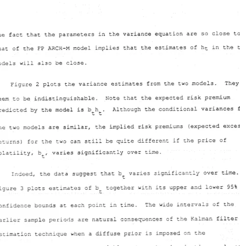
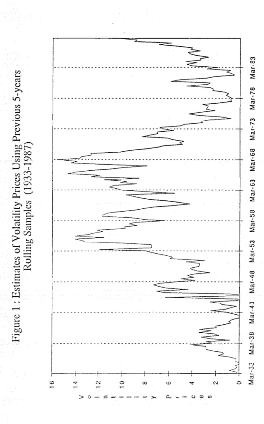
years of weekly data, amounting to approximately 260 observations. The rolling estimation procedure yields a muarterly time series of the coefficient c in (11.5), with _{221 quarterly observations.}

The graph of this _{series in Figure} 1 is _{strongly time—varying.} The

coefficient ranges from —0.4 to 15.6, with a mean of 5.4 and standard

deviation of 4.1. Both the _{dynamic pattern and the magnitude of} the coefficient are similar to the results in Friend and Blume (1975) who report mean/variance ratios of _{0.925, 8.673, 14.165,} and 1.372 for the respective four decades between 1932 and 1971. That is, the ARCH-N

model, which uses the conditional distribution, confirms the instability of the mean/variance ratio. The erratic behavior of this coefficient

indicates the inadequacy of the ARCH—N model to fit the stock return

data.

Another empirical anomaly reported by FOS is that the ARCH-N model

seems _{to predict risk pcemiums} which are too high, with the average predicted excess return almost twice the average realized excess

returns.3 It is hard to accept a _{model that performs so badly in this} respect.

To sum up, although the ARCH-H model is a useful _{tool in modeling} the stock index _{return, adjustments to the model seem necessary. The}

instability of the estimated value for risk aversion end the

inconsistent behavior of excess returns that the ARCH—H model predict are important empirical anomalies that should be resolved.

The _{estimated parameters from} the rolling sample estimation

indicates that a _{time—varying approach may be appropriate. The rolling} sample estimated series _{is only an approximation} because it uses relatively short sample periods (five years is arbitrary), and it is unlikely that quarter to quarter changes of the ooeffioient would be so large. Further, it is inconsistent to estimate _{a time—varying}

parameter, while at the same time assuoting it to be constant within five—year sample periods.

The next section introduces an ARCH-H model with a time-varying mean/variance ratio, which allows formal estimation and explanation of the variation of this parameter.

III. The Time-Varying Parameter ARCH-H Model 111.1 The Model

Consider

the

time—varying parameter

ARCH-H

(henceforth

TV? ARCH-H)

model

5FSS report

the

cx

post

mean

of the

index

return

to

be

0.61%

per

month,

wnile

the average risk premium (the expected excess return predicted) from the ARCH—H model is 1.34%. In other words, the residual terms do not _{sum up to zero} as the model assumes.

y _t

bh

tt

+e

_t (111.1) b

b

+V

(111.2)

t t—s t ht = a0 +

a11

a2h (111.3)

where the _{PARCH surprise veriabie} is

— _Et

The errors

e

end

v

are assumed to be unrorrelated Geussians with sero means and with Variances h and Q, respectively, This model is a

direct extension of the ARCH—H model where the _{parameter characterizing} the mean/Variance trade—off is assumed as a random walk. In the

literature of state space models, (111.1) and (111.2) are called the

-

measurement and the transition eauations; b is called the state t

variable. When h is _{observable, the two equations together} formalise the _{usual time—varying regression} model. As

h

_{measures volatility of}

stock returns, bt measures the increment of the _{risk premium pet} unit of volatility and will be called the "price of volatility" of stock

returns.

In our model, h, is _{assumed to be driven by} a "modified" GARtH (1,1)

process _{specified by} (111.3) .

In

(111.3), the original souared

prediction error,

4_

of

111.6), is replaced by a newly defined

prediction error or "innovation." This replacement is necessary berause both

bt and bt are unobservable. The innovation 1)

is

determined by

= — Et 1(b(h = e +

[b

—

E1(b(]h

(111.4) where

Eti(b(

is the optimal forerast of b given all infonsatior up to time t-l. As Q, the variance of the state variable becomes small, the model converges to the fixed-parameter (FR) ARCH-H model.

11

There are three sets of unknowns to be estimated: b the states;

t,

h, the variances of e; and

a,

2'

a3, and Q, the fixed parameters. The estimation of these unknowns is carried _{out simultaneously by} a Kalman filter and maximum likelihood. Estimates of the states ace produced by the Kalmsn filter conditional on the parameter values. Given values of the parameters, the variance of the measurement errors can be obtained through the BARON equation. After each pass of the Kalmsn filter and the BARON equation, the value of the likelihood can be computed, and nonlinear routines can then be used to maximire the likelihood. These steps are repeated until ccnvergence is reached.4

At each point in time, the contemporaneous variance of (denoted N) is obtained from the valuea of the parameters. The log likelihood function

for

this

model can

be

written

in

terms

of the innovations

(see

Schweppe

(1965)),

as

= . (111.5)

The

quasi

Gauss-Newton

algorithm

is

used

to

maximire

the

likelihood

crcton

Nor-regsta;aty

constraints are

..nposed

on n by

restnctitg

to be non-negative and

l

and

a2

to

be between

3

and

1.

Numerical

The Kslman filter is widely used in systems engineering, It has been applied also to economic models with time—varying coefficients and unobservable components. Basically it is a recursive algorithm that produces optimal estimates of the state variable. It is optimal in the aense that it produces the minimum mean square error estimates of the states, conditional on the newly available information. Anderson and Moore (1971) give a _{comprehensive exposition of Kalman filter methods,}

and Engle and Watson (1985) provide a survey of applications of the Kaimsn filter in economics.

derivatives are _{used to compute the gradient using} the IMSL sub—routine

"EOONF."

Initial values are required for both state and _{variance variables,} b0, h0, as well as for the parameters a. and 0. Values from estimating a Ft (fixed—parameter) ARCN—M are natural candidates for the ai's and

ho, and indeed turn out to be cuite efficient in approaching the final

estimated values. A diffuse prior distribution is assumed for the

initial value of the state, _b0, i.e., we assign a large value (1000) to

its variance.

111.2 Results

The data used for estimation are _{the monthly excess returns} (in percents) of the NYSE value—weighted index for 1926—1985. There are 720 observations. The Ft ARCH—M model estimates (with t—ststistics in

brackets) are: r = 3.OOh e (III.6( 5,0 t t (5.24) h 0.996 +

0.1294.

+

0.835h1

(111.7) (3.40) (5.97) (38.89)

These parameter estimates are used for initial values in estimating

the TVP ARCH-N model. The final converged values for the parameters in

the variance equation, _{a0, a1,} and _a2 are, respectively, 0.989, 0.127,

and 0.836, very close to the estimates in the fixed—parameter model. The estimated value of Q is 0.032, much smaller than that of h _(average

of 31.995). The average vslue of

ht corresponds to a standard deviation of 19.6% per year, which is close to that of Ibbotson _{and Sinquefield.}

13

The fact that the parameters in the variance equation are so close to that of the F? ARCH—N model implies that the estimates of ht in the two models will also oe close.

Figure 2 _{plots the variance} estimates from the two _{models. They} seem to be indistinguishable. Note that the _{expected risk premium} predicted by the model is _bht. Although the conditional variances from

the two models are similar, the implied risk premiums (expected excess ruturna( for the two can still be quite different if the _{price of} volatility,

b, varies significantly

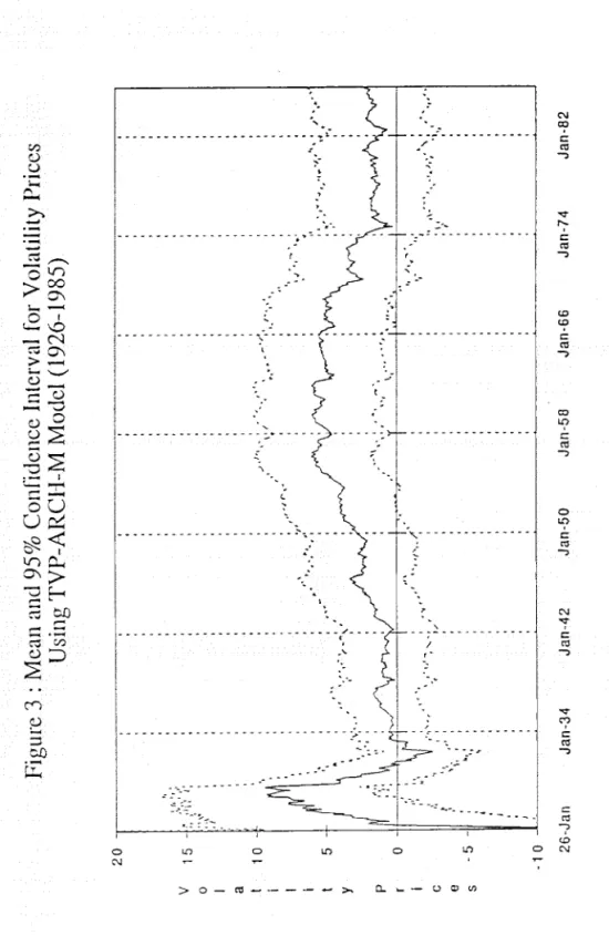
over time,

Inuoed, the data suggesc that _bt varoes significantly over time. Figure 3 _{plots estimates of b together woth} its upper end lower 95% confidence oounds et eacn poont in time. The wide intervals of the earlier sample periods are natural consequences of the Kalman filter ertomation teonnoque wnen a _{diffuse prior} is imposea on the

nitialiration of the state variable. At each point in time, only past i:.forrutocn (which includes the large variance set for the initial state; is incorporated in estimating the state variable. Tmprecise estimates are obtained during earlier periods of the sample, because little information from the data is used, leaving only che effect of the diffuse prior. This phenomenon explains the initial broad confidence onoervals

of

o whi on

gradually

narrow

to

a

reasonsoly

stationary level.

Except

for

the earlier

periods,

b

is

mostly

significantly

positive,

conformong

the

existence of

time—varying

risk

premiums.

For

some

periods the significance levels are greater than

5%,

but

except

for

a few

early

periods the point estimates are

always

positive.

Excluding

the first ten years, b ranges during the five decades _{1936—1985 from}

017

to 5.99 with an _average of 3.04 and standard deviation of 1.68. The averaoe - b

t

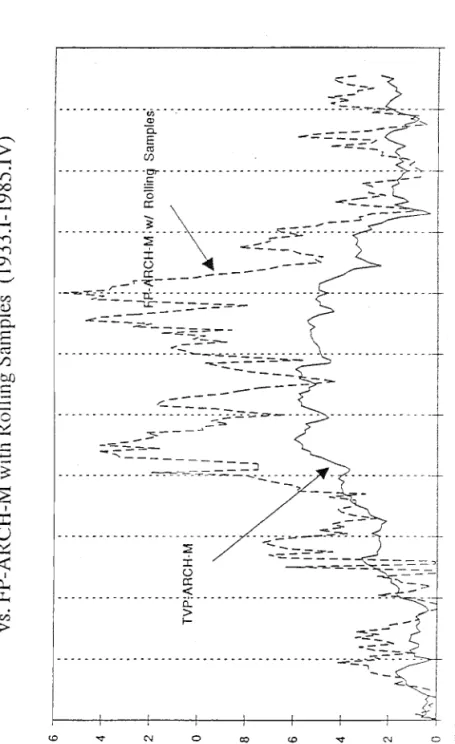
is virtually identical - to the estimate uaino the fixed- paramater model, 1.00.

It's _interesting to comoare this

ht series with the rolling sample

result (see Figure 4) . The general patterns of these two series are ouita similar. _They are _{low in the thirties and gradually increase}

during the forties. _{They remain high during} the fifties and sixties,

then drop hack to a lower level after the oil shocks and recession uf

the mid—seventies. The correlation coefficient of these two series for their overlapping sample perioda (quarterly 1933—1985) is 0.87. The TVP series _{is notably smoother than} the rolling sample estimates, which

suggests that the extreme fluctuat

ma

of the rolling sample estimates

may _{be partly due} to _sampling errors.5

As we noted earlier, although the volatility series from the F? ARCH—N end the TV? ARCH-N models are indistinguishable, the implied equity prer.iuma or the expected excess returns can be quite different,

as is evident from variations in the price of volatility. Comparison of

these two series provides an opportunity to resolve the "puzzle"

reported by FOS that the ARCH—N model gives an average risk premium that is twice as high as the _{average realized} excess return.

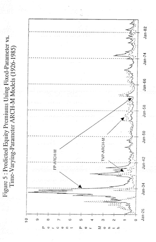
Table 1 shows that the average risk premium for the TV? ARCH—N

model is .54 or .60, depending on the treatment of negative values,

5Some fluctuation in the _{rolling sample estimates may be attributable}

to shifts in parameters in the variance equation that the _{time—varying} parameter model, which assumes _{constancy for all these parameters,}

15

while the F? ARC!{-M _average is .96. The sample average excess return is .64 close to rhe TV?—ARCH-M average risk premium. Figure 5 graphs equity premiums (predicted excess returns) from both models, During

highly

volatile

periuds,

the

fixed-parameter

model seems

to

overestimate

the level of risk

premiums.

For

less

erratic

periods, rhe difference

between these

two

series

is

not obvious,

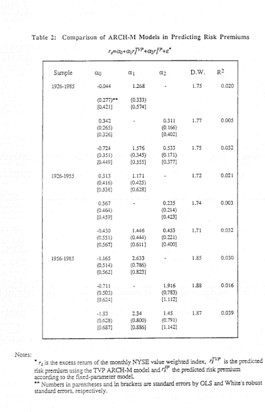
To compare the predictive powers of the two methods, _{we regress the} realired

excess

return

on

each

of the predicted

premiums.

Regressions

with both

predicted

premiums

as explanatory

variables

are

also

eotimated. Table

2

presents the regression

results

for the

full

sample

period

and

for

two sub—periods. Both

ordinary

standard

errors

and

Whotes

consistent, standard

errors are

given.

The R2

of

the

regression

wion a

regressor

from

the

TV? ARCR—M modet

is

significantly

higher than

the regression using

F? ARCH—M

in all

samples.

When

both

regressors are

incicued

in the

reg:ession,

the

premium

predicted

by

the

TV? ARCHM model

has

a higher t-value than

that

predicted

by

the

fixed parameter

model

in all

samples.

IV.

Explaining Variationa

in the ?rioe

of

Volatility

IV,1

Economic

Variaoles Affecting

the

Price

of Volatility

Application

of

a TV? ARCW—M model

appears

to correct

the biased

forecasts

of

risk

premiums

that

are generated

by

the

F? ARCH—M

model.

Hecc we try to explaIn variations in 5 , estimates

of

the price

of

t

volatility,

by

examining

its

relation

with

some macroeconomic

variables

under

the

assumption

that

the

true

model

is

a CA?M

with

a

constant

price

of risk. As b is the mean/variance ratio of the stock-index excess

catucn, dividing both sides of (11.3) by

o

yields

b_ = S[wt +

(l_)3ll]

_)IV.l)

The

sensitivity

of the _{return on the unobserved portfolio to} the retucns

of

stocks,

that

is,

the

beta

coefficient

of the

unobservable

sssets

_on

the

stock index is

Letting

B

and

3

be

tirLe varying,

bt

3Ct

+

(lwt)N

)IV.2)

Thus,

the

price

of

volatility

of stock returns

depends not only

on

the

risk

aversion

parameter,

3,

but

is

also affected

by

the

poctfolio

weight

w

and

the sensitivity

psrameter

.

b

will

be

identicsl to

3

in

two

extreme

oases:

w1

or

=l,

We

use

_economic

variables

that

proxy

changes in

'

and

3

to test the velidity of the TUg model in explaining variations in the price of volatility.

Inferences about the CAPM are sensitive to the set of assets used

in the test. Stathaugh (1982) examines the effect of moving from narrow

to broader stock indexes. But even if we could compile an index of

dl

I the incorporated enterprises in the U.S., it would account for less then

10% of wealth if we included human carital, and less than one third of

I the total wealth of U.S. _{citirens excluding human capital} (See Ibbotson

end Erinson _{(1987, ppp.18—3S)} ) We choose to treat the aggregate of all

essets _{other than equities as the unobservable complement of total} wealth -

17

We use four different proxies for

w.

The first two proxies are the broadest in that they refer to all U.S. assets; real (including numan capital), and financial. The flow of income from ownership of stocks _{is approximately measured by corporate profits while the income} from all wealth is simply national income. If each is 1(1), and each is discounted at the same rate, their ratio will approximately equal the ratio of the value of stocks to total wealth. Hence the share of corporate profit in national,

w1, income is a possible proxy for w.

The second proxy, _w2, is the ratio of the value of all NYSE stocks to gross consumption. The _{single—factor} OAPN with a constant

cpportunity set (which is equivalent to the consumption beta model) imploes chat changes in gross oonsumption reflect changes in total wealth, ht best, tins measure tan only be proportional to the share of equities in total wealth. Both consumption figures and the value of NYSE stocks are available monthly from 1959 to 1985; quarterly observations are iveilable from 1946 to 1985.

Two more proxies for w correspond to narrower definitions of wealth. For

w3, total wealth is am estimate of physical wealth which

includes all financial and tangible assets for the total U.S. economy, while for

w4 only financial assets are included. Total equity value is used for tne numerator instead of the aggregate value of NYSE-listed stocas.6 Tnese nate come from the "Balance Sheets for the U.S. Economy"

(1987, published by the Federal Reserve Board. Only annual observations are availaole,

6 As of Oeoember 1985, the total value of stocks listed on the NYSE was about 79% of the value of all U.S. corporate equity.

eatate. There is little doubt that the beta of real estate on storks is less than one, indeed, it may very well be negative (See Ibbotson and

Brinson (1987, pp.35—43)) . The beca of human _capital on storks is also

must likely small. While business ryrles affect labor income and

corporate

profits

similarly,

they

affect

highly

skilled

labor less

than

unskilled labor.

Indeed, investment

in

human

capital

_may

very

well

be

counter cyclical. While it is impossible to compute 3,.

directly,

time-

varying elements of i may be captured nevertheless by eccncrdr

variables, We use the rate of inflation and the reel interest rate. It

is plausible that: the sensotlvicy of wealth—asset prices to the prices

of _{stocks differ In period} of different levels of inflacion and real

interest rates.

The third source of variaticns in b comes from

'

the

risk

eversion parameter. For a broad class _{of stylized utility} functions, e.g., tIARA, relative risk aversion will depend on the level of wealth,

and ccnseouently may be correlated with changes in the level of

consumption. There

is neither

evidence mcr

stylized fact

on whether

relative

risk

aversion

is

increasing,

decreasing, cc

constant

in

wealth,

although it is a stylized fact that absolute risk aversion decreases with wealth (see Wachina (1987) ) ,

IV.2

Correlacioo of

bt

with

Eccncmic Variables

Table

3 _{presents regressions} of _{b_} cmi h,, on the four proxies for

the stock—portfolio weight, the two economic variables that are expected

19

rate of interest and the rate of inflation), and the instrument for risk aversion (real per-capl.ta consumption) . We report results for the value

ieighted series only, since

they

are almost identical to the equally weighted series. All the variables in Table 3 are estimated to be 1(1), and hence differenced. These estimates are approximations for the variables in equation (IV.2) and are estimated with quarterly data.

The economic variables, particularly the proxies for the relative portfolio shares of stocks, are, by design, contemporaneously correlated with the stock returns. As a _{result they will also be highly correlated} with the estimated b and, but not with the h series. To minimize the

t t

effect of this spurious correlation, the second panel of Table 3 presents identical regressions with lagged values of the economic variables. Each panel in Table 3 presents estimates from three

regressions on the economic variables, two for the price of volatility and one for the volarility itself. The first regression of the price of volatility excludes the volatility itself, the second includes it.

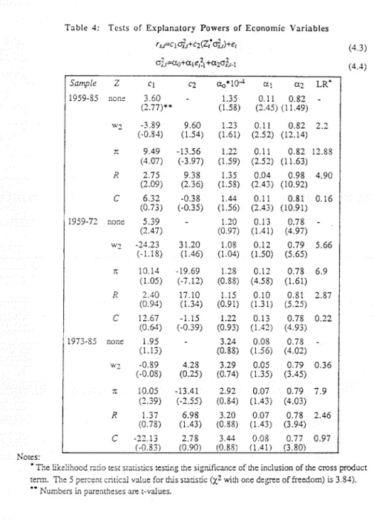
The regression results clearly support the hypothesis that the price of volatility can be varying due to changes in the relative value of stocks, and the beta of unobserved assets, even if risk aversion remains constant. The next to last row of Table 3 gives the X2

I

statistic

(with 4 degrees of freedom) for the hypothesis that the coefficients of all _{four proxies} for portfolio share of stocks are zero. The critical value for z.OOl is 14.85, while the test statistic is greater than 30 in all four regressions.

The positive coeffioient of all

w's

is consistent with (IV.2) for

bets less thsn one. When the value of stooks rises relative to other

oomponents of wealth, a rise i: the price of volatility oan be attributable to the increased marpinal risk of storks, rather than to higher risk aversion, At the sane tine, the variance of the rate of return of stooks _{is attually} lower, as suggested by the negative coefficients of the proxies (in 7 out of 8 oases) in the regression of conditional variance on the economd,c variables (and as might be predirted by a _{leversge argument)}

Both _{proxies for} the beta of unobserved assets with stocks, the rate of inflation and the real rate of interest, _{have a significant}

(negative) impact on the price of volatility. Equation Iv,2 predicts that bets _{will be negatively correlated with the price of volatility.}

0cc results agree if we assume that the beta of unobserved assets on stocks is greater in periods of high inflation and real interest rates.

Real per—capita consumption, the proxy for the coefficient of risk aversion, shows a

contemporaneous

strong

(negative) impact

on

btf

and

hardly

any impact: when

lagged

one

q-uarter.

With

constant

relative risk

aversion, the

result

of the

contemporaneous

regression

is attributable

to

the positive

correlation

of

changes

in

consumption

with

changes

in

wealth, and hence with

rates of

return

on

stocks.

The

absence

of

significant

impact

of

consun.ption

in

the lagged eqvation

is

consistent

with

this

explanation.

On

the other

_hand,

if

taken

at

face value, the

positive coefficient of

consumption

in the

contemporaneous

regression

suggests that

risk

aversion

is

increasing with

wealth. Risk

aversion

21

The results presented in Table 3 make a case for our argument that

C

risk

aversion may not easily be inferred from rates of return on stocks

and

that

economic

variables affect

the

price

of

volatility.

IV.3

Further Tests of

the

Dependence

of

b

on Economic Variables The

regression analysis

so

far

has been

descriptive since

it

uses

as

dependent variable estimates from the entire sample. We now

substitute (17.2) for (111.2) and recognize that the economic variables must interact with the volatility. If only a single variable is

relevant, the model becomes

r5

=

c,,t

+

c2(,t1

+

e0

(17.3)

2 2

=

a0

a,ts,t_l

+

a2O,t_l

(17.4)

where

r is

the

excess

return

on

stocks,

and

is

one

of

the proxies or

related

variables of w,

,

and 5.

This

is

the ARtH—M model with cross— product

terms

in

the

mean

eruation,

and can be estimated

by maximum

likelihood.

Monthly

data

are

used

for

formal

tests

on

the significance of

the

coefficient

_c2

because

higher

freouency

data

provide

better

estimates of

conditional

variances. The sample covers the period 1959-1985,

corresponding

to

the

availability

of

the

consumption

data. Estimation

results

are also reported for sub sample periods 1989—1972, and 1973— 1985. Table 4 _{presents the} results.

Except

for

per

capita real

consumption,

estimatiot.

results

support

variables, consistent with the regression result of Tatle 3, Once the

cross

product term

w2C,

is included in the model, the coefficienc of

becomes insignificant and even assumes the wrong sign. The low t—

statistic

values of the coefficient of _{the cross—product} term may

reflect multicollinearity. Estimation with _{only the cross-product} term yields a t-statistic of 2.82 for _{the full sample,} with 2.8? and 1.00 for

sub sample periods.

The

role

of

inflation

appears

to be

the

most

important.

When ohe

inflation

rate

is

used

for

I in the

estimation, the

t—valueo

of

izC

are

always

significant

at

the

5%

level.

In

an attempt to

estimate a

structural

model we assume

that the

sensitivity

factor,

'

is

linearly

dependent

on

the rate of inflation,

i.e.,

_A0 +

A1it, and

that

the

stock return

is

driven

by

_a

process

with

mean given by (11.3) with a _{GARCN)l,1) variance specification.} The

model

can

then be written as

r50

= S[w_1 +

A0(l

—

w1)

+ A1(1

— _w

1)r11,c

+

e

IV.t)

=

a0 +

a1e1

+

a2,t1

(IV.6)

Ecuation (IV.5) can

also

be

rewritten as

r5

=

C1w_,,t

+

C2(l

—

w1),t

+ C3(1 —

w1)r.,t

+

e

(17.7)

where

C1=

C2=A03,

and

C3=A16, Note that all explanacory economic variables _{are lagged once to ensure} that the _{expected return depends}

23

measured by the ratio of corporate profit to national income becauoe it is available from 1946.

It turns out that very large standard errors are obtained for estimates of _C1 and C_. The reason is that

w

is very smooth compared with so the collinearity between and

(l—w1),t

is high. The model is also estimated assuming _A3=1, i.e,

=l±Alrt implying

CrC2

and

that equals one wich no inflation. Table S gives the

results,

including estimation

with

wl,

wnicn corres

onds

to the

usual

fixed-parameter

ARCh-k

model.

As

the

likelihood function values

indicate,

both

models

witn and

without

unit restriction

for

_A3

outperform

the usual

ARCH—k

modei.

The

restricted

version

(Al)

cannot be

rejected

and reduces

the

standard

error of

the coefficient

C1,

which

is

also

an

estimate of

the risk

aversion parametar

& In

this

procedure,

the point estimate of

this

parameter

becomes positive for the full period and toe second sub sample period. The estimates of C, and C, are reasonably stable across the two

sub sample periods, although both are less significant for the period 1966—1985. The likelihood ratio test for _{model stability across sample} periods suggests that the restricted model is stable, wnile the fixed— parameter ARCH—k model is not.

To investigate the robustness of our model we perform some fortoer diagnostic tests. We have restricted our variance specification to GARCH(1,1). Sut there are no theories to exclude other economic variables _{that may be} important in driving the conditional variances as well as the conditional mean. It is possible therefore that the effects

of econoric variables on the _{price of volatility are attributable} to

this relationship through the second moment.

Researchers who follow thia strategy in modeling stock variances

include Campbell and Shiller (1989), Harvey (1989), Attanasio (1989), and Attanasio and Wadhwani (1989) among others. Abtanaaio and Wadhwani

(1989) ,

for

example, find that the predictability of expected stock

returns given lagged dividend yields reported in Fama and Frenob (1988) can _{be explained by a} risk measure estimated by an ARCH with laooed dividend _yields.

We hence re-estimate our final model (with the restriction

A6=l) while allowing lagged inflation rates _{and lagged portfolio} weights to

enter into the variance egustion.

A

likelihood ratio test of our

original model against this general model gives a test statistic of 8.88, which is _significant at the 5% level but not at the 1% level This result indicates that a better forecast of the volatilities may be obtained by including economic variables in the GARCH)l,l) model.

Cur original conclusion concerning the mean effect, however, is not

much affected by thom re—estimation. The estimates of

C1 and C are 7.32 (with t—value of 4.92) and —7.04 (with t—value of —3.26), which are

fairly close to the riginsl estimates in Table 5. Further, the

significance of the two economic variables

(w2 and m) added to the variance _equation is _{weaker according to the Wald test} )t—values 1.67 and _{—0.75, respectively,} not significant at the 5% level) -

According to the result of the restricted model for the foil sample

25

most likely too hIgh. The two standard error low bound for this parameter is 4.67, which is more in acrord with other estimates.

V. Conclusion

Analysis of an econometric model estimating a time—varying risk! return relation of the stock market indicates that the TVP ARCH—M model provides more precise estimates of the expected return of the stock market index than the fixed—parameter ARCH-k model. The model takes explicit account of the role of risky assets other then stocks in explaining the time variation of the mean/variance rstio for stooks. Proxies for portfolio weights end the bets of the unobserved assets on stocks

are

found to he

tmoortsnt

in

deterraning expected stock

returns.

Although oor

oeoi

noel

work

is

only

nreliminsry,

further studies

in

this

vein

seem

promising.

More

detailed investigations

may

explain

the

role

of

the

rate

of

inflation

in

stock prioe

movements. The

relationship

of

our

findings

with

the recent

literstuoe

on

predictability

of

excess

stock returns

may

be

fruitful

for future

Appendix: Notatcn

rM : excess return of the market portfolio total return —

rf

: riskless rate

r5 : excess return of a comprehensive stock index

excess

return of the

unobserved

risky

asset

other than

stocks

w :

portfolio

weight

of stocks

in the

market

portfolio

(or

the

relattve

demand

for storks)

proxies for

w

corporate

profit/national

income

total

NYSE

value/gross

consumption

toral

stock value/value of

total financial assets

tangible

assets

total

stock value/value of

total financial assets

sensitivity

of returns of the unobserved risky asset to stocks =

Cov(r

_{,r )/var)r}

N S S

m :

inflstioo

rate

measured by

the

Consumer

Price

Index

R : real interest rate =

r

— St

C : real _{per capita consumption}

b : _{time—varying}

parameter measuring

price of

volatility

of

stocks

27

References

Acel, A. 1988, "Stock _{Prices Under Time Varying Dividend Risk} : An Exact

Solution In An Infinite-Horizon _{General Equilibrium Model,"} Journal of Monetary Economics, 22, pp.375—393.

Akgiray, V., 1989, "Conditional Neteroskedasticity in Time Series of Stock Returns: Evidence end Forecasts," Journal of Business, 62,

55—80.

Anderson, B. and J. Moore, 1971, Optimal Filtering, Prentice Mall, Inc., Englewood Clifts, N.J.

Attanasio, 0., 1989, "Risk, Time Varying Second Moments and Market Efficiency," Manuscript, Stanford _University.

Attanasio, 0. and S. Wadhwani, 1989, "Risk and the _{Predictability of} Stock Market Returns," Manuscript, Stanford University.

Backus, D. and A. _{Gregory, 1988, "Theoretical Relations} Between Risk Premiums ani crrilitional Variances, " Manuscript, Federal Reserve Bank

of

_Minneapc- Li 5

Balance

Sheets

for

the

U.S. Economy, 1987, Board

of

Governors

of

the

Federal Reserve

System.

Black,

F., N. Jensen, and N. Schuies, 1972, "The Capital Asset Pricing Model: Some Esipirocal Tests," in N. Jensen, ad., Studies in the

Theory of Capital Markets. Praegar, New York, 79—124.

Bodia, 1., A. Kane, and R. McDonald, 1983, "Mhy Are Real Interest Rates So Nigh?" NBER Working Paper No. 1141.

Bollarslav, Tim P., _tn, "generalized Autoregressive Conditional Neteroscadastici':y, "

Journal

of Econometrics, 31, 307—327.

Bollarslev, T., R, Chou and K. Kroner, 1990, "ARCH modeling in Finance: A Review of the Theory and Empirical Evidance," Journal of

Econometrics, thLs issue.

Campbell, J. and R. ihLller, 1989, "The Dividend Price Ratio and Expactations of t'utura Dividends and Discount Factors, " Review of Financial

Studies,

195—228.

Chou, R. _{Y., 1983 "Vniatility Persistence} and Stock Valuations," Journal of _{Applied Euoncmatrics,} 3, 279—294.

Conn R., N. tawetien, K. Lease and 0. Schlarbauxs, 1974, "Individual Investoc Risk Aversion and Investment _{Portfolio Composition,"} Journal of Finance, 30, 603—620.

Engle, R. F., 1982 _{"Autoregressive} Conditional Nataroscadasticity with Estimates of tne Variance of U.K. Inflation," Economatrica, 50, 987—1008,

Engle,

R. F., D. tilien and R. Robins, 1987 "Estimating Time Varying Risk

Pramia

in

the

Term

Structure:

The ARCH-N

Modal,"

Engle, R. F., and M. W. Watson, 1985 "Applications of Kalman Filtering in Economics," Paper presented at the World Congress of the Econometric Society.

Epstein, L., and S. Sin, 1989, "Substitution, Risk Aversion and the Temporal aehavior of Consumption and Asset Returns: A Theoretical Framework," Econometrica, 57,4, 937—969.

Fama, E., and K, French, 1988, "Dividend Yield and Expected Stock Returns," Journal of Financial Economics, 22, 3—26.

Fam.a, E., and J. MacBeth, 1973, "Risk, Return and Eiilibrium: Emmiriosl Test," Journal of Political Economy, 607—636. French, K. R., C. Schwert, and R. Stambaugh, 1987 "Expected Stock

Returns and Volatility," Journal of Financial Economics, 19, 3—30. Friend, I., and N. i3tume, 1975, "The Demand for Risky Assets," .Roerioon

Economic Review, 65, 900—922.

Glosten, L., R. Jagaunathan and D. Runkle, 1989 "Relationship Between

the

Expected Value

and

the

Volatility

of the

Nominal

Excess

Retuot

on

Stocks,"

Manuscript, Northwestern

University.

Grossman,

S,

and

C.

Leroque,

1987

"Asset

Pricing

end Cptimal

Portfolio

Choice

in the Presence of Illiquid Durable Consumption Goodt," USSR

W.P. No. 2369.

Marvey, C., 1969, "tn the Expected Compensation for Market Voletility

Constant Through Time 7" Manuscript, Duke University.

Tbbotson, R. C. end C. Brinson, 1987 Investment Markets, McGraw—Hill

Book Co.

Keim, D. 1986, "The CAPM and Equity Return Regularities," Financial Analyst Journal, May—June, pp.19—34.

Lintner, J. 1965, "The Valuation of Risky Assets end the Selection of

Risky Tnvestments in Stock Portfolios _{end Capital} Budgets," Review of Economics and Statistics, 47, 13—37.

Machine, N., 1981, "The Economic Theory of Individual aehevior Toward

Risk: Theory, Evidence, and New Directions," Manuscript, UCSO. Mankiw, N., end N. Shapiro, 1986, "Risk and Return: Consumption versus

Market Pete," Review of Economics and Statistics, 68, 452—459.

Merton, R. C., 1913, "An Intertemporal Capital Asset Pricing Model,"

Econometrica, 41, 867—887.

Merton, R. C., 1960, "Cn Estimating the Expected Return on the Market,"

Journal of Financial Economics, 8, 323—361.

Mossin, J., 1966, "Squllibrium in a Capital Asset Market," Econometrics,

29

Pindyck, R. S., 18U, 'Risk Aversion and Determinants of Stock Market Behavior,' The Review of Economics and Statistics, LXX,2 pp.l53— 190.

Pratt, J.W., 1964, "Risk Aversion in the Small _{and in the Large,"} Econometrica, _{32,1—2 pp.122—136}

Roll, R., 1977, "A Critique of Asset _{Pricing Theory's Tests: Part I,"} Journal

of

Financial _{Economics, 4,} 129—176.

Schwepe, F., 1965,"Evaluation of Likelihood Functions for Gaussian Signals," I.E.E.E. Transactions on

Information

Theory, 11,

61—70.

Sharpe, W., 1964, "Capital Asset Prices: _{A Theory of Market Equilibrium} Under Conditions of Risk," Journal

of

Finance,

19,

425—442.

Stambaugh, R., 1982, "On the Exclusion of Assets From Tests of the Two— Parameter Model," Journal

of

Financial _Economics, 10, 237—268 Tobin, J., 1958, "Ltquidity Preference as Behavior Toward Risk," Review

Risk Premium Mean Std Dcv Minimum Maximum

064

560

-29.03 38.16

rT

0.54 0.63 -3.51 4.73

r'

0.60 0.47 0.00 4.73 0.96 1.28 0.24 9.86 Notes:

rI"

is the predicted dsk premium using the TV? ARCH-M model, and

rif

the

predicted risk premium according to the _{fixed-parameter model}

Table 2: Comparison

of

ARCH-M Models in Predicting Risk Premiums r_—ci.o+alrT"+a2rff+e Sample

ao

D.W. R2 1926-1985 -0044 1.268 - 1.75 0.020 (0.277)* (0333) [0.421) [0.574) 0.342 - 0.311 1.77 0.005 (0265) (0.166) [0326) [0.402) -0.724 1.576 0.533 1.75 0.032 0351) (0345) (0.171) [0.449) [0.555) [0.377) 1926-1955 0313 1.171 - 1.72 0.021 (0416) (0.425) [0.538) [0.628) 0.567 - 0.235 1.74 (0.464) (0.214) [0.459) [0,423) -0.430 1.446 0,453 1.73 0.032 (0.551) (0.444) (0.221) [0.567) [0.611) [0.400) 1956-1985 -1.165 2.633 - 1 85 0.030 (0.514) (0.786) [0.562) [0.823) -0.711 - 1.916 1.88 0.016 (0.503) (0.783) [0.624) [1.112) -1.53 2.34 1.45 1,87 0.039 0.62S) (0.800) (0.791) [0.6871 [0.886) [1.1421 Notes:

r4 is the excess return of the monthly NYSE value weighted index,

rT'

is the predicted

risk premium using the TVP ARCH-M model and

rff

the predicted risk _premium according to the _{fixed-parameter modeL}

Numbers in parentheses and in brackets are standard errors by OLS and Whites robust standard errors, respectively.

With _{contenporaneous With explanatory}

explanatory variables variables lagged one period Dependent

b'R

b'R

h'WR bt'WR b''wR

h'R

variable wI 3.92 3.89 -10.77 4.77 5.02 -79.48

(i.75)

(1.73) (-0.14) (1,22) (1.33) (-1.04) W2 3.05 3.06 4.48 0.74 0.69 -38.32 (14.51) (1455) (0.60) (2.00) (1.91) (-5.26) W3 -4.59 -4.88 -111.48 1.21 2.56 -6.39 (-1.55) (-1.65) (-1.06) (0.24) (0.52) (-0.06) W4 10.27 10.10 -63.50 7.66 8.74 -15.96 (3.30) (3.24) (-0.58) (1.43) (1.68) (-0.15)

n

-0.11 -0.12 -3.14 -0.28 -0.24 2.11 (-2.19) (-2.33) (-1.78) (-3.22) (-2.79) (1.22) R _{-0.13 -0.14 -2.85 -0.29 -0.25 2.46} (-2.48) (-2. 61) (-1.53) (-3.10) (-2.74) (1.36) C 0.60 0,54 -24.81 -0.65 -0.34 -3.81 (2.65) (2.28) (-3.08) (-1.69) (-0.88) (-0.51) 6VWR - _-0.003 - - _0.01 - (-1.08) (3.25) CONST. -0.04 -0.03 0.93 0.01 0.003 0.14 (-2.57) (-2.36) (1.93) (0.60) (0.12) (0.30) R2 0.77 0.78 0.24 0.30 0.35 0.28 D.W. 2.21 2.21 1.85 2.03 2.09 2.03

y2(4)**l0535

104.13 15.65 32.23 39.64 35.19

p-vue

<0.01% <0.01%

<1%

<0.01% <0.01% <0.01% Notes:

Wj'S are _poro1io shares

of

stocks with different weaith measures, tt is the inflation rare,

R is _{the real interest rate, and} C is the real _{per capita consumption in thousands}

of

dollars. The sample period is quarterly 1951.1- 1985W with 140 observations. All variablcs in

the regressions are

flrt

differenced. Numbers lit _{the parentheses are t-values.}

x2(4) is the test statistic for the _{joint hypothesis that all coefficients} for Wj5, i =

Table 4: Tests

of

Explanatory Powers of Economic Variables (43) (4.4) Sample

Z

cj c2

a1O4

a

U7

LR

1959-85 none 3.60 - _{1.35 0.11 0.82 -} (2.77)** (158) (2.45) (11.49) W2 -3.89 9.60 1.23 0.11 0.82 2.2 (-0.84) (1.54) (1.61) (2.52) (12.14)

z

9.49 -13.56 1.22 0.11 0.82 12.88 (4.07) (-3.97) (1.59) (2.52) (11.63) R 2.75 9.38 1.35 0.04 0.98 4.90 (2.09) (2.36) (1.58) (2.43) (10.92) C 6.32 -0.38 1.44 0.11 0.81 0.16 (0.73) (-0.35) (1.56) (2.43) (10.91) 1959-72 none 5.39 - 1.20 0.13 0.78 - (2.47) (0.97) (1.41) (4.97)

w

-24.23 31.20 1.08 0.12 0.79 5.66 (-1.18) (1.46) (1.04) (1.50) (5.65)

t

10.14 1969 1.28 0.12 0.78 6.9 (1.05) (-7.12) (0.88) (4.58) (1.61) R 2.40 17.10 1.15 0.10 0.81 2.87 (0.94) (1.34) (0.91) (1.31) (5.25) C 12.67 -1.15 1.22 0.13 0.78 0.22 (0.64) (-0.39) (0.93) (1.42) (4.93) 1973-85 none 1.95 - 3.24 0.08 0.78

-

(1.13) (0.88) (1.56) (4.02) w-' -0.89 4.28 3.29 0.05 0.79 0.36 (-0.08) (0.25) (0.74) (1.35) (3.45) z 10.05 -13.41 2.92 0.07 0.79 7.9 (2.39) (-2.55) (0,84) (1.43) (4.03) R 1.37 6.98 3.20 0.07 0.78 2.46 (0.78) (1.43) (0.88) (1.43) (3.94) C -22.13 2.7g 3.44 0.08 0.77 0.97 (-0.33) (0.90) (0.88) (1.41) (3.80) Notcs: *

The likelihood ratio test statistics _{testing the significance}

of

the inclusion

of

the cross product term. The 5 percent critical value for this statistic (y2 with one degree of freedom) is 3.84).

Sample

Cj

C2 C3

a104

i

az

lLkelihood 1946-85 -5.6 9.5 -9.0 1.27 0.09 0.83 -1331.23

(.012)*

(1.54) (-3.34) (1.78) (2.67) (13.00) 7.81 - -8.69 1.27 0.09 0.83 -1331.26 (4.98) (-3.61) (1.98) (2.69) (13.08) w=1 4.62 - - 1.47 0.09 0.82 -1337.32 (4.12) (1.74) (2.63) (11.46) 1946-65 110.8 -4.7 -7.5 1.63 0,10 0.76 -633.00 (0.96) (-0.28) (-2.02) (1.05) (1.45) (4.38) 9.81 - -7.96 1.69 0.10 0.76 -633.34 (4.77) (-2.19) (1.03) (1.41) (4,16) w=i 7.96 - - 2.22 0.13 0.69 -636.07 (4.19) (1.23) (1.65) (3.47) 1966-85 -119.7 20.2 -9.9 2.06 0.08 0.82 -693.10 (-1.59 (2.26) (-2.22) (1.22) (1.78) (7.43) 6.22 - -8.35 2.07 0.08 0.82 -694.63 (2.04) (-1.92) (1.20) (1.77) (7.50) w=1 2.2 - - 2.37 0.07 0.81 -696.16 (1.52) (1.13) (1.83) (6.37) Notes:

Monthly data are used, wtl is the rado of corporate profit over national income, rnd7r41 is the inflation rate measured by CPI.

16 14 V 0 _I 12 a _i 10 8 y

P6

c

4 e S 2 0

Figure

1:

Estimates

of

Volatility

Prices

Using

Previous

5-years

Rolling

Samples

(1933-1987)

Mar-33 Mar-38 Mar-43 Mar-48 Mar-53 Mar-58 Mar-63 Mar-68 Mar-73 Mar-78 Mar-83

s 450

q 400 5;

o 350

P 300

C 250

0 n 200 P 0 M

0

n h 150 100 50 0

Figure 2 Volatility Estimates Using

Fixed-Parameter vs. Time

Varying Parameter ARCFI-M Models (1926-1985)

Jan-26 Jan-34 Jan-42 Jan-50 Jan-50 Jan-66 Jan-74 FP-ARCH-M

Figure

3

:

Mean

and

95%

Con!dence

Interval

for

Volatility

Prices

Using

TVP-ARCH--M

Model

(1926-1985)

20

—

—______________

V 15 o

:

: a I 10 I

__

_

26-Jan Jan-34 Jan-42 Jan-50 Jan-58 Jan-66 Jan-74 Jan-82

V 0 a y p C 0 S

Figure 4 Estimates of Volatility Prices Using TVP-ARCI-l-M Model

8 P

nO

C 0 C 7 6

PS

e 10

Figure

5

:

Predicted

Equity

Premiums

Using

Fixed-Parameter

vs.

rfiIe.varyiIgparaI11cter

ARCH-M

Models

(1926-

1985)

4 M

0

n 1 2 8 0 Jan-26 Jan-34 Jan-42 Jan-50 Jan-SO Jan-66 Jan-74 Jan-82