A novel clustering algorithm based on mathematical morphology for wind power generation prediction

This is an Open Access document downloaded from ORCA, Cardiff University's institutional repository: http://orca.cf.ac.uk/118236/

This is the author’s version of a work that was submitted to / accepted for publication. Citation for final published version:

Hao, Ying, Dong, Lei, Liao, Xiaozhong, Liang, Jun, Wang, Lijie and Wang, Bo 2019. A novel clustering algorithm based on mathematical morphology for wind power generation prediction.

Renewable Energy 136 , pp. 572-585. 10.1016/j.renene.2019.01.018 file Publishers page: http://dx.doi.org/10.1016/j.renene.2019.01.018

<http://dx.doi.org/10.1016/j.renene.2019.01.018> Please note:

Changes made as a result of publishing processes such as copy-editing, formatting and page numbers may not be reflected in this version. For the definitive version of this publication, please refer to the published source. You are advised to consult the publisher’s version if you wish to cite

this paper.

This version is being made available in accordance with publisher policies. See

http://orca.cf.ac.uk/policies.html for usage policies. Copyright and moral rights for publications made available in ORCA are retained by the copyright holders.

A novel clustering algorithm based on mathematical morphology

for wind power generation prediction

Ying Hao 1_{, Lei Dong} 1,1_{, Xiaozhong Liao}1_{, Jun Liang} 2_{, Lijie Wang}3 _{, Bo Wang}4 1_{Department of Automation, Beijing Institute of Technology, China}

2_{School of Engineering, Cardiff University, UK}

3_{Department of Electrical Engineering, Beijing Information Science and Technology University,}

China

4_{State Key Laboratory of Operation and Control of Renewable Energy & Storage Systems, China}

Electric Power Research Institute, China

Abstract: Wind power has the characteristic of daily similarity. Furthermore, days with wind power variation trends reflect similar meteorological phenomena. Therefore, wind power prediction accuracy can be improved and computational complexity during model simulation reduced by choosing the historical days whose numerical weather prediction information is similar to that of the predicted day as training samples. This paper proposes a new prediction model based on a novel dilation and erosion (DE) clustering algorithm for wind power generation. In the proposed model, the days with similar numerical weather prediction (NWP) information to the predicted day are selected via the proposed DE clustering algorithm, which is based on the basic operations in mathematical morphology. And the proposed DE clustering algorithm can cluster automatically without supervision. Case study conducted using data from Yilan wind farm in northeast China indicate that the performance of the new generalized regression neural network (GRNN) prediction model based on the proposed DE clustering algorithm (DE clustering-GRNN) is better than that of the DPK-medoids clustering-GRNN, the K-means clustering-GRNN, and the AM-GRNN in terms of day-ahead wind power prediction. Further, the proposed DE clustering-GRNN model is adaptive.

Keywords: wind power prediction; clustering algorithm; dilation and erosion; mathematical morphology; the number of clusters

1

Corresponding author at: 5 South Zhongguancun Street, Haidian District, Beijing 100081, China.

1 Introduction

Wind power is currently attracting increased attention globally as a renewable and clean source of energy. However, because of the intermittency and randomness of wind power, accurate wind power prediction is crucial to ensure the transient stability of the power grid [1]. Accurate wind power prediction can also increase the marketing power of wind producers [2, 3]. The various wind power prediction methods can be classified into three categories: physical methods, statistical methods, and intellectual learning methods [4-6]. Physical methods are based on the topography of the plant. Statistical methods are driven by historical data modeling approaches [7-9], such as Kalman filter [10], and ARMA modeling [11]. Intellectual learning methods establish a nonlinear relationship between the input data and the output power by employing an artificial intelligence approach [12-15], such as artificial neural networks [16-18], support vector machine [2], or hybrid statistical models [19-21].

It is well known that wind power generation fluctuates with weather conditions [22], particularly wind speed and direction. Seasonal changes and the alternation of day and night result in certain days having similar weather conditions. Besides, in meteorology and climatology, a method of forecasting based on finding past occasions that are analogous to the current weather situation, called "Analogue Method (AM)", has a history of more than 20 years [23-25]. Meanwhile, these days with similar meteorological phenomena also have similar wind power variation trends [26]. Therefore, choosing such historical days whose numerical weather prediction (NWP) information is similar to that of the predicted day as training samples can improve the wind power prediction accuracy and reduce the computational complexity during model simulation.

Clustering algorithms are an effective tool in this area [27]. Clustering refers to the process of dividing a dataset into several categories according to the similarity and distance between the data without information a priori [28-30]. Because there are no prior assumptions about the number and structure of clusters, clustering analysis is an unsupervised learning method [31, 32]. Existing clustering algorithms predominantly include hierarchical based clustering, partition based clustering, density based clustering, grid based clustering, or model based clustering techniques [33, 34]. However, most of these algorithms need to specify the number of clusters, k, in advance, and determining k is very difficult. Zhou et al. [35], Wei et al. [36] and Řezanková and Húsek [37] found k by setting a clustering validity value, and using the merge or split rule to increase or decrease k to its optimal value. Sun et al. [38] obtained a series of eigenvalues via spectral decomposition of the data affinity matrix, and then used eigenvalue difference analysis to determine k. Zhang et al. [39] determined k and the initial cluster centers by identifying high-density regions using Neighbor Sharing Selection (NNS). Xie et al. [40] determined k by constructing a decision map of sample distances relative to sample densities. Muneeswaran et al. [41] proposed a method that does not need to specify k in advance, instead it automatically obtains k during clustering.

This paper proposes a novel clustering algorithm based on dilation and erosion (called the DE clustering algorithm) that can automatically determine the number of clusters, k. In the DE clustering algorithm, the sample dataset is processed into a binary matrix that is then dilated and eroded to obtain a new matrix. The number of clusters, k, is then determined by classifying the connected data points with value “1” in the new matrix. Finally, the sample dataset is divided into k clusters by calculating the distance between each data and the cluster centers, which are the mean values of the data in the obtained clusters. The number of clusters, k, is obtained automatically, and the proposed algorithm classifies the sample dataset without supervision. The feasibility and efficiency of the proposed algorithm have been verified on data from the UCI datasets.

2

regression neural network based on dilation and erosion clustering (DE clustering-GRNN) is also proposed. The validity and efficiency of this proposed DE clustering-GRNN model have been evaluated on data from January 2012 to June 2012 of Yilan wind farm in northeast China and NWP data from European Centre for Medium-range Weather Forecasts (ECMWF). To further verify the effectiveness of the proposed model, GRNN without clustering and two commonly used clustering algorithms, DPK-medoids clustering and K-means clustering, were used to predict wind power generation with the same dataset. Besides that, due to the meteorological similarity is the basis of the clustering in this paper, a AM-GRNN model was used in the case study to evaluate the new method. The simulation results indicate that proper clustering analyses before prediction can significantly improve the prediction accuracy, and the performance of the DE clustering-GRNN model is better than that of the other prediction models. And DE clustering algorithm can perform clustering automatically, which makes it more suitable for applications of wind farms.

The remainder of this paper is organized as follows. Section 2 describes the proposed DE clustering algorithm, and Section 3 experimentally verifies its efficacy using the UCI datasets. Section 4 outlines the proposed DE clustering-GRNN model for wind power generation prediction and compares it to several other prediction models. Section 5 presents concluding remarks.

2 Underlying theory of dilation and erosion in mathematical morphology

Dilation and erosion are not only the basic operations in mathematical morphology [42] but also the foundation of all complex morphological transformations [43-45]. Dilation can be stated in a simplified, intuitionist manner as moving a structural element B in an image A, such that when A and B have an intersection, the set of all points that the original point B goes through is the result of B dilation A. The intuitive explanation for erosion is that when B is completely contained in A, the set of points that the original point B goes through is the result of B erosion A.

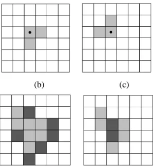
Fig. 1 shows an example of dilation and erosion. The shaded section (defined as A) in Fig. 1(a) represents the “foreground pixels,” and the remainder represents the “background pixels.” The shaded section in Fig. 1(b) is the structuring element, B. The shaded section in Fig. 1(c) is the mapping of structuring element B. Fig. 1(d) is the result after B dilation A. It can be easily seen that dilation makes A larger and the dark parts in Fig. 1(d) comprise the expanded pixels relative to A. Fig. 1(e) is the result after B erosion A. Erosion shrinks A and the dark part comprises the remaining pixels relative to A [46]. Dilation expands an image and erosion shrinks it [47].

(a)

(b) (c)

(d) (e)

Fig. 1. Example of the dilation and erosion processes

Dilation is used to fill holes in an image and the small concave parts of the image edge. Erosion can remove areas that are smaller than the structuring element from the image. If there is a tiny connection between two objects, we can separate them via erosion when the structuring element is sufficiently large [48].

3 Proposed dilation and erosion clustering algorithm

Cluster analysis divides the sample sets into several clusters based on a similarity measure. The samples in the same cluster are as similar as possible, whereas the samples in different clusters are as dissimilar as possible. In general, the smaller the distance of two groups of data, the greater the degree of similarity. Thus, datasets with a small distance should be classified into the same cluster.

When a binary image is imported into MATLAB, it is displayed as a two-dimensional binary matrix that only contains 0 (white) and 1 (black). Therefore, we can transform the original dataset into a binary matrix and perform dilation and erosion on it to form a cluster. Based on the idea above, a new clustering algorithm, called the dilation and erosion (DE) clustering algorithm, is presented. 3.1 Two-dimensional dataset clustering

When an unclassified dataset comprises n groups of two-dimensional (2D) data, we convert the two data of each group into two positive integers, and then use them to set up a 2D matrix. Consequently, each group containing two positive integers can correspond to a point in the specified 2D matrix. Setting the value of these points in the 2D matrix equal to “1” and the others equal to “0,” a 2D binary matrix containing the original data information, called A, is obtained. This matrix only includes “0” and “1”. By dilating A with a 2D circular structuring element B, a new 2D binary matrix, A1, can be generated. Connecting nearby points with value “1” in A1, removing very small areas and separating the tiny connected areas by eroding A1 with a new structuring element C (whose radius is larger than B by “1”), results in the generation of a new 2D binary matrix, A2. Subsequently, some connected areas, which are separated from each other, can be obtained by removing the relatively small connected areas from A2. Moreover, the number of clusters is equal to the number of

4

Next, the groups of data corresponding to the points with value “1” in each connected area are extracted and placed into one cluster. The mean value of the data in each cluster is then defined as the clustering center. Subsequently, the original dataset can be classified into corresponding clusters according to the Euclidean distance between each element and the clustering centers.

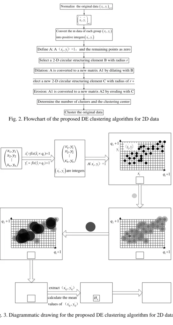
The specific steps used in the DE clustering algorithm are as follows (see Fig. 2):

(1) Normalize all of the original data. There are n groups of data（xi , yi），i = 1, 2, 3, …, n, in the original dataset. Normalize all the data using Eq. (1):

min min

max min max min

ˆ= i ,ˆ i i i x x y y x y x x y y − ₌ − − − (1)

(2) Process the data using Eq. (2):

1 2

ˆ

ˆ

=

(

)+1, y

(

) 1

i i i i

x fix x

′

×

q

′

=

fix y

× +

q

where fix is the truncated integral function, andqj (j=1,2) are suitable integers according to the range of the original dataset.

(3) Obtain the 2D binary matrix. Define A as a （q₁+1）∗（q₂+1） matrix. For matrix A,

' ' , i i

A x y（ ）=1，

i=1,2,3, …, n, and the remaining points are zero. Therefore, A is a 2D binary matrix containing

only ones and zeros.

(4) Perform dilation. Select a 2D circular structuring element B with radius r. Matrix A is converted to a new matrix A1 by dilating with B.

(5) Perform erosion. Set a new 2D circular structuring element C whose radius is 1+r. Matrix A1 is converted to a new matrix A2 by eroding with C.

(6) Determine the number of clusters, k. Display A2 as a binary image in MATLAB, the number of relatively large connected areas in the image is the number of clusters. The number of clusters can also be obtained by removing the relatively small connected areas from A2.

(7) Determine the clustering center,

H

' ' , kj kj

x y

（ ） corresponding to

points with value “1” in each remaining area in A2 and place them in one cluster. The clustering centers are the mean values of the data in these clusters.

(8) Cluster the original dataset. Classify every group data of the original dataset according to the Euclidean distance between itself and clustering centers,

H

2 , i i n x y∧ ∧ ∗       ( ) ( )' '

Convert the m data of each group , into positive integers ,

i i i i

x y x y

( ) 2

Normalize the original data x yi, i n∗

' '

Define A: A（x y_i, _i）=1，and the remaining points as zero

Select a 2-D circular structuring element B with radius r

Dilation: A is converted to a new matrix A1 by dilating with B

Erosion: A1 is converted to a new matrix A2 by eroding with C elect a new 2-D circular structuring element C with radius of r+

Determine the number of clusters and the clustering center

Cluster the original data

Fig. 2.Flowchart of the proposed DE clustering algorithm for 2D data

� �1,�1 �2,�2 ⋮ ��,�� � � �1 , ,�₁, �2 ,_,� 2 , ⋮ ��,,��, �

( )

calculate the mean values of （xkj,ykj）

k

H

6

3.2 m-dimensional dataset clustering

When the unclassified dataset comprises n groups of m-dimensional data, we also can convert the data in each group into positive integers, and then use them to set up an m-dimensional (m-D) matrix. Each set of group data contains m positive integers corresponding to a point in the specified m-D matrix. Setting the value of these points equal to “1” in the m-D matrix and the others equal to “0,” an m-D binary matrix A containing the original data information is constructed with entries “0” or “1.” By dilating A with an m-D structuring element B, a new m-D binary matrix A1 is generated. Then, a new m-D binary matrix A2 is built by eroding A1 with a new structuring element C, whose radius is larger than B by “1.” Subsequently, in accordance with the steps in Section 2.1, the original dataset is clustered.

3.3 Experimental evaluation of the DE clustering algorithm on the UCI datasets

In this section, the feasibility and the performance of the proposed DE clustering algorithm are demonstrated on three different UCI datasets. The details of these datasets are given in Table 1. In the table, it can be seen that different datasets have different dimensions. The algorithm was tested using MATLAB.

Table 1 Details of the UCI datasets

Datasets Number

of samples

Dimensions True number of

clusters Far_4k2 Haberman Iris 400 306 150 2 3 4 4 2 3

Because of the different spatial distributions and sample sizes of these datasets, we chose different parameters for the different datasets. The selected parameters of the three datasets are shown in Table 2.

Table 2 Parameters of the UCI datasets

Datasets qi Radius r of B Far_4k2 Haberman Iris q1=q2=200 q1=q2=50, q3=30 q1=q4=30, q2=25, q3=20 7 6 3

The mean value of two dimensions for the Far_4k2 datasets are 5.364 and 5.4836. As they are approximately equal to each other, we chose q1=q2=200. Based on the fact that the mean value of three dimensions for the Haberman datasets are 52.45, 62.85, and 4.03, we set q1=q2=50 and q3=30.

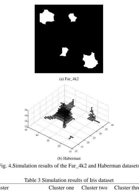
The simulation results are shown in Fig. 4. The Far_4k2 datasets can be divided into four clusters, and the Haberman datasets can be divided into two clusters. The Iris dataset can be divided into three clusters, as shown in Table 3. These numbers of the clusters are completely consistent with the true numbers of clusters in Table 1. As the number of dimension of the Iris dataset is four (greater than three), its classification result is difficult to display graphically.

(a) Far_4k2 10 15 20 25 30 35 40 10 20 30 40 50 12 14 16 18 (b) Haberman

Fig. 4.Simulation results of the Far_4k2 and Haberman datasets Table 3 Simulation results of Iris dataset

Cluster Cluster one Cluster two Cluster three

Number of samples in each cluster

4739 19410 759

4 Wind power prediction and results analysis

4.1 Wind power prediction model

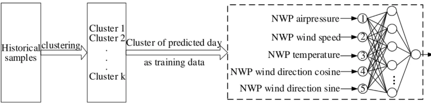
Wind power generation fluctuates with weather conditions, particularly wind speed and direction. Dong et al. [26] showed that the days with similar wind power variation trends also have similar meteorological phenomena. Therefore, the historical days with similar NWP meteorological information were classified into one cluster by the DE clustering algorithm, and the data in the cluster to which the prediction day belongs were selected as the training samples. Then, the generalized regression neural network (GRNN) model was established, with the NWP information as input and wind power as output. The NWP information includes air pressure, wind speed, temperature, and sine and cosine values of wind direction. The NWP information of the predicted day is sent to the trained model to obtain the wind power prediction. The wind power prediction method based on cluster analysis is shown in Fig. 5.

8 Historical samples Cluster 1 Cluster 2 . . . Cluster k clustering 1 2 3 NWP airpressure NWP wind speed NWP temperature Wind power .. .

NWP wind direction cosine NWP wind direction sine

4 5 Cluster of predicted day

as training data

Fig. 5. Wind power prediction method based on cluster analysis

Therefore, there are three steps in the wind power generation prediction: clustering with three different algorithms to extract the training data; and then building power prediction model by GRNN using the selected training data; finally, wind power prediction using the GRNN model. GRNN model here can be replace by any other models in the field of wind power prediction.

In this section, we classify the NWP information of the historical days with three different clustering algorithms respectively and compare the prediction results from actual wind farm. The prediction results are based on the three different clustering algorithms of the same prediction model. The three different clustering algorithms are the proposed DE clustering algorithm, and two existing commonly used clustering algorithms—the DPK-medoids clustering algorithm and the K-means clustering algorithm.

4.2 Database description

Data from January 2012 to June 2012 of Yilan wind farm in Heilongjiang Province, in the northeast of China, including the wind power from the wind farm and the NWP data from the high-resolution atmospheric model of ECMWF (ECMWF- HRES) [49], were used for analysis, modeling, and prediction in this case study.

The longitude and latitude coordinates of Yilan wind farm are, east longitude 129.71°-129.73° and north latitude 46.23°-46.57°. The map of the location of Yilan wind farm in Heilongjiang Province, Fig.16, is attached in Appendix as a reference. The wind power used in this case study is from the first stage of the wind farm (Ⅰ), which has 33 wind turbines (each 1.5MW). The wind power of the whole wind farm with a temporal resolution of 15 min was collected from the Supervisory Control and Data Acquisition (SCADA) system. The temporal resolution of the NWP data from ECMWF was 1h. In order to meet the requirement of the State Grid of China, it was interpolated to 15min temporal resolution before the modeling in this case study.

There are two stages in the modeling: clustering to select the training data, building power prediction model by the selected training data. After the modeling, June 30, 2012, was chosen to evaluate the performance of the different prediction models. That is, the final input and output of the completed prediction model are the NWP data of June 30, 2012 and the corresponding wind power prediction values, which will be compared with the actual power. So June 30, 2012 is named the predicted day.

In clustering stage, all of the weather data, from January 01, 2012 to June 30, 2012, is used to identify the cluster which the predicted day (June 30, 2012) belongs to.

NWP information of every day can be seen as a data object that is expressed as an eight-dimensional vector X=[Pav, Vmin, Vmax, Tmin, Tmax, Dsin, Dcos, Vmean], called the daily NWP vector. The respective meaning of the eight components is as follows: daily average air pressure, daily minimum wind speed, daily maximum wind speed, daily minimum temperature, daily maximum

temperature, daily average wind direction sine value, daily average wind direction cosine value, and daily mean wind speed. Every component of the NWP daily vector needs to be normalized. To do this air pressure, wind speed, and temperatures are divided by the maximum value in history.

To reduce the amount of calculation, we selected three components from vector X for clustering. Meanwhile, because the goal of meteorological data classification is to improve the prediction accuracy of wind power, the three most relevant components were chosen after comparing the relevance of the eight components and wind power, respectively. Finally, Vmin, Vmax, and Vmean were selected for clustering.

After the clustering, the days whose NWP information is similar to the predicted day are chosen and forwarded to train the prediction model.

The Train and Test Datasets of the prediction model are illustrated below:

Train Datasets: the NWP and power information of the days chosen from the clustering above, including wind speed, sine of wind direction, cosine of wind direction, temperature, air pressure, power. The temporal resolution is 15min.

Test Datasets: the NWP and power information of June 30, 2012, including wind speed, sine of wind direction, cosine of wind direction, temperature, air pressure, power. The power here is used to evaluate the performance of the data mining method. The temporal resolution is 15min.

Timescale of prediction: 1 day. Prediction steps: 96.

4.3 Clustering and simulation results

Firstly, we classify the NWP information of the historical days with three different clustering algorithms respectively for the predicted day. And then, different clustering results are compared and analyzed.

4.3.1 The DE clustering algorithm

According to the DE clustering algorithm in Section 2, the DE clustering procedure includes the following steps:

(1) Normalize all the original data. There are 182 groups of data（x_i,y ,_i z_i），i=1,2,3,…,182, in the original dataset. Normalize all the data according to Eq. (1).

(2) Process the data using Eq. (2) and setting the parameters q1=40, q2=60, q3=50.

(3) Obtain the 2D binary matrix. Define A as a 41 61 51∗ ∗ matrix. For matrix A, A（x′ ′_i,y ,_i z_i'）=1，

i=1,2,3,…, n, and the remaining points are zero. Therefore, A is a 3D binary matrix containing

only ones and zeros.

(4) Dilation. Select a 3D circular structuring element B with radius

r

=4

(5) Erosion. Set a new 3D circular structuring element C with radius

r

=4

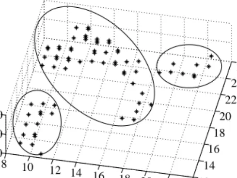
(6) Determine the number of clusters. When A2 displayed as a binary image in MATLAB, the number of relatively large connected areas in the image is the number of clusters. The clustering result is shown in Fig. 6.

10 8 ₁₀ 12 14 16 _{18 20 22} 2412 14 16 18 20 22 24 26 10 20 30

Fig. 6. Clustering result

(7) Determine the clustering center and cluster the original dataset. Calculate the mean of each cluster as its clustering center and classify the 182 historical days according to the Euclidean distance between itself and the clustering centers. Then, the historical days are divided into three clusters: the first cluster consists of 78 days, the second cluster has 39 days, and the third cluster has 65 days. The predicted day belongs to the second cluster.

4.3.2 The DPK-medoids clustering algorithm

Xie et al. [40] proposed the DPK-medoids clustering algorithm. The algorithm defines the local density ρ_iof point xi as the reciprocal of the sum of the distance between xi and its t nearest neighbors. The new distanceδ_iof point xi is defined as well, and then the decision graph of a point distance relative to its local density is plotted. The points with higher local density and apart from each other located at the upper right corner of the decision graph, which are far away from the remaining points in the same dataset, are chosen as the initial seeds for K-medoids, such that the seeds will be in different clusters and the number of clusters of the dataset is automatically determined as the number of initial seeds.

Following classification of the 182 historical days based on the DPK-medoids clustering algorithm, the result shown in Fig. 7 was obtained. The number of clusters can either be three or four. The details are as follows.

Local density D is ta n c e 0 0.2 0.4 0.6 0.8 1 1.2 1.4 1.6 1.8 2 1 1.5 2 2.5 Curve1 Curve 2

Fig. 7. The decision graph

142th day, representing three clustering centers. The 182 historical days are divided into three clusters with the first cluster comprising 95 days, the second cluster 39 days, and the third cluster 48 days. The predicted day belongs to the third cluster.

Four clusters: In the upper right corner of curve 2 in Fig. 7, there are four points, 9th _{day, 70}th _day,

105th day, and 142nd day, representing four clustering centers. The 182 historical days are divided into four clusters, with the first cluster comprising 50 days, the second cluster 45 days, the third cluster 39 days, and the fourth cluster 48 days. The predicted day belongs to the fourth cluster.

4.3.3 The K-means clustering algorithm

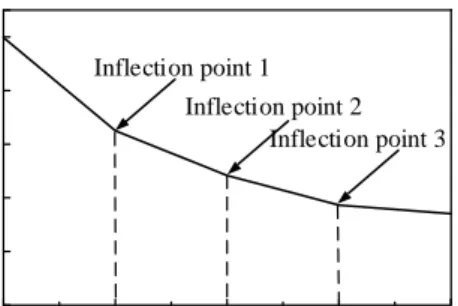
The K-means clustering algorithm [26, 50, 51] is one of the most classic dynamic clustering algorithms. Its basic idea is to divide each sample into the nearest category, which is then clustered according to the distance. It uses the nearest neighbor rule, the squared error sum, as a criterion function. The value of this criterion function changes with the cluster k. The optimal number of clusters is determined by the inflection point of the curve, which is the relation of the criterion function and the number of clusters, k. Fig. 8 shows the result of classification of the 182 historical days using the k-means cluster algorithm.

2 3 4 5 6 0.0 0.4 0.8 1.2 1.6 2.0 Cri te ri on func ti on K Inflection point 1 Inflection point 2 Inflection point 3

Fig. 8. Relationship between the criterion function and the number of clusters, k

The degree of turning at the inflection point k=3 is not obvious; therefore, k=4 and k=5 are also selected as the number of clusters to avoid erroneous judgment.

When the number of clusters k=3, the first cluster comprises 88 days, the second cluster 57 days, and the third cluster 37 days. The predicted day belongs to the second cluster.

When the number of clusters k=4, the first cluster comprises 75 days, the second cluster 26 days, the third cluster 37 days, and the fourth cluster 44 days. The predicted day belongs to the fourth cluster.

When the number of clusters k=5, the first cluster comprises 41 days, the second cluster 24 days, the third cluster 22 days, the fourth cluster 37 days, and the fifth cluster 58 days. The predicted day belongs to the fourth cluster.

4.3.4 Analysis of the different clustering algorithms

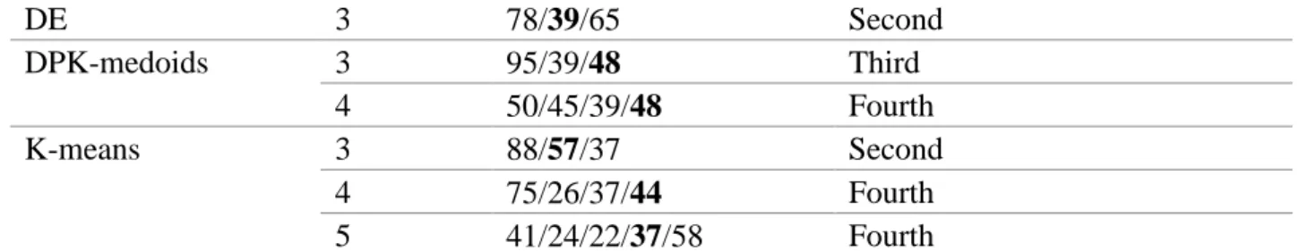
The clustering results from the different algorithms are shown in Table 4. As can be seen, the number of clusters of the DPK-medoids clustering algorithm and the K-means clustering algorithm are uncertain and need artificial participation. In contrast, the proposed DE clustering algorithm does not need the number of clusters to be specified beforehand, and clustering is automatically carried out without manual involvement.

12

Clustering algorithm Number of clusters

Number of samples in each cluster

Cluster to which the predicted day belongs DE 3 78/39/65 Second DPK-medoids 3 95/39/48 Third 4 50/45/39/48 Fourth K-means 3 88/57/37 Second 4 75/26/37/44 Fourth 5 41/24/22/37/58 Fourth

4.4 Wind prediction results analysis

4.4.1 Performance of the different clustering algorithms in wind power prediction

Based on the clustering algorithms above, the data about the cluster to which the predicted day belongs was selected and applied to train a GRNN model. The number of samples in the predicted dataset was 96. There were six classifications from the three clustering algorithms above to be used to predict the predicted day’s wind power generation, respectively.

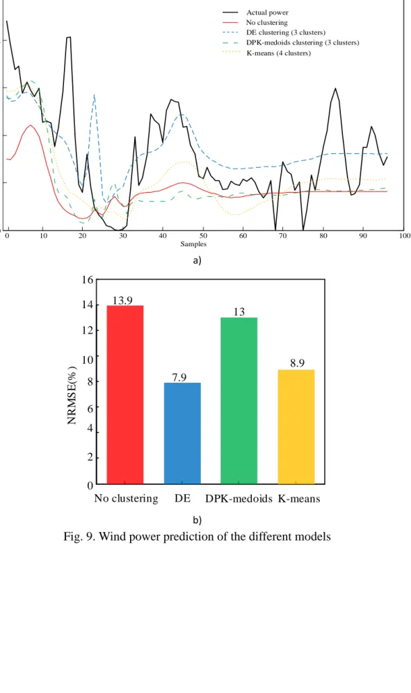
The GRNN without the clustering prediction model, which was trained using all the historical samples, was considered as the reference model. Compared with this reference model, the model training time is much faster after clustering, which is about 1.2s, and the time of the reference model is about 7.7s. Table 5 shows the normalized root mean squared error (NRMSE) of all the prediction results. The prediction results of these prediction models are intuitively shown in Fig. 9, and the prediction errors are depicted in Fig.10.

Table 5 Prediction errors of the different models

Prediction model Number

of clusters NRMSE (%) GRNN without clustering 1 13.9 DE clustering-GRNN 3 7.9 DPK-medoids clustering-GRNN 3 13.0 4 13.0 K-means clustering-GRNN 3 13.7 4 8.9 5 9.2

0 10 20 30 40 50 60 70 80 90 100 0 0.5 1 1.5 2 2.5 x 104 P o w er (kW ) Actual power Samples No clustering DE clustering (3 clusters) DPK-medoids clustering (3 clusters) K-means (4 clusters)

a)

No clustering DE DPK-medoids K-means 0 2 4 6 8 10 12 14 16 N R MS E (% ) 13.9 7.9 13 8.9 b)

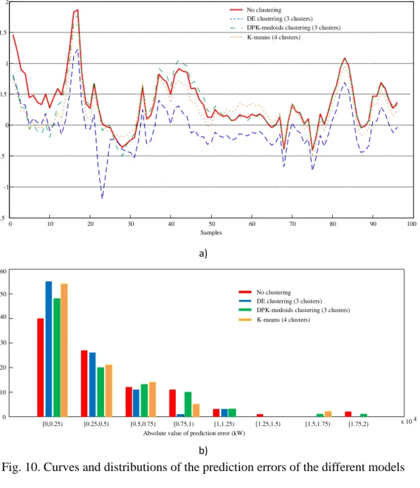
14 0 10 20 30 40 50 60 70 80 90 100 -1.5 -1 -0.5 0 0.5 1 1.5 2 x 10 4 P re di ct ion e rr or s (kW ) Samples No clustering DE clustering (3 clusters) DPK-medoids clustering (3 clusters) K-means (4 clusters)

a)

Absolute value of prediction error (kW)

No clustering DE clustering (3 clusters) DPK-medoids clustering (3 clusters) K-means (4 clusters) [0,0.25) 0 10 20 30 40 50 60 x 10 4 [0.25,0.5) [0.5,0.75) [0.75,1) [1,1.25) [1.25,1.5) [1.5,1.75) [1.75,2) N um be r b)

Fig. 10. Curves and distributions of the prediction errors of the different models Table 6 Percentages with the minimal prediction error of the different models

Prediction model Number

of clusters

percentages with the minimal error (%)

GRNN without clustering 1 14.6

DE clustering-GRNN 3 47.9

DPK-medoids clustering-GRNN 3 11.5

K-means clustering-GRNN 4 26.0

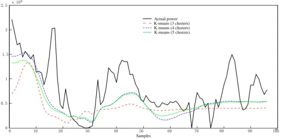
For the K-means based models, there are three different NRMSEs in Table 5 because of the different classifications. For further explanation, the corresponding three prediction curves are shown in Fig. 11.

Actual power K-means (4 clusters) K-means (5 clusters) K-means (3 clusters) 0 10 20 30 40 50 60 70 80 90 100 0 0.5 1 1.5 2 2.5 x 104 Samples P re di c ti on e rr or s (kW )

Fig. 11. Wind power prediction of the K-means clustering algorithm The following deductions can be made from the Table 5-6 and Figs.9-11 above:

(1) Whether from NRMSE or from the error distribution, it can be seen that the prediction performance from the GRNN without clustering model is the worst. GRNN without clustering model can only predict the trend of the power, but not reflect the volatility of the power. The NRMSE of This is because that the training data of this model is all the historical samples. There is a large amount of information low related to the predicted day, which increases the generalization ability of the model and reduces the learning ability for special situation. Besides, it is worth mentioning that this large amount of training data not only does not improve the prediction accuracy, but also greatly slows down the training speed of the model.

Therefore, it is clear that clustering of the training samples is necessary.

(2) Table 5 and Fig. 9 b) show that the proposed DE clustering-GRNN model generates the lowest NRMSE among the six prediction models based on the clustering algorithm. Moreover, the DE clustering-GRNN model exhibits the best prediction capability not only based on the NRMSE value but also on the prediction curves in Figs. 9. When the prediction model is the proposed DE clustering-GRNN model, the prediction curve is close to the actual curve.

(3) Based on the prediction error curves in Fig.10 a), it can be seen that the errors from DE clustering-GRNN model is minimal most of the time. The percentages with the minimal error are showed in Table 6. The percentage with the minimal error of DE clustering-GRNN model is 47.9%, which is much larger than the other three percentages.

At the same time, Fig.10 b) gives the distributions of prediction errors. It can be observed that the prediction errors from DE clustering-GRNN model are distributed within a small error range, [0, 1.25). Moreover, the number in the minimum prediction error interval from this model is 55, which is the biggest compared to the other three models.

(4) For the K-means based models, the prediction results depend on the selection of k. The NRMSE in Table 5 and the prediction curve in Fig. 11 indicate that when k = 4, the prediction performance is best.

4.4.2 Comparison with AM for wind power prediction

Because the DE clustering algorithm presented in this paper is based on the meteorological similarity, an Analogue Method (AM) based prediction model, called AM-GRNN, was used here to

16

The AM is based on the principle that two similar states of the atmosphere lead to similar local effects. Thus, the AM consists of searching for a certain number of past situations in meteorological data, in such a way that they present similar properties to that of a target situation for any chosen variables [52]. Many AM techniques exist and have been compared in detail in the literature, with a wide range of energy-related applications [23, 53, 25]. In the present analysis, the traditional AM was used to extract the historical days whose NWP information is similar to that of the predicted day as training samples of the GRNN model. These historical days can be called “analogs” in AM algorithm.

The metric in the traditional AM used to rank the quality of an analog is defined as follows [23, 53]:

�|�_�,�_�|�= ∑ ��

�_���∑�̃_�=−�̃(��,�+� − ��,�+�)2

��

�=1 (3)

Where �_� is the current NWP forecast for the time step � at a certain location, �_� is an analog forecast for the time step � of the training period (� corresponding to the same time steps as � but on a different day) and at the a certain location, �_� and �_� are the number of physical variables and their weights, respectively, �_�� is the number of standard deviation of the time series of the historical forecasts of a given variable, �̃ is an integer equal to half with of the time window over which the metric is compute, and �_�,�+� and �_�,�+�are the values of the analog and the forecast in the time window for given variable.

The goal of AM here is to find n historical days (analogs) of the NWP variables (chosen among the NWP with the highest correlation with the wind power, Vmin, Vmax, and Vmean in this case study) that were similar with that of the predicted day. Therefore, �_� = 1 and �̃= 0 in Eq. (3). The weight � is calculated by the correlation coefficient with the wind power:

� = [0.715, 0.807, 0.938] (4) After obtaining the n analogs by calculating Eq. (3), the NWP information data in the analogs were selected as the training samples of the GRNN model. The wind power prediction method based on traditional AM (AM-GRNN model) is shown in Fig. 12. The number of analogs n is a parameter need to calibrate [23, 25]. In the present analysis, n is set based on the criterion function NRMSE. The NRMSE values are computed with different n from 1 to 60, shown in Fig.13. It is shown that NRMSE decreases with increasing n at the beginning, tends to be stable value after n=25. Therefore,

n=25 is chosen as the optimal value to obtain the best analogs and prediction for AM-GRNN model,

which is used to compare with the proposed DE clustering-GRNN model.

Historical samples Analog 1 Analog 2 . . . Analog n AM 1 2 3 NWP airpressure NWP wind speed

NWP temperature Wind _power

.. .

NWP wind direction cosine NWP wind direction sine

4 5

n historical days

(analogs) as training data

0 10 20 30 40 50 60 8 10 12 14 16 18 20

The number of analogs n

NR M S E ( %)

Fig. 13. The NRMSE values from n=1 to n=60

Table 7 shows the NRMSEs from the proposed DE clustering-GRNN and AM-GRNN. The prediction results of these prediction models are shown in Fig. 14, and the prediction errors are depicted in Fig.15.

Table 7 Prediction errors of DE clustering-GRNN and AM-GRNN

Prediction model NRMSE (%)

DE clustering-GRNN 7.9 AM-GRNN 9.7 0 10 20 30 40 50 60 70 80 90 100 0 0.5 1 1.5 2 2.5 x 10 4 P re di ct ion e rr or s (kW ) Samples Actual power DE clustering ( NRMSE=7.9) AM (NRMSE=9.7)

18 x 104 0 10 20 30 40 50 60 70 80 90 100 -1.5 -1 -0.5 0 0.5 1 1.5 DE clustering ( NRMSE=7.9) AM (NRMSE=9.7) P re di ct ion e rr or s (kW ) Samples 0 10 20 30 40 50 60 N um be r

Absolute value of prediction error (kW)

[0,0.25) [0.25,0.5) [0.5,0.75) [0.75,1) [1,1.25) [1.25,1.5) x 10 4 DE clustering ( NRMSE=7.9)

AM (NRMSE=9.7)

a) b)

Fig. 15. Curves and distributions of the prediction errors of DE clustering-GRNN and AM-GRNN Table 7 and Fig.14 show that, compared with AM-GRNN model, the proposed DE clustering-GRNN model exhibits the better prediction capability. And based on the prediction error curves in Fig.15, it can be seen that the prediction errors from DE clustering-GRNN model are distributed within a smaller error range [0, 1.25), while that of AM-GRNN model is [0, 1.5). And, the number in the minimum prediction error interval from DE clustering-GRNN model is 55, while this number of AM-GRNN model is only 46.

In addition to these prediction performances compared to the proposed DE clustering-GRNN model, the AM-GRNN model cannot automatically predict because some parameters in Eq. (3) cannot be chosen automatically [25], such as the number of analogs n in the present analysis. This number is likely dependent on the length of the training period and the available analog predictors, and cannot be generalized for other data sets [23]. In this paper, the value of n is set to 25 based on the criterion function NRMSE, but obviously it does not necessarily apply to other different applications. For the new application, the value of n needs to be re-selected according to the new data set or the new criterion. This operation is not adaptive and increases the workload and time of the modeling.

4.4.3 Evaluation of the predictions

In summary, the comparison and statistical test results reveal the following:

(1) Using the correct clustering algorithm to choose the historical days whose NWP information is similar to the predicted day as the model training samples can improve the prediction accuracy. (2) Existing clustering algorithms, especially the K-means clustering algorithm, cannot guarantee a

unique and optimal prediction because of their dependence on the artificial selection of k.

(3) There are some shortcomings of the traditional AM when it is used for wind power prediction. For instance, the prediction model based on traditional AM is not adaptive and cannot predict automatically.

(4) The proposed DE clustering-GRNN model gives the best performance among the prediction models used in this paper, not only because of the high prediction accuracy, but also because it can cluster automatically without supervision, and its k does not need to be specified in advance. 5 Conclusions

clustering algorithm, which has its foundation in mathematical morphology. The proposed model first classifies the historical days with similar NWP meteorological information into the same cluster based on the DE clustering algorithms. Then, samples of the cluster to which the predicted day belongs are used to train the GRNN, which is then used to predict the wind power. The feasibility of the proposed model was verified using numerical weather prediction (NWP) data and actual wind power data from a wind farm.

Compared to the GRNN without the clustering prediction model, the prediction results show that the GRNN with a suitable cluster method is more effective in terms of the improving accuracy of day-ahead wind power prediction, and can reduce the training time of modeling. In order to verify and compare the prediction performance of the proposed DE clustering-GRNN model, some prediction models based on existing algorithms—DPK-medoids clustering-GRNN, and K-means clustering-GRNN—were used with the same sample data. And, AM-GRNN model, which is based on the traditional AM algorithm, was also be applied in the case study to evaluate the proposed DE clustering-GRNN.

According to the comparison results, it can be observed that: 1) in the clustering stage, the proposed DE clustering algorithm can effectively cluster the NWP data; 2) in the prediction stage, the proposed DE clustering-GRNN model can have a good prediction accuracy. Therefore, the new proposed DE clustering-GRNN model is suitable in the field of day-ahead wind power prediction.

A major advantage of the DE clustering algorithm is that it does not need the number of clusters to be specified beforehand and it can perform clustering automatically without external supervision. These excellent qualities make the output of this clustering algorithm unique and optimal, and the prediction model based on this clustering algorithm adaptive.

In fact, converting the dataset to a binary matrix is not the only way of data processing in the DE clustering algorithm. As future work, we plan to convert the dataset to a greyscale matrix and cluster the dataset according to the gray boundary. Besides, it would be useful to discuss the prediction errors when the weather pattern is different for getting more information of the relationship between the wind power and the meteorological data. Hence, as a continuation, we can do more research with more innovative data analysis and data mining techniques.

Conflicts of interest

The authors declare that there are no conflicts of interest regarding the publication of this paper. Acknowledgment

Funding: This work was supported by the Natural Science Foundation of China [grant number 51607009].

Appendix

Data from January 2012 to June 2012 of Yilan wind farm in Heilongjiang Province, in the northeast of China, were used in this case study. The longitude and latitude coordinates of Yilan wind farm are, east longitude 129.71°-129.73° and north latitude 46.23°-46.57°. Fig.16 is the map of the location of Yilan wind farm in Heilongjiang Province. The wind power used in this case study is from the first stage of the wind farm (Ⅰ), which has 33 wind turbines (each 1.5MW).

20 Harbin

Yilan Russsia

Yilan wind farm (I, 33 wind turbines)

100 km

Heilongjiang Province Inner Mongolia

Province

Jilin province

Fig. 16. The map of the location of Yilan wind farm in Heilongjiang Province References

[1] Yuan X, Chen C, Yuan Y, Huang Y, Tan Q. Short-term wind power prediction based on LSSVM-GSA model. Energy Conversion and Management 2015; 101: 393-401.

[2] Exizidis L, Kazempour SJ, Pinson P, de Greve Z, Vallée F. Sharing wind power forecasts in electricity markets: A numerical analysis. Applied Energy 2016; 176: 65-73.

[3] Higgins P, Foley AM, Dougla R, Li K. Impact of offshore wind power forecast error in a carbon constraint electricity market. Energy 2014; 76: 187-197.

[4] Zhao J, Guo Y, Xiao X, Wang J, Chi D, Guo Z. Multi-step wind speed and power forecasts based on a WRF simulation and an optimized association method. Applied Energy 2017; 197: 183-202. [5] Skittides C, Früh WG. Wind forecasting using principal component analysis. Renew Energy 2014;

69: 365-74.

[6] Douak F, Melgani F, Benoudjit N. Kernel ridge regression with active learning for wind speed prediction. Applied Energy 2013; 103: 328-40.

[7] Yesilbudak M, Sagiroglu S, Colak I. A new approach to very short term wind speed prediction using k-nearest neighbor classification. Energy Conversion Management 2013; 69: 77-86.

[8] De Giorgi MG, Ficarella A, Tarantino M. Assessment of the benefits of numerical weather predictions in wind power forecasting based on statistical methods. Energy 2011; 36: 3968-3978. [9] Masseran N. Markov Chain model for the stochastic behaviors of wind direction data. Energy

Conversion Management 2015; 92: 266-274

[10] Chen K, Yu J. Short-term wind speed prediction using an unscented Kalman filter based state-space support vector regression approach. Applied Energy 2014; 113: 690–705.

[11] Liu H, Tian HQ, Li YF. Comparison of two new ARIMA-ANN and ARIMA-Kalman hybrid methods for wind speed prediction. Applied Energy 2012; 98: 415-24.

[12] Su Z, Wang J, Lu H, Zhao G. A new hybrid model optimized by an intelligent optimization algorithm for wind speed forecasting. Energy Conversion Management 2014; 85: 443-52.

[13] Chitsaz H, Amjady N, Zareipour H. Wind power forecast using wavelet neural network trained by improved Clonal selection algorithm. Energy Conversion Management 2015; 89: 588-98. [14] Liu H, Tian HQ, Li YF, Zhang L. Comparison of four AdaBoost algorithm based artificial

neural networks in wind speed predictions. Energy Conversion Management 2015; 92: 67-81. [15] Peng H, Liu F, Yang X. A hybrid strategy of short term wind power prediction. Renew Energy

2013; 50: 590-595.

[16] De Giorgi MG, Ficarella A, Tarantino M. Assessment of the benefits of numerical weather predictions in wind power forecasting based on statistical methods. Energy 2011;36:3968-78. [17] Zhao Y, Ye L, Li Z, Song X, Lang Y, Su J. A novel bidirectional mechanism based on time

series model for wind power forecasting. Applied Energy 2016; 177: 793-803.

[18] Li G, Shi J. On comparing three artificial neural networks for wind speed forecasting. Applied Energy 2010; 87: 2313-20.

[19] Liu H, Tian HQ, Pan DF, Li YF. Forecasting models for wind speed using wavelet, wavelet packet, time series and artificial neural networks. Applied Energy 2013; 107: 191–208.

[20] Zhao W, Wei YM, Su Z. One day ahead wind speed forecasting: A resampling based approach. Applied Energy 2016; 178: 886–901.

[21] Liu H, Tian HQ, Liang XF, Li YF. Wind speed forecasting approach using secondary decomposition algorithm and Elman neural networks. Applied Energy 2015; 157: 183–94.

[22] Yesilbudak M, Sagiroglu S, Colak I. A novel implementation of kNN classifier based on multi-tupled meteorological input data for wind power prediction. Energy Conversion Management 2017; 135: 434-444.

[23] Vanvyve E, Delle Monache L, Monaghan AJ, and Pinto JO. Wind resource estimates with an analog ensemble approach. Renewable Energy 2015; 74,: 761–773.

[24] Horton P, Jaboyedoff M, Metzger R, Obled C, and Marty R. Spatial relationship between the atmospheric circulation and the precipitation measured in the western Swiss Alps by means of the analogue method. Natural Hazards and Earth System Sciences 2012; 12,: 777–784.

[25] Horton P, Jaboyedoff M, Obled C. Using genetic algorithms to optimize the analogue method for precipitation prediction in the Swiss Alps. Journal of Hydrology 2018; 556: 1220-1231. [26]Dong L, Wang LJ, Khahro SF, Gao S, Liao XZH. Wind power day-ahead prediction with cluster

analysis of NWP. Renewable and Sustainable Energy Reviews 2016; 60: 1206-1212.

[27] Azimi R, Ghofrani M, Ghayekhloo M. A hybrid wind power forecasting model based on data mining and wavelets analysis. Energy Conversion and Management 2016; 127: 208-225

[28] Erilli NA, Yolcu U, Eğrioğlu E, Aladağ ÇH, Öner Y. Determining the most proper number of cluster in fuzzy clustering by using artificial neural networks. Expert Systems with Applications 2011; 38(3): 2248-2252.

[29] Rhodes JD, Cole WJ, Upshaw CR, Edgar TF, Webber ME. Clustering analysis of residential electricity demand profiles. Applied Energy 2014; 135: 461-471.

[30] Yu S, Wei YM, Fan J, Zhang X, Wang K. Exploring the regional characteristics of inter-provincial CO2 emissions in China: An improved fuzzy clustering analysis based on particle swarm optimization. Applied Energy 2012; 92: 552-562.

[31] Zhou T, Lu HL. Clustering algorithm research advances on data mining. Computer Engineering and Application 2012; 48(12):100-111.

[32] McLoughlin F, Duffy A, Conlon M. A clustering approach to domestic electricity load profile characterisation using smart metering data. Applied Energy 2015; 141: 190-199.

[33] Guan X, Qian Y, Sun X. An improved clustering algorithm based on local density. Telecommunications Science 2016; 32(1): 54-59.

[34] Mena R, Hennebel M, Li YF, Zio E. Self-adaptable hierarchical clustering analysis and differential evolution for optimal integration of renewable distributed generation. Applied Energy

22

[35] Zhou SB, Xu ZY, Tang XQ. New method for determining optimal number of clusters in K-means clustering algorithm. Computer Engineering and Application 2010; 46(16): 27-31

[36] Wei J, Lu J, Peng F. Research on a method of self-adaptation of the number of clusters for hierarchical initialization clustering. Electronic Design Engineering 2015; 23(6): 5-8

[37] Řezanková H, Húsek D. Fuzzy clustering: Determining the number of clusters. Computational

Aspects of Social Networks (ICCASoN), International Conference on IEEE 2012: 277-282 [38] Sun C, Kong W, Dai G. A spectral clustering with ascertainable clustering number. Journal of

Hangzhou Dianzi University 2010; 30(2): 53-56

[39] Zhang Y, Xu X, Ye Y. NSS-AKmeans: An agglomerative fuzzy K-means clustering method with automatic selection of cluster number. Advanced Computer Control (ICACC), International Conference on IEEE 2010; 2: 32-38.

[40] Xie J, Qu Y. K-medoids clustering algorithms with optimized initial seeds by density peaks. Journal of Frontiers of Computer Science and Technology 2016; 10(2): 230-247.

[41] Muneeswaran P, Velvizhy P, Kannan A. Clustering fusion with automatic cluster number. Recent Trends in Information Technology (ICRTIT), International Conference on IEEE 2014: 1-6.

[42] Khabou MA, Gader PD. Erosion and dilation as solutions to regularization problem. International Society for Optics and Photonics 1997: 106-111.

[43] Ruan Q. Digital image processing. Electronic Industry Press; 2001. p. 35.

[44] Cochrane GR, Lafferty KD. Use of acoustic classification of sidescan sonar data for mapping benthic habitat in the Northern Channel Islands, California. Continental Shelf Research 2000; 22(3):112-114.

[45] Agam G. Regulated morphological operations. Pattern Recognition 1999; 32:133-134.

[46] Hua W. Research of image processing algorithm based on mathematic morphology. Harbin: Harbin Engineering University; 2007.

[47] Benoso BL, Nazuno JF, Márquez CY, Yáñez IL. Cellular mathematical morphology. Sixth Mexican International Conference on Artificial Intelligence, Special Session (MICAI). International Conference on IEEE 2007: 105-112.

[48] He D, Geng N, Yi Z. Digital image processing. Xidian University Press; 2003. p. 170-200. [49] Ling J, Bauer P, Bechtold P, Beljaars A, Forbes R, Vitart F, UlateM, Zhang CD. Global versus

Local MJO Forecast Skill of the ECMWF Model during DYNAMO. Monthly Weather Review 2014; 142: 2228-2247.

[50]Al-Shammari ET, Shamshirband S, Petkovic D, Zalnezhad E, Yee PL, Taher RS, Cojbasic Z. Comparative study of clustering methods for wake effect analysis in wind farm. Energy 2016; 95: 573-579.

[51] Li S, Ma H, Lia W. Typical solar radiation year construction using k-means clustering and discrete-time Markov chain. Applied Energy 2017; 205: 720-731.

[52] Salcedo-Sanz S, García-Herrerab R, Camacho-Gómez C, Aybar-Ruíz A, Alexandre E. Wind power field reconstruction from a reduced set of representative measuring points. Applied Energy 2018; 228: 1111-1121.

[53] Alessandrini S, Delle Monache L, Sperati S, Nissen JN. A novel application of an analog ensemble for short-term wind power forecasting. Renewable Energy 2015; 76: 768–78.