Zurich Open Repository and Archive University of Zurich Main Library Strickhofstrasse 39 CH-8057 Zurich www.zora.uzh.ch Year: 2018
Automatic Sleep Classification with Machine Learning
Malafeev, AlexanderAbstract: Sleep is ubiquitous in nature. Humans spend a third of their lives sleeping. And yet, despite all the recent advances in the field, we still don’t know the purpose of sleep. However, sleep disorders are detrimental for health and quality of life and insomnia is one of the most common sleep disorders. Excessive daytime sleepiness or insufficient sleep decreases cognitive performance and may cause accidents. These facts suggest that understanding sleep and its regulation is very important. In the first chapter I summarized the most recent hypotheses on the purpose of sleep; then I described the gold standard of assessing sleep – polysomnography (PSG), sleep stages and particularly the electroencephalogram (EEG). Furthermore, an overview of machine learning tools is provided as they will be used to classify sleep stages and detect microsleep episodes. In the second chapter we implemented and tested 14 simple artifact detection methods and conducted a thorough analysis of their performance on two datasets, one comprised sleep recordings of healthy young subjects, the other one data recorded in patients with hypersomnia and narcolepsy. We found that clean average EEG power density spectra can be obtained using very simple methods. We got the best performance of artifact detection with thresholding slope, power in high frequency (25-90 Hz or 45-90 Hz) and the residual errors of an autoregressive model fitted to the EEG. It is not surprising that the power in high frequency range was a good predictor of an artifact as muscle artifacts are characterized by the power in high frequency range. Most methods showed good sensitivity. However, since we had chosen fixed false positive rate (FPR) of 10%, we excluded on average 16.3% of the epochs whereas experts excluded on average only 7% of the epochs. Our approach seemed reasonable as it leaves enough data for subsequent analyses. The main chapter (third chapter) describes the developed automatic sleep scoring algorithms. Scoring rules are complex and to some degree subjective. Despite the fact that human brain has superb image recognition abilities, sleep scoring is a difficult task. Thus, it is not possible to just program an algorithm which implements the scoring rules for sleep. Such a problem can be addressed however, with modern machine learning methods. Such algorithms learn from the examples which have already been analyzed by an expert. With these techniques we don’t even need to know how to score sleep stages ourselves, we just need examples of experts. We developed several algorithms ranging from basic machine learning tools to deep artificial neural networks. First, we engineered 20 features derived from EEG, EOG and EMG data. This process reduces the dimensionality of our data and makes classification of the data easier. We employed a random forest (RF) classifier in conjunction with a Hidden Markov Model (HMM) or a moving median filter (MF) to smooth the data. Alternatively, we applied artificial neuronal networks (ANN), Long-Short Term Memory (LSTM) networks, designed to handle time series to classify the data. We used our engineered features as input for these networks. Finally, we employed deep convolutional neural networks (CNNs) in combination with LSTM networks. Such algorithms (CNN-LSTM networks) work with raw data and do not require engineered features. We used the F1 score, a performance measure of multi-class data which takes both specificity and sensitivity into account, to evaluate the quality of the automatic scoring. We achieved a sleep stage classification quality close to the human expert in recordings of healthy subjects, with F1 scores above 0.8 for all stages except for stage 1. Stage 1 is difficult to score for a human scorer as well. F1 scores of stage 1 were slightly above 0.4 for most our methods, like the interscorer performance. Our methods trained on healthy participants performed slightly worse on the patient data than on the data of healthy subjects when they were trained only on the data of healthy subjects. However, the performance of the ANNs was better than RF in this case. Performance on
the patient data improved when patient data were included into the training. We demonstrated that the methods which incorporate the temporal structure generally perform better. Further, the methods relying on the raw data performed slightly better than the feature-based methods. We think that we could not use the whole potential of ANNs due to the scarcity of the training data. Using these algorithms, we may score sleep fully automatically and analyze big amounts of data very quickly. Our CNN-LSTM network produced good results using just a single EEG channel. This was an unexpected result as we assumed that reliable detection of REM sleep would require EOG and EMG data. Such networks would allow on-line scoring of data recorded with portable devices. The fourth chapter is dedicated to the automatic detection of microsleep episodes (MSE). MSE are very short sleep fragments lasting 3 to 15 s. They often occur in sleep deprived people, in individuals who had insufficient sleep or under boring or monotonous conditions, and in patients with excessive daytime sleepiness. We engineered features and applied basic machine learning methods (support vector machine, random forest) to detect MSE. In a preliminary step we demonstrated that the methods work and reached very good specificity (0.99) and good sensitivity (0.74). Future improvement of MSE detection algorithms should include the temporal structure of the data, for example using LSTM neural networks. In summary, our preliminary analysis provides proof of concept that automatic detection of MSE based on sleep EEG data is feasible. All together, we could demonstrate that machine learning approaches perform well in detecting sleep stages and MSE. The final chapter provides an outlook on further improvements and future steps to be taken.
Posted at the Zurich Open Repository and Archive, University of Zurich ZORA URL: https://doi.org/10.5167/uzh-169907
Dissertation Published Version Originally published at:
Malafeev, Alexander. Automatic Sleep Classification with Machine Learning. 2018, University of Zurich, Faculty of Science.
Automatic Sleep Classification
with Machine Learning
Automatic Sleep Classification with Machine Learning
Dissertation zur
Erlangung der naturwissenschaftlichen Doktorwürde (Dr. sc. nat.) vorgelegt der Mathematisch-naturwissenschaftlichen Fakultät der Universität Zürich von Alexander Malafeev aus Russland Promotionskommission
Prof. Dr.Peter Achermann (Vorsitz und Leitung der Dissertation) Prof. Dr. Kevan Martin
Prof. Dr. Thomas König
3
Summary
Sleep is ubiquitous in nature. Humans spend a third of their lives
sleeping. And yet, despite all the recent advances in the field, we still don’t
know the purpose of sleep. However, sleep disorders are detrimental for
health and quality of life and insomnia is one of the most common sleep
disorders. Excessive daytime sleepiness or insufficient sleep decreases
cognitive performance and may cause accidents. These facts suggest that
understanding sleep and its regulation is very important.
In the first chapter I summarized the most recent hypotheses on the
purpose of sleep; then I described the gold standard of assessing sleep –
polysomnography
(PSG),
sleep
stages
and
particularly
the
electroencephalogram (EEG). Furthermore, an overview of machine learning
tools is provided as they will be used to classify sleep stages and detect
microsleep episodes.
In the second chapter we implemented and tested 14 simple artifact
detection methods and conducted a thorough analysis of their performance on
two datasets, one comprised sleep recordings of healthy young subjects, the
other one data recorded in patients with hypersomnia and narcolepsy. We
found that clean average EEG power density spectra can be obtained using
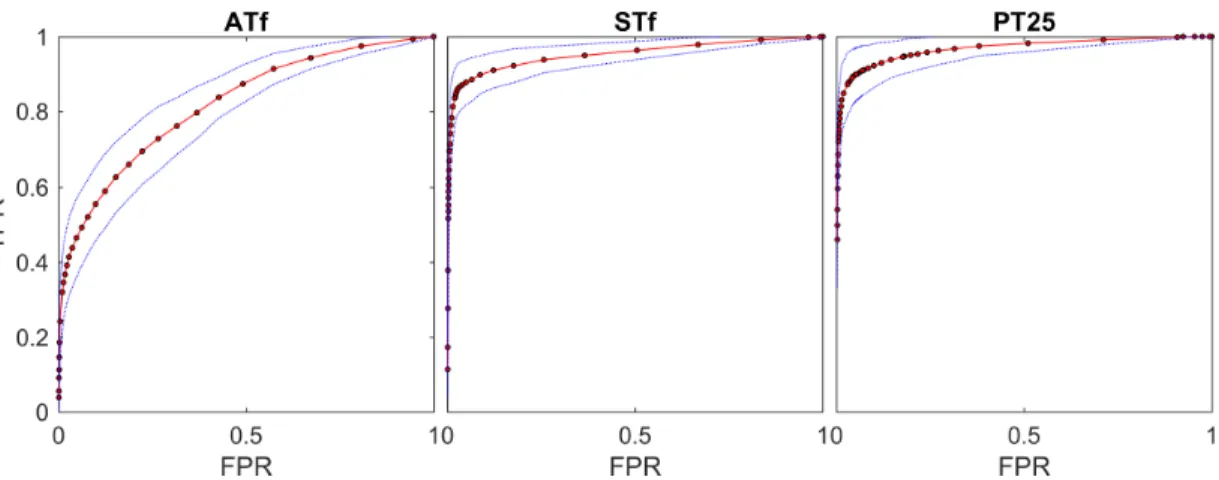
very simple methods. We got the best performance of artifact detection with
thresholding slope, power in high frequency (25-90 Hz or 45-90 Hz) and the
residual errors of an autoregressive model fitted to the EEG. It is not surprising
that the power in high frequency range was a good predictor of an artifact as
muscle artifacts are characterized by the power in high frequency range. Most
methods showed good sensitivity. However, since we had chosen fixed false
4
positive rate (FPR) of 10%, we excluded on average 16.3% of the epochs
whereas experts excluded on average only 7% of the epochs. Our approach
seemed reasonable as it leaves enough data for subsequent analyses.
The main chapter (third chapter) describes the developed automatic
sleep scoring algorithms. Scoring rules are complex and to some degree
subjective. Despite the fact that human brain has superb image recognition
abilities, sleep scoring is a difficult task. Thus, it is not possible to just program
an algorithm which implements the scoring rules for sleep. Such a problem can
be addressed however, with modern machine learning methods. Such
algorithms learn from the examples which have already been analyzed by an
expert. With these techniques we don’t even need to know how to score sleep
stages ourselves, we just need examples of experts. We developed several
algorithms ranging from basic machine learning tools to deep artificial neural
networks. First, we engineered 20 features derived from EEG, EOG and EMG
data. This process reduces the dimensionality of our data and makes
classification of the data easier. We employed a random forest (RF) classifier in
conjunction with a Hidden Markov Model (HMM) or a moving median filter
(MF) to smooth the data. Alternatively, we applied artificial neuronal networks
(ANN), Long-Short Term Memory (LSTM) networks, designed to handle time
series to classify the data. We used our engineered features as input for these
networks. Finally, we employed deep convolutional neural networks (CNNs) in
combination with LSTM networks. Such algorithms (CNN-LSTM networks) work
with raw data and do not require engineered features. We used the F1 score, a
performance measure of multi-class data which takes both specificity and
sensitivity into account, to evaluate the quality of the automatic scoring. We
achieved a sleep stage classification quality close to the human expert in
recordings of healthy subjects, with F1 scores above 0.8 for all stages except
5
for stage 1. Stage 1 is difficult to score for a human scorer as well. F1 scores of
stage 1 were slightly above 0.4 for most our methods, like the interscorer
performance. Our methods trained on healthy participants performed slightly
worse on the patient data than on the data of healthy subjects when they
were trained only on the data of healthy subjects. However, the performance
of the ANNs was better than RF in this case. Performance on the patient data
improved when patient data were included into the training. We
demonstrated that the methods which incorporate the temporal structure
generally perform better. Further, the methods relying on the raw data
performed slightly better than the feature-based methods. We think that we
could not use the whole potential of ANNs due to the scarcity of the training
data.
Using these algorithms, we may score sleep fully automatically and
analyze big amounts of data very quickly. Our CNN-LSTM network produced
good results using just a single EEG channel. This was an unexpected result as
we assumed that reliable detection of REM sleep would require EOG and EMG
data. Such networks would allow on-line scoring of data recorded with
portable devices.
The fourth chapter is dedicated to the automatic detection of
microsleep episodes (MSE). MSE are very short sleep fragments lasting 3 to
15 s. They often occur in sleep deprived people, in individuals who had
insufficient sleep or under boring or monotonous conditions, and in patients
with excessive daytime sleepiness. We engineered features and applied basic
machine learning methods (support vector machine, random forest) to detect
MSE. In a preliminary step we demonstrated that the methods work and
reached very good specificity (0.99) and good sensitivity (0.74). Future
improvement of MSE detection algorithms should include the temporal
6
structure of the data, for example using LSTM neural networks. In summary,
our preliminary analysis provides proof of concept that automatic detection of
MSE based on sleep EEG data is feasible.
All together, we could demonstrate that machine learning approaches
perform well in detecting sleep stages and MSE.
The final chapter provides an outlook on further improvements and
future steps to be taken.
7
Zusammenfassung
Schlaf ist etwas ganz Natürliches. Ein Mensch verbringt etwa ein Drittel
seines Lebens schlafend. Doch trotz all der beeindruckenden Fortschritte in
diesem Bereich ist die Funktion des Schlafs noch immer nicht bekannt. Wir
wissen jedoch, dass Schlafstörungen sich nachteilig auf die Gesundheit und die
Lebensqualität auswirken. Eine der häufigsten Schlafstörungen ist die
Insomnie. Exzessive Tagesschläfrigkeit und ungenügender Schlaf verringern die
kognitive Leistungsfähigkeit und können zu Unfällen führen. Diese Tatsachen
zeigen, dass das Verständnis von Schlaf und seiner Regulation eine wichtige
Rolle spielt.
Im ersten Kapitel dieser Arbeit habe ich die neuesten Hypothesen über
die Funktionen des Schlafs zusammengefasst. Anschließend bin ich auf die
Polysomnographie
(PSG),
den
sogenannten
Goldstandard
in
der
Schlafdiagnostik,
die
Schlafstadien
und
insbesondere
auf
das
Elektroencephalogramm (EEG) eingegangen. Ferner wird ein Überblick über
die «Machine-Learning»-Methoden gegeben, da diese für die Klassifizierung
der Schlafphasen und die Erkennung von Mikroschlaf-Episoden verwendet
werden.
Im zweiten Kapitel haben wir 14 einfache Methoden zur Erkennung von
Artefakten an zwei Datensätzen eingehend getestet. Der erste Datensatz
umfasste Schlaf-EEG-Ableitungen von gesunden jungen Probanden, der zweite
Daten von Patienten, die unter Hypersomnie und Narkolepsie leiden. Wir
haben festgestellt, dass sich mittels dieser sehr einfachen Methoden qualitativ
gute mittlere leistungsdichte Spektren des EEGs ergeben. Die besten
Ergebnisse bei der Artefakterkennung haben wir durch die Begrenzung der
Steilheit der EEG-Auslenkung, der hochfrequenten Leistung im EEG (25-90 Hz
oder 45-90 Hz) oder Abweichungen (residuals) von autoregressiven Modellen,
8
mit denen die EEG-Signale modelliert wurden, erzielt. Es ist nicht
verwunderlich, dass sich die hochfrequenten Komponenten als ein guter
Prädikator für das Vorhandensein eines Artefakts erwiesen, da aus der
Literatur bekannt ist, dass sich Muskelartefakte durch eben diese
Komponenten auszeichnen.Die meisten Methoden wiesen eine gute
Sensitivität auf. Allerdings wurden aufgrund der Tatsache, dass wir eine
Falsch-Positiv-Rate von 10 % festgelegt haben, durchschnittlich 16,3 % der Epochen
ausschlossen, während Experten lediglich durchschnittlich 7 % ausschlossen.
Dies schien uns angemessen, da noch genügend Daten war für die
nachfolgenden Analysen zur Verfügung standen.
Im Hauptkapitel (drittes Kapitel) werden die entwickelten Algorithmen
zur automatischen Schlafstadienbestimmung dargelegt. Die Regeln zur
Bestimmung der Schlafstadien sind komplex und zu einem gewissen Grad
subjektiv. Trotz der Tatsache, dass das menschliche Gehirn über
ausgezeichnete Fähigkeiten zur Bilderkennung verfügt, erweist sich die
Stadienbestimmung selbst für einen Menschen als ein schwieriges
Unterfangen. Demzufolge ist eine manuelle Programmierung eines
Algorithmus, der Regeln zur Bestimmung der Schlafstadien umsetzt, nicht
möglich. Dieses Problem kann mittels moderner
«Machine-Learning»-Methoden angegangen werden. «Machine-Learning»-Algorithmen lernen aus
Beispielen, die bereits von einem Experten klassifiziert wurden. Dank dieser
Methoden sind keine Kenntnisse in Bezug auf die Auswertung der
Schlafphasen erforderlich. Wir benötigen lediglich Beispiele von Experten. Wir
haben mehrere Algorithmen entwickelt, von grundlegenden
«Machine-Learning»-Methoden bis hin zu künstlichen neuronalen Netzen («deep
learning»). Zunächst haben wir 20 sogenannte «Features» auf Grund von EEG-,
EOG- und EMG-Daten bestimmt, wodurch die Dimensionalität der Daten
9
verringert und ihre Klassifizierung vereinfacht wurde. Anschließend haben wir
den sogenannten «Random-Forest»-Algorithmus (RF) verwendet und ein
«Hidden-Markov-Model» (HMM) sowie einen Medianfilter (MF) zur Glättung
der Daten angewandt. Danach haben wir ein künstliches neuronales Netz zur
Verarbeitung von Zeitreihen, das sogenannte
«Long-Short-Term-Memory»-Netz (LSTM), verwendet. Als Input für diese «Long-Short-Term-Memory»-Netze dienten unsere entwickelten
Features. Zum Schluss haben wir «Convolutional Neural Networks» (CNNs)
zusammen mit einem LSTM Netzwerk angewandt. Ein solcher Algorithmus (wir
bezeichnen diesen Algorithmus als CNN-LSTM) arbeitet mit Rohdaten und
bedarf keiner entwickelten Features. Wir haben das F1-Mass, eine Messgrösse
die Spezifität sowie Sensitivität bei mehrfach Klassen einbezieht, verwendet
um die Qualität der automatischen Stadienerfassung zu beurteilen. Die
Ableitungen der gesunden Probanden wiesen mit allen genannten Methoden
eine hohe Schlafphasenklassifikationsgüte auf, die der von Experten entsprach.
Bei den gesunden Probanden erzielten wir für alle Schlafstadien, mit
Ausnahme von Stadium 1, ein F1-Mass von über 0,8. Auch für einen Menschen
erweist sich die Erfassung von Stadium 1 als ein schwieriges Unterfangen. Bei
den meisten unserer Methoden belief sich das F1-Mass für Stadium 1 auf etwa
0,4 wie das auch für die Übereinstimmung zwischen Experten zutrifft. Wir
haben gesehen, dass, wenn unsere Methoden ausschliesslich mit Daten
gesunder Probanden trainiert wurden, die Qualität der Klassifizierung mit
diesen Methoden bei Patientendaten etwas geringer war als bei den Daten
gesunder Probanden. Jedoch erwiesen sich in diesem Fall die künstlichen
neuronalen Netze als leistungsfähiger als der RF-Algorithmus. Mit der
Einbeziehung der Patientendaten in das Training verbesserte sich auch die
Qualität der Klassifizierung bei Patientendaten. Wir haben nachgewiesen, dass
die Methoden, die zeitlichen Strukturen der Daten einbeziehen, im
10
Allgemeinen eine bessere Qualität aufwiesen. Darüber hinaus erwiesen sich
die auf Rohdaten gestützten Methoden als leistungsfähiger als die
Feature-basierten Methoden. Unsers Erachtens nach war es uns aufgrund der geringen
Menge an Trainingsdaten nicht möglich, das Potenzial der künstlichen
neuronalen Netze voll auszuschöpfen.
Diese
Algorithmen
ermöglichen
uns
eine
voll
automatische
Schlafstadienerfassung sowie eine äusserst schnelle Analyse grosser
Datenmengen vorzunehmen. Entgegen unserer Annahme, dass für eine
zuverlässige Erfassung des REM-Schlafs sowohl EOG- als auch EMG-Kanäle
erforderlich sind, erzielte unser CNN-LSTM-Netz unter Verwendung eines
einzigen EEG-Kanals sehr gute Ergebnisse. Solche Netzwerke erlauben eine
«on-line» Klassifizierung von Schlafdaten die mittels portablen Geräten erfasst
werden.
Im vierten Kapitel wird die automatische Erfassung der
Mikroschlaf-Episoden (MSE) behandelt. Bei MSE handelt es sich um kurze Schlaffragmente
von 3 bis 15 Sekunden, die nach Schlafentzug oder ungenügendem Schlaf,
während monotonen Tätigkeiten oder bei Patienten mit exzessiver
Tagesschläfrigkeit auftreten können. Für die Erkennung von MSE haben wir
Features entwickelt und grundlegende «Machine-Learning»-Methoden
(«support vactor machines», «random forest») angewandt. In einem ersten
Schritt haben wir gezeigt, dass die Methoden funktionieren und eine sehr gute
Spezifität (0,99) und eine gute Sensitivität (0,74) aufweisen. Die Algorithmen
zur MSE-Erfassung können zukünftig durch Einbezug der zeitlichen Struktur der
Daten, zum Beispiel durch die Verwendung eines LSTM Netzes, verbessert
werden. Wir haben einen «proof of concept» geliefert, dass die automatische
Erkennung von MSE mittels EEG möglich ist.
11
Insgesamt konnten wir nachweisen, dass sich
«Machine-Learning»-Ansätze bei der Erkennung von Schlafphasen und MSE als äußerst
leistungsfähig erweisen.
Im letzten Kapitel wird ein Ausblick auf weitere
Verbesserungs-möglichkeiten und zukünftige Entwicklungsschritte gegeben.
12
Acronyms
A1
Electrode on the left mastoid (behind the ear)
A2
Electrode on the right mastoid (behind the ear)
AASM
American Association for Sleep Medicine
ANN
Artificial Neural Network
AR
Autoregression
AUC
Area under the curve
BSS
Blind Source Separation
C3
central EEG electrode on the left hemisphere
C3A2
EEG channel C3-A2
CNN
Convolutional Neural Network
DAE
Denoising Autoencoder
DNN
Deep Neural Network
ECG
Electrocardiogram
EEG
Electroencephalogram
EMG
Electromyogram
EOG
Electrooculogram
F3
frontal EEG electrode on the left hemisphere
FFT
Fast Fourier Transformation
FNR
False Negative Rate
FP
False Positive
FPR
False Positive Rate
FPR
False Positive Rate
GD
Gradient Descent
GPU
Graphic Processing Unit
HMM
Hidden Markov Model
Hz
Hertz
ICA
Independent Component Analysis
KM
k-Means
L1
Manhattan norm
L2
Euclidian norm
LASSO
Least Absolute Shrinkage and Selection Operator
LOC
Left Ocular Channel
LSTM
Long-Short Term Memory
MC
Mean Crossing
MF
Median Filter
ML
Machine Learning
MSE
Mean Square Error
13
MT
Movement Time
MWT
Maintenance of Wakefulness Test
N1
Sleep stage 1 (light sleep)
N2
Sleep stage 2
N3
Sleep stage 3 (deep sleep; SWS)
NLP
Natural Language Processing
NREM
Non Rapid Eye Movement
PCA
Principal Component Analysis
PSG
Polysomnography
REM
Rapid Eye Movement
RF
Random Forest
RNN
Recurrent Neural Network
ROC
Right Ocular Channel
ReLU
Rectified Linear Unit
SAE
Stochastic Autoencoder
SEF
Spectral Edge Frequency
SEM
Slow Eye Movement
SGD
Stochastic Gradient Descent
SOREM
Sleep Onset Rapid Eye Movement
SPC
Specificity
SSRI
Selective Serotonin Reuptake Inhibitors
SVM
Support Vector Machine
SWA
Slow Wave Activity
SWS
Slow Wave Sleep (stages 3 and 4)
SpO2
Blood oxygen saturation
TN
True Negative
TP
True Positive
TPR
True Positive Rate
VAE
Variational Autoencoder
ZC
Zero Crossing
fMRI
functional Magnetic Resonance Imaging
fs
sampling frequency
t-SNE
t-distributed Stochastic Neighbor Embedding
14
Acknowledgements
I relied on the help of many people during my PhD. First of all I
acknowledge Prof. Dr. Peter Achermann. He gave me a chance to accomplish
the PhD. Peter created comfortable and nourishing environment. Peter, I
learned from you many things. Not only scientifically, but also on the personal
level. Experience during this PhD tremendously changed many aspects of my
thinking. I had a unique opportunity to develop my ideas in comfortable
environment. I am very grateful to Prof. Dr. Alexander Borbély and
Prof. Dr. Irene Tobler for teaching me a lot and helping out. This work would
not be possible without help and support of my thesis committee members
Prof. Dr. Peter Achermann, Prof. Dr. Kevan Martin and Prof. Dr. Thomas König.
I am extremely grateful to my friends Dr. Dmitry Laptev, Valentina
Lapteva, Dr. Valery Vishnevsky, Alexander Kolesnikov, Lera Kolesnikova, Arseny
Klimovsky, Nikolay Savinov, Alexey Gronsky and Elena Gronskaya and all other
friends for being around and supporting me.
This work would not have been possible without contributions from my
collaborators Dr. Dmitry Laptev, Dr. Stefan Bauer, Dr. Ximena Omlin,
Dr. Aleksandra Wierzbicka, Dr. Adam Wichniak, Prof. Dr. Wojciech Jernajczyk,
Prof. Dr. Robert Riener, Dr. Jelena Skorucak and Prof. Dr. Joachim Buhmann.
I am grateful to Jakub Michankow for the permission to use the photo
he made as a cover picture (it was modified).
Dmitry Laptev, Valery Vishnevsky and Lilit Poghosyan helped me
proofreading this thesis. Lilit helped me a lot with the English language in
general. I am very thankful to Anna Neumann for teaching me German.
I am very thankful to all my office and group mates and all the members
of the institute for help and support! I am grateful to Dr. Thomas Rusterholz,
Ueli Wyss and Dr. Roland Dürr for technical support.
I am expressing the greatest gratitude to my parents for raising and
supporting me!
15
Contents
Summary ... 3
Zusammenfassung ... 7
Acronyms ... 12
Acknowledgements ... 14
1 Introduction ... 19
1.1 What is sleep ... 19
1.2 Sleep theories ... 20
1.2.1 Energy conservation ... 20
1.2.2 Cellular maintenance... 20
1.2.3 The memory and synaptic homeostasis hypothesis... 21
1.2.4 Cleaning of “brain waste” ... 21
1.3 Sleep disorders ... 22
1.4 Sleep evaluation ... 23
1.4.1 Electroencephalogram (EEG) ... 23
1.4.2 Electrooculogram (EOG) ... 25
1.4.3 Electromyogram (EMG) ... 26
1.4.4 Breathing effort ... 26
1.4.5 Snoring ... 27
1.4.6 Airflow ... 27
1.4.7 Blood oxygen saturation (SpO2) ... 27
1.4.8 Electrocardiogram ... 27
1.5 Sleep stage scoring ... 28
1.6 Quantitative EEG analysis: spectral analysis ... 30
1.6.1 Slow wave activity (SWA) ... 30
1.6.2 Sleep “fingerprint” ... 30
1.6.3 Benzodiazepine ... 32
1.7 Artifacts ... 32
1.8 Machine Learning ... 34
1.8.1 K-means clustering ... 34
1.8.2 Logistic regression ... 35
1.8.3 Cost function ... 36
1.8.4 The problem of overfitting ... 36
1.8.5 Regularization ... 38
1.8.6 Random Forest ... 38
1.8.7 Boosting ... 40
1.8.8 Artificial neural networks ... 40
16
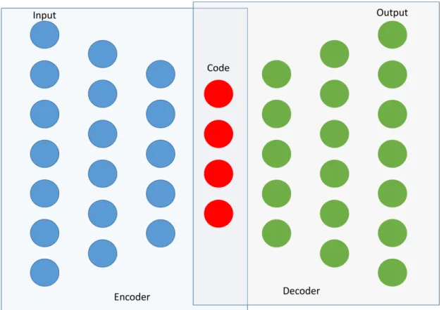
1.8.10 Unsupervised learning ... 47
1.8.11 Performance evaluation ... 50
1.8.12 Validation ... 52
1.9 Automatic sleep scoring ... 53
2. Automatic artifact detection in single channel sleep EEG
recordings ... 56
2.1 Abstract ... 57
2.2 Introduction... 58
2.3 Materials and methods ... 60
2.3.1 Data sets ... 60
2.3.2 Algorithms ... 63
2.3.3 Evaluation of the performance of the algorithms ... 63
2.4 Results ... 65
2.4.1 Derivation of parameters (thresholds) of the algorithms ... 65
2.4.2 Testing of performance on independent data sets ... 68
2.4.3 Effect of artifact exclusion on NREM sleep power density spectra ... 68
2.5 Discussion ... 71
2.6 Conclusion ... 76
2.7 Acknowledgements ... 76
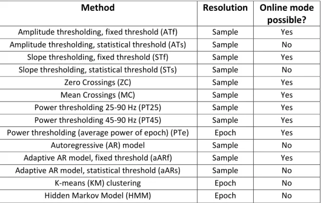
2.8 Supporting Information: Algorithms ... 77
2.8.1 Amplitude thresholding (ATf, ATs) ... 77
2.8.2 Slope thresholding (STf, STs) ... 77
2.8.3 Zero crossings (ZC) ... 77
2.8.4 Mean crossings (MC) ... 78
2.8.5 Power thresholding (PT25, PT45, PTe) ... 78
2.8.6 Autoregressive Model (Inverse filtering; AR) ... 79
2.8.7 Adaptive autoregressive modeling (aARf, aARs) ... 79
2.8.8 K-means (KM) clustering. ... 80
2.8.9 Hidden Markov Model (HMM). ... 80
3 Automatic human sleep stage scoring using Deep Neural
Networks ... 82
3.1 Abstract ... 83
3.2 Introduction... 83
3.2.1 Problem statement ... 83
3.2.2 Related work ... 85
3.2.3 Our contribution ... 88
3.3 Methods ... 89
3.3.1 Polysomnographic (PSG) data ... 89
17
3.3.3 Deep learning with raw data………..94
3.3.4Learning time dependencies………..95
3.4 Study setup ... 98
3.4.1 Network architectures ... 98
3.4.2 LSTM networks ... 98
3.4.3 CNN-LSTM networks ... 97
3.4.4 Optimization... 101
3.4.5 Training, validation, and testing ... 101
3.4.6 Performance evaluation ... 102
3.5 Results ... 102
3.5.1 Convergence of the ANNs ... 102
3.5.2 Classification performance ... 103
3.6 Discussion ... 107
3.6.1 Comparison with human experts and automatic scoring of other
groups ... 107
3.6.2 Automatic scoring using different channels... 109
3.6.3 Is the F1 score a good measure of scoring quality? ... 110
3.6.4 Which method is the best? ... 110
3.6.5 Importance of the training data ... 111
3.6.6 Effect of the length of the sequence ... 112
3.6.7 Room for further improvement ... 112
3.7 Conclusions ... 114
3.8 Acknowledgements ... 115
3.9 Supplementary material ... 115
3.9.1 Definition of features ... 115
3.9.2 Taking the temporal structure into account by a Hidden Markov
Model (HMM) ... 126
3.9.3 Optimization... 127
3.9.4 Batches ... 129
3.9.5 Training and validation ... 130
3.9.6 Naming conventions of algorithms ... 131
3.9.7 Training and validation ... 133
3.9.8 Performance evaluation ... 137
4 Microsleep episode detection ... 148
4.1 Introduction ... 149
4.2 Data and methods ... 149
4.3 Results ... 151
4.4 Conclusion and discussion ... 152
18
5.1 Automatic artifact detection ... 154
5.2 Sleep stage classification ... 157
Bibliography ... 166
Curriculum Vitae ... 185
Published papers and abstracts ... 185
Papers ... 185
Abstracts ... 186
Awards ... 187
19
1 Introduction
1.1 What is sleep
We all sleep, and we have a notion of what sleep is. Sleep may be
defined on a behavioral level or based on electrophysiological (see further
below).
A behavioral definition of sleep was developed by Piéron (Piéron, 1913)
and extended by Flanigan et al. (Flanigan Jr et al., 1974). According to
behavioral definition, sleep is the state when animal is (1) immobilized, (2)
chooses specific place to sleep, for example a nest, (3) has a characteristic
body posture, (4) an animal can be quickly woken up, (5) the animal’s arousal
threshold is higher than in wakefulness, (6) sleep is homeostatically regulated.
The requirement of homeostatic regulation was introduced by Irene Tobler
(Tobler, 1984).
It has been shown that most studied species show clear signs of sleep,
including drosophila (Hendricks et al., 2000), zebrafish (Zhdanova et al., 2001)
and even C. Elegans (Raizen et al., 2008). However, there are certain species
whose sleep is more questionable, for example, the bullfrog (Hobson, 1967).
It is well known that sleep deprivation in human leads to cognitive
impairments (Kjellberg, 1977, Alhola and Polo-Kantola, 2007, Kerkhof and Van
Dongen, 2010, McCoy and Strecker, 2011). It also affects the mood (Banks and
Dinges, 2007). The death of animals after prolonged total sleep deprivation
was observed in several species: rats (Everson et al., 1989), drosophila (Shaw
et al., 2002) and cockroaches (Stephenson et al., 2007).
Interestingly, sleep deprivation can have a positive effect in depressed
patients: it alleviates depression (Giedke and Schwärzler, 2002). However, the
effect disappears after recovery sleep.
20
It seems that sleep is universal and essential. Despite the fact that the function
of sleep is unknown, there are many theories addressing this question
(Rechtschaffen, 1998, Mignot, 2008, Cirelli and Tononi, 2008).
1.2 Sleep theories
1.2.1 Energy conservation
One of the first hypotheses on the function of sleep was an idea that
sleep might have been evolved due to a reduced energy consumption during
this state (Walker and Berger, 1980). However, there is already a state of
torpor which serves as a means of energy conservation and animals experience
a sleep rebound after they come out of torpor (Heller and Ruby, 2004).
Moreover, energy consumption is reduced only in NREM sleep, but not in REM
sleep (Zhang et al., 2007).
1.2.2 Cellular maintenance
Another widely known hypothesis is a recovery hypothesis. It suggests
that sleep is needed to recover cellular structures (Mackiewicz et al., 2007).
Some studies, though, showed that sleep does not affect protein synthesis
(Clugston and Garlick, 1982).
Vyazovskiy and Harris (Vyazovskiy and Harris, 2013) proposed a
hypothesis that neurons have limited capacity to perform information
processing and should undergo cellular maintenance to repair the “wear and
tear” damage. Unless it happens, sleep might intrude into wakefulness to
prevent permanent damage to neurons at cost of reduced performance during
wakefulness. The authors suggested that maintenance can only be performed
when neuron is disconnected from the network activity.
21
1.2.3 The memory and synaptic homeostasis hypothesis
It has been suggested that sleep is crucial for the information
processing.
Tononi and Cirelli came up with the synaptic homeostasis theory (Tononi
and Cirelli, 2006). New synapses are formed during wakefulness due to
learning of new things. At some point, the ability of the brain to form new
synapses saturates. Therefore, the net synaptic strength needs to be adjusted
and decreases during sleep, particularly NREM sleep. According to the synaptic
homeostasis theory, this is the crucial function of sleep.
A number of other studies have shown that sleep facilitates learning and
memory consolidation (Karni et al., 1994, Stickgold, 2006, Born et al., 2006,
Yoo et al., 2007).
It has also been observed that replay of the activations which had
happened during wakefulness may occur during sleep (Pavlides and Winson,
1989, Ji and Wilson, 2007, Stickgold et al., 2001, Diekelmann and Born, 2010).
This phenomena is called hippocampal replay.
1.2.4 Cleaning of “brain waste”
Recent studies conducted by Dr. Maiken Nedergaard and her colleagues
showed that cerebral fluid flow dramatically increases during sleep (Xie et al.,
2013, Iliff et al., 2012). The space between neurons enlarges and more fluid
flows through these clefts. The proposed theory says that it helps to flush out
toxins, particularly beta-amyloid. Brain does not have a lymphatic system and
such a mechanism can be a substitution of the lymphatic system. So far
increase in the cerebral fluid flow has been shown in animals, but not yet in
humans.
22
1.3 Sleep disorders
Sleep is of a big interest for medicine since the prevalence of sleep
disorders is tremendous. According to some studies (Bixler et al., 1979,
Hersberger et al., 2006, Ohayon, 2002), up to 50% of population suffer from
some kind of sleep disorders, mainly, insomnia.
It is clear that sleep affects health: people with disturbed sleep have
increased risk of cancer and it damages immune system (Irwin, 2015).
Moreover, reduced sleep duration leads to metabolic diseases such as type
two diabetes (Copinschi et al., 2014). These patterns have been extensively
studied in shift workers: they have higher risks of cancer, diabetes, depression
and cardiovascular problems (Faraut et al., 2013, Marquié et al., 2014, Ramin
et al., 2015). That is the reason why studies on how changes in sleep influence
human health are of a great importance. The importance of such studies is still
growing because sleep duration has been decreasing over the last several
decades (Tinguely et al., 2014). As a further matter, sleepiness, sleep loss and
excessive daytime sleepiness have been one of the causes of major industrial
accidents (for example Chernobyl) and transportation (Rajaratnam and Arendt,
2001).
Another common sleep disturbance is obstructive sleep apnea (Force
and Medicine, 2009). It affects people's well-being, causes excessive daytime
sleepiness, which leads to accidents on transportation, and increases risks of
developing chronic illnesses.
A lot of other sleep-related conditions require evaluation in a sleep
laboratory. Hypersomnia and narcolepsy are among such disorders (Roth and
Broughton, 1980). Both conditions are manifested in the excessive daytime
sleepiness. Narcolepsy, for instance, can be manifested either in sleepiness
only or in sleepiness combined with sleep attacks and cataplexy. During a
23
cataplectic attack, a person loses muscle tone and collapses; it mostly happens
after experiencing strong emotions
All these conditions require evaluation for diagnosis, treatment and in
some countries fitness to drive must be evaluated and is required for affected
people in order to possess a driving license, particularly for professional
drivers.
1.4 Sleep evaluation
Sleep evaluation is needed both in research and medicine. Research
questions such as sleep regulation, sleep and health etc. require objective
measures. The gold standard of sleep studies is polysomnography, which is a
recording of several biosignals (including at least the first three signals) listed
below.
1.4.1 Electroencephalogram (EEG)
The EEG is the most important state indicator for us. Electrodes on the
scalp measure electrical field potential changes, which result from
postsynaptic potential changes of pyramidal neurons in the cortex (Buzsáki et
al., 2012).
The EEG measures the difference in the potential between two
electrodes. One is placed in the area of the interest – on the scalp, the other
one is the reference electrode. Common references in sleep research and
medicine are the contralateral mastoids (behind the ear). The left mastoid
electrode is named A1, the right one A2.
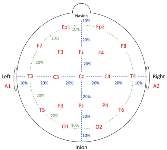
Other EEG electrodes are usually named with a letter and a number.
Letter stands for the location: O-occipital, P-parietal, C-central, F-frontal,
T-temporal. Number also reflects location according to the electrode placement
24
system “10-20 system” (Jasper, 1958) (Figure 1.1). Odd numbers stand for the
left hemisphere, even ones for the right hemisphere and the index z indicates
the midline.
In this way derivations are named after the two electrodes concerned,
for example C3-A2 is the channel which is commonly used for scoring
(Rechtschaffen and Kales, 1968). It means that the potential difference of the
electric field is measured between C3 and A2.
Derivations can be referenced in other ways, for example F3-C3 or an
electrode can be referenced to the average reference (mean of all electrodes
in case of high-density EEG recordings), however we did not work with such
references.
Figure 1.1. Electrode placement according to the 10-20 system. Modified from
”Bits of Sleep” (Borbély et al., 1998)
25
Neuronal activity creates oscillations of different frequencies in the EEG
signal. One of the most widely known oscillations is alpha oscillation. It was
discovered by Hans Berger (Berger, 1929). It is an oscillation with a frequency
around 10 Hz. Alpha oscillations appear in relaxed wakefulness with closed
eyes. When the subjects open their eyes, alpha oscillations generally disappear
(alpha blocking).
Delta (slow) waves are oscillations in the frequency range of 0.5 – 4 Hz.
They were discovered by Walter Grey (Walter, 1936). Slow waves are the
marker of deep sleep (Rechtschaffen and Kales, 1968).
EEG power in the range 0.5-4.5 Hz is called slow-wave activity (SWA).
SWA is homeostatically regulated and one can observe a rebound after sleep
deprivation (Borbély et al., 1981, Borbély and Achermann, 1999).
Another important oscillation is a sleep spindle. This is a waxing and
waning oscillation in the frequency range 12-14 Hz with a duration of 0.5 to 2 s
(Rechtschaffen and Kales, 1968). Sleep spindles are a main property of the
sleep stage 2 (see below).
1.4.2 Electrooculogram (EOG)
Electrodes located on the skin near the eyes record changes in the
potential of electric field due to the eye movement. This change in the
potential is caused by the fact that eye is a dipole (Marg, 1951). Eye
movements are essential to score sleep because every sleep stage has distinct
patterns of eye movements.
Usually two EOG channels are used. One electrode is located above the
outer canthus (corner) of the left eye. This channel is called Left Ocular
Channel (LOC). It is usually referenced to one of the mastoids (A1 or A2). The
26
other electrode is located below the outer canthus of the right eye. This
channel is called Right Ocular Channel (ROC).
Rapid Eye Movements (REMs) are one of the most prominent properties
of REM sleep and they are manifested in anticorrelated deflections in LOC and
ROC.
Eye blinks occur only during wakefulness and are helpful to distinguish
this stage. Eye blinks also cause anticorrelated deflections in the LOC and ROC,
but the shape of the signal is different. We observed that there are two
different types of eye blinks: (1) when deflections in the LOC and ROC have the
same amplitude and (2) when deflection in the LOC has a larger amplitude
than the one in the ROC. We did not find reports on this phenomena in the
literature. I think it happens because electrodes during eye blink record rather
the activity of the muscles than the polarization of the eyeball. And there
might be two distinct patterns of muscle activation for the eye blinks (see
chapter 3.9.1).
1.4.3 Electromyogram (EMG)
Electrode placed on the muscle measures its activity, i.e. muscle tone. In
sleep research it is common to record muscle tone from the electrodes located
under the chin (submental EMG). Muscle tone is lower during sleep than
during wakefulness. REM sleep is characterized by extremely low muscle tone,
also known as REM sleep atonia (Jouvet et al., 1959, Rechtschaffen and Kales,
1968).
1.4.4 Breathing effort
Breathing effort is routinely measured by two belts, one located around
the chest, the other is placed lower, measuring movement of the abdomen.
27
These belts detect changes in their length. Breathing in leads to a lengthening,
breathing out to a shortening. In the case of obstructive sleep apnea, doctors
see an increased breathing effort along with a drop in blood oxygen saturation
and a cessation of airflow.
1.4.5 Snoring
Snoring can be recorded using a microphone. This signal is important in
clinical setting. We did not use it in our studies.
1.4.6 Airflow
The airflow through the nose and mouth may be recorded using
temperature sensor located below the nose. The exhaled air is warmer than
the inhaled one.
1.4.7 Blood oxygen saturation (SpO2)
An important measure for screening patients for sleep apnea is blood
oxygen saturation. It is usually measured at the fingertip. SpO2 drops when
episodes of apnea occur.
1.4.8 Electrocardiogram
Electrocardiogram registers electric activity of the heart. It can be useful
for sleep analysis and particularly for detection of sleep apnea events
(Sivaranjni and Rammohan, 2016) and this signal may be used to correct
cardiac artifacts in EEG channels.
28
1.5 Sleep stage scoring
A recording is minimally composed of the EEG, EOG and EMG signals.
Further, these signals are evaluated by a professional. The recording is being
split into 20- or 30-s long intervals, the scoring epochs. They are visually scored
as wakefulness, sleep stages 1, 2, 3 and 4, and so-called paradoxical or
rapid-eye movement (REM) sleep.
REM sleep was first found in cats by Rudolf Klaue in 1937 (Klaue, 1937),
distinct electrical activity during dreaming was also observed by Loomis
(Loomis et al., 1935, Loomis et al., 1937, Loomis et al., 1938). The first paper
with the study of this state was published by Aserinsky and Kleitman (Aserinsky
and Kleitman, 1953). They coined the term Rapid Eye Movement (REM) sleep.
At about the same time French scientist Michel Jouvet and his
colleagues observed muscle atonia in cats accompanied by sporadic twitches.
They called it “paradoxical sleep”. The paper (Jouvet et al., 1959) was
published only some years after their discovery.
Sleep is being scored according to the scoring manuals. The first manual
was published in 1968 by Rechtschaffen and Kales (Rechtschaffen and Kales,
1968). According to this manual, sleep was classified into wake, non-rapid eye
movement (NREM) sleep stages 1, 2, 3, and 4, REM sleep and movement time
(MT), i.e. when a subject moved and a signal was contaminated with
movement artifacts. Stages 3 and 4 are considered as slow wave sleep (SWS,
deep sleep).
In the novel scoring rules published by American Association of Sleep
Medicine (Iber et al., 2007), basically SWS was named N3, no longer subdivided
leading to the NREM sleep stages N1 to N3, and MT was abolished.
In my opinion, stage MT is important because otherwise it is not clear
how to score such epochs contaminated by an artifact, especially when it
29
comes to automatic scoring algorithms. I noticed that these epochs were often
recognized by an algorithm as wakefulness, which definitely makes sense. In
this case, though, we have clear discrepancy between an expert and the
computer. Experts usually score such epochs as the same stage as the
surrounding sleep.
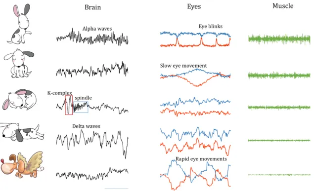
Examples of distinct EEG, EOG and EMG patterns in the different sleep
stages are illustrated in Figure 1.2.
Figure 1.2. This figure shows examples of the EEG, EOG and EMG signals in the
different sleep stages (from top to bottom: Wake, Stage 1, 2, 3, REM). Images
from following sources were used: Natasha_Chetkova/Shutterstock; Alina
Odryna/Shutterstock
In order to score a sleep recording, an expert splits the recording into
consecutive into 20- or 30-s long intervals and assigns the stage based on the
patterns the expert sees in the signals. This process is very time consuming,
and, according to several studies (Danker-Hopfe et al., 2004, Penzel et al.,
2013, Rosenberg and Van Hout, 2013, Younes et al., 2018), human experts are
prone to make mistakes and have a lot of disagreement with each other. For
30
this reason, a number of attempts were undertaken to score sleep
automatically. However, no standard has yet been established.
1.6 Quantitative EEG analysis: spectral analysis
Hypnograms and visual representation of PSG signals provide good
overview of the sleep structure and can be used by medical doctors to
diagnose many sleep disorders. For many applications it is not enough to have
qualitative description of the data. Certain research and clinical questions can
be better addressed using quantitative analyses. One of the most widely used
quantitative measures of sleep are EEG power density spectra. Several
important parameters can be derived from the spectra. Some of them are
listed below and in Figure 1.3.
1.6.1 Slow wave activity (SWA)
First of all one can compute power in the low frequency range (0.75 - 4.5
Hz), called slow wave activity (SWA) which is a reliable marker of sleep
homeostasis (Borbély and Achermann, 1999).
1.6.2 Sleep “fingerprint”
Average power spectra of distinct sleep stages are quite an interesting
characteristic of sleep. It was shown that average spectra were very stable and
may be considered as a sleep “fingerprint” (Lennox et al., 1945, Stassen, 1980,
Buckelmüller et al., 2006, Bersagliere et al., 2018). Sleep EEG power density
spectra were very similar in monozygotic twins (De Gennaro et al., 2008).
31
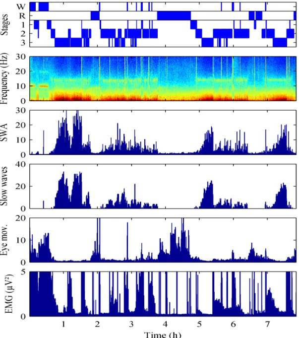
Figure 1.3.
This figure shows the recording of a night of sleep and extracted
quantitative parameters (features). Panel 1: sleep hypnogram; Panel 2:
spectrogram; Panel 3: slow wave activity (SWA); Panel 4: the number of high
amplitude slow waves per epoch; Panel 5: SWA of the ocular channel
(LOC-ROC) divided by SWA of the EEG; Panel 6: Power in the chin EMG. The figure is
from a conference abstract (Achermann et al., 2015)
32
1.6.3 Benzodiazepine
Certain drugs affect average power spectra. Benzodiazepines reduce
slow wave activity and enhance spindle activity (Trachsel et al., 1990, Tobler et
al., 2001). This is also true for Z-drugs (analog substances) (Brunner et al.,
1991). Such changes in the power density spectra are very similar for the
different drugs, also called the spectral signature of benzodiazepines and
analogs. The example of the change of the power spectra, caused by three
drugs, relative to placebo is illustrated in Figure 1.4 Trachsel et al., 1990,
Brunner et al., 1991, Borbély et al., 1998).
1.7 Artifacts
Artifacts are detrimental for both quantitative spectral analysis and for
automatic scoring. It is necessary to identify epochs with artifacts and exclude
them from spectral analysis. It is very useful to perform it automatically.
In this work, we addressed both automatic artifact detection and
automatic sleep scoring. A number of attempts to solve the problems of
artifact detection have been made for some time now (Ktonas et al., 1979,
Barlow, 1983, Barlow, 1984, Barlow, 1986, Bodenstein and Praetorius, 1977,
Gotman et al., 1981, Durka et al., 2003) (D’Rozario et al., 2015, Coppieters’t
Wallant et al., 2016).
Fortunately, nowadays we can tackle these issues with novel methods as
machine learning methods have advanced with an enormous pace. Artificial
neuronal networks were proven to be superior to classical machine learning
methods (decision trees (Safavian and Landgrebe, 1991), Support Vector
Machines (SVMs) (Cortes and Vapnik, 1995), logistic regression etc.) for most
types of data.
33
Figure 1.4. Effect of three sleep medications on the NREM sleep EEG power
spectra. The change is relative to the placebo condition. Blue color covers
frequency range with a statistically significant difference. Figure modified from
(Borbély et al., 1998)
34
1.8 Machine Learning
A newly appeared branch of computer science, called Machine Learning,
allows computers to learn how to label data without either directly
programming the classification rules or even knowing them.
Machine learning can also be used to solve regression and clustering
problems. If we want to assign labels to the data and we have the so-called
training set, i.e. dataset with labeled examples available, it is a classification
problem.
In case we do not have training set with labels we can perform a
clustering. For example, we have data points in some space and we want to
group them. The algorithm groups the data in a way that, for example, the sum
of some metric (for example Euclidian distance) between the point and the
center of a corresponding group is minimal. One of the most widespread
algorithms to solve this problem is K-Means (Steinhaus, 1956). This algorithm
arranges data into K clusters.
If we have examples of labeled data, we should use classification
algorithms. The algorithm will learn statistical properties of the dataset and
“understand” how to label new data points. Such type of learning from the
data labeled by an expert is known as supervised machine learning.
1.8.1 K-means clustering
This is the most widely known clustering algorithm. We can describe
every data point by a vector of the length d (dimension). For instance, we have
patient data and we measured temperature and height, in this case d=2. We
can plot our points in a two-dimensional plane (Fig. 1.5).
The idea is to split the feature space into k segments in a way that every
segment contains a similar number of data points. The algorithm is iterative.
35
Let us choose k centroids randomly. They will be centers of our clouds of
points. Then we will split the space into two parts with a line in a way that the
distance from the line to both centroids is the same. In the case of
multidimensional space it will be a multidimensional surface. We will assign
the labels to the points that all the points on one of the sides belong to the
class of corresponding centroid on the same side. Then we recalculate
coordinates of centroids and repeat the procedure until it converges.
Figure 1.5.This figure shows an example of two-dimensional data of healthy
and ill people
1.8.2 Logistic regression
The simplest approach to do a classification is the logistic regression
(Cox, 1958). It is similar to simple linear regression but the value of the
function belongs to the interval [0, 1]. The logistic function is shown below:
36
!"#$ =
''()*"+,-+./$
(1.1)
A subtype of a logistic function is a sigmoid function which is widely used
in neural networks as an activation function.
1.8.3 Cost function
After we fit a linear regression, we usually use mean square error (MSE
or L2 norm) to understand if the fit is good. Moreover, the fitting procedure is
minimizing the MSE. Such a measure is called a cost function. It tells us how
much mistakes cost. It does not necessarily have to be an MSE, it can be, for
example, a sum of absolute values of errors (L1 norm). Cross-entropy is also a
commonly used loss function for classification purposes (De Boer et al., 2005).
Cross entropy provides a good measure of errors when our targets are discrete
and we predict probabilities. Assume we have an epoch of sleep labeled as
REM sleep. Then target probability is 1. And we predict probability p. If p is
close to 1 then cross entropy loss is close to zero. If p is close to 0 then cross
entropy loss is very big and it increases non-linearly because it is based on the
logarithmic function.
1.8.4 The problem of overfitting
If we want to fit a straight line into a set of points, we use only two
parameters and the result looks like the one on the Fig. 1.6 (top). The data
used for fitting are represented by the blue dots. The red dots show new data
points from the same distribution.The fitted line catches the trend but there is
a certain discrepancy between the data points and the corresponding values of
the linear function. We can add quadratic term, cubic term etc. to our
function. In the end we can have a function which goes exactly through every
37
point (Fig. 1.6 middle). You can see that one red dot is very far from the fitted
line in the middle panel. Despite that, the line goes exactly through every blue
point where the error is 0. But if we add new points on the plot we can see
that the errors for the new data may become large. This case is called
overfitting. Our model was fitted to irrelevant noise in the dataset. This also
means that our model has a high variance. On the contrary, the first model is
too simple, or, in other words, it has bias. The trade-off between the too
simple and too complex models is called bias-variance trade-off. A case of a
good bias-variance trade-off is shown in the Fig. 1.6 (bottom). There we fitted
a quadratic function.
Figure 1.6. Fitting of polynomials of order 1, 20 and 2 to the data (blue circles).
Red circles are new data points drawn from the same distribution
38
1.8.5 Regularization
The problem of overfitting can be addressed by regularization methods.
The simplest method is to assign a penalty to the coefficients. It can be, for
example, the sum of the squares of the polynomial coefficients multiplied by a
regularization parameter λ.
The idea is that polynomial functions with larger coefficients can have
larger variance in order to accommodate every data point. This type of
regularization is called L2 or ridge regularization.
Another way is to use the sum of the absolute values instead of the
squared ones. This is called L1 regularization or LASSO (Tibshirani, 1996).
L1 regularization assigns zeros to small coefficients. That’s the most important
property. It can be used for both feature selection and efficient removal of
irrelevant features from the model.
1.8.6 Random Forest
Decision trees are widely used to solve classification problems (Morgan
and Sonquist, 1963, Hunt et al., 1966, Breiman et al., 1984). A decision tree is a
way to represent a set of rules. On every node of a decision tree a split on
certain feature is being performed. The threshold is stored in the node. In
order to assign a label to a data point, one has to go down the tree and
compare the value of a corresponding feature to a threshold. Outcome of the
comparison determines into which branch of the tree we go next. When the
tree is traversed, we end up in the leaf which defines the corresponding label
of a feature.
A decision tree is a good and simple method, but it is not robust to
outliers. It means that outliers can affect the structure and performance of the
tree. A way to overcome this problem is to use a set of trees: build number of
39
trees, an ensemble (random forest, RF). Each tree is built using a random
subset of the data and a random subset of features (Ho, 1995, Breiman, 2001).
Choosing a random subset of features is called feature bagging. While a tree is
being grown, a feature for every new node is chosen in a way to maximize
information gain.
This allows us to compute importance of features. In order to label new
data point each tree assigns its own label. The eventual label is produced by
“voting” of the trees. Probability of the point belonging to each class can also
be computed. This probability is equal to the number of trees which assigned
the data point to the corresponding class divided by the total amount of trees.
The RFs are superior to machine learning methods which use metric to
compute distance between features because RFs are insensitive to
renormalization, scaling and nonlinear monotonous transformations of
features. In case of Support Vector Machine (SVM) (Cortes and Vapnik, 1995),
features should be normalized. For example, we have temperature of a person
in Celsius and height in millimeters. We want to classify ill and healthy people.
Obviously temperature is an important feature and the height is irrelevant.
Moreover, height is a kind of noise in this case. However, the variation of the
height in millimeters will be much larger than the variation of the temperature
in °C. Thus, distance between the two points will be driven by height, i.e. noise.
For the RF, height will be irrelevant, it will quickly find out that temperature
provides a larger information gain. Irrelevant features and noisy features can
often be found in biological data.
The RF approach is very good for selecting relevant features due to
feature bagging. One has to be aware that in case many correlated features
are present, feature selection will not have a unique solution. Presence of
correlated features is often the case in biology. We observed it in our data too.
40
It does not affect the quality of classification. Still, it would be a big issue if one
wants to find out relevant features or establish causal relationships. As for
correlated features, they can be decorrelated using principal component
analysis (PCA) (Pearson, 1901).
Among other advantages, the RF classification has is the ability of
learning complex rules. It also requires less hyperparameters (only the number
of trees) and performs well in a wide range of this parameter. Oshiro et al.
(Oshiro et al., 2012) studied the performance of RF on several datasets and
found that the performance saturated at number of trees 64 or 128. Of course
for different applications it may vary.
1.8.7 Boosting (Chen and Guestrin, 2016)
Imagine the following situation. You drop matches out of the box on the
table. Then you ask a friend to estimate how many matches are on the table.
The answer is unlikely to be precise. On the other hand, if you ask many
friends independently and average their answers, you will get a good estimate
of amount of matches. The same idea can be applied to classification: if we
have a bunch of weak classifiers, we can average the outcome of classification,
and the result will be better than the result of each of these classifiers. This
method is called boosting and RF classification is an example of such a method.
1.8.8 Artificial neural networks
Modeling a neuron
in silico has
always been a fascinating thing to do
.
A
lot of models had been proposed (Farley and Clark, 1954, Rochester et al.,
1956) which were early on used for data classification (Rosenblatt, 1958).
These models were eventually extended. And this, in its turn, has led to the
41
introduction of multilayer neural networks (Widrow and Hoff, 1960). These
networks are now called artificial neural networks (ANNs).
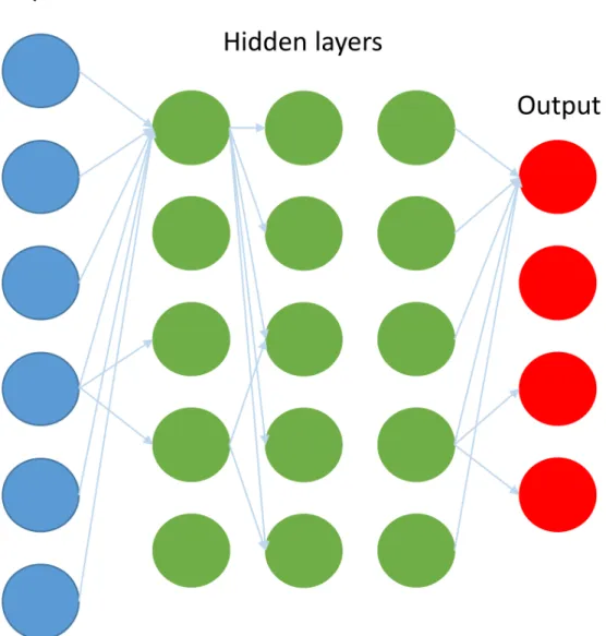
ANNs are comprised of interconnected neurons (an example of an ANN
is illustrated on the Figure 1.7). Each neuron calculates the weighted
summation of the inputs. Weights are the parameters of a neuron. Weights
shall be adjusted during training of the network. It has become possible to
train large networks since the backpropagation (Werbos, 1974) algorithm was
invented. The backpropagation algorithm helps to compute gradients. Weights
are modified using the gradients by gradient descent algorithm or, for
example, the Adam (Adaptive moment estimation) algorithm (Kingma and Ba,
2014).
In order to solve the problem of image recognition, artificial neural
models were proposed. The very first work of Fukushima et al. (Fukushima and
Miyake, 1982) was inspired by studies of Hubel and Wiesel (Hubel and Wiesel,
1959). Fukushima’s algorithm is the first algorithm which resembled a
Convolutional Neural Network (CNN).
The CNN in its modern form was discovered and popularized later by
LeCunn et al. (LeCun et al., 1989) and Waibel et al. (Waibel et al., 1989). As the
name suggests, such ANNs perform a convolution of input data (image) with a
set of filters. These filters are adjusted during training. Convolution can be
described in the following way: a window with some picture is moved across
the input image. The picture on the window is being compared with the
underlying part of the input image and the degree of similarity between the
window and the underlying picture for every position of the window on the
image is determined. This degree of similarity is calculated as a plain matrix
multiplication between the window and the underlying part of the input. These
adjusted filters (windows) result in a kind of feature extraction. It is also
42
important to mention that CNNs have already been successfully applied to
one-dimensional signals, namely, to EEG recordings (Cecotti and Graeser,
2008, Mirowski et al., 2008). Cecotti et al. (Cecotti and Graeser, 2008) detected
evoked potentials in the EEG with deep learning and Mirowski et al. (Mirowski
et al., 2008) worked on seizure prediction.
Figure 1.7.
Schematic structure of an Artificial Neural Network (ANN). Only
some connections are shown. Every neuron has connections to every neuron
in the next layer
43
Activation function
Every neuron takes its inputs and computes their linear combination
with the weight of the neuron. This procedure is linear; however, a nonlinear
function that is applied to the outcome of this computation, activation
function. The simplest activation function is a sigmoid (logistic) function w