Realized Volatility and Asymmetries in the A.S.E. Returns

(1)

Realized Volatility, Asymmetries and Asset Pricing in the

Athens Stock Exchange

1

Dimitrios D. Thomakos2 _{and Michail S. Koubouros}3

Department of Economics University of Peloponnese

October 25, 2005

1_{We would like to thank, without implicating, Gikas Hardouvelis and the seminar participants at the}

University of Peloponnese and the University of Pireaus, for their comments and criticisms. An earlier version of this paper was presented at the 4th Conference on Research on Economic Theory and Econometrics (Syros, 2005). Any remaining errors are ours.

2_{Corresponding author; email: thomakos@uop.gr, fax: +30 2710 230139.} 3_{Email: m.koubouros@uop.gr.}

(2)

Abstract

Using a newly developed dataset of daily, value-weighted market returns we construct and analyze the monthly realized volatility of the Athens Stock Exchange (A.S.E.) from 1985 to 2003. Our analysis focuses on the distributional and time series properties of the realized volatility series and on assessing the connection between realized volatility and returns. In particular, we nd strong evidence on the existence of a volatility feedback effect and the leverage effect, and on the exis-tence of asymmetries between lagged returns and volatility. Furthermore, we examine the cross-sectional distribution of unconditional loadings on the realized risk factor(s) for different sets of characteristics-sorted common stock portfolios. We nd that realized risk is a signi cantly priced factor in A.S.E. and its high explanatory power for the cross-section of portfolio average returns is independent of any return variation related to the market (CAPM) or size and book-to-market (Fama-French) factors. We discuss our ndings in the context of the recent literature on realized volatility and feedback effects, as well as the literature on the pricing power of realized risk.

JEL Classi cation:G12

(3)

I. Introduction

There is an exploding literature that studies the relationship between volatility and returns with a large number of, frequently con icting, sets of results. Most of the related empirical work is done in the context of (and with data from) highly ef cient markets. However, it is of theoretical and practical interest to examine whether any of the empirical regularities that characterize the linkages between volatility and asset returns are present in the context of smaller, less ef cient markets. There is always a possibility that the sign and magnitude of any such relationships may be different in a smaller market and, in addition, there may be different implications for asset pricing, portfolio choice and risk management.

In this paper we use a new data set of daily, value-weighted market returns for Greece to con-struct and analyze the monthly realized volatility of the Athens Stock Exchange (A.S.E.). We exam-ine whether the realized volatility series exhibits any of the, temporal and distributional, regularities found in the related literature and then explore the relationship between volatility and returns. The A.S.E. market formally exists since 1876 as an independent nancial entity and started its opera-tions in 1880, dealing with bonds issued for national loans and on stocks of the National Bank of Greece1_{. In 1909 the A.S.E. was allowed to deal with state-issued bonds and treasury bills as well} as with stocks of incorporated rms.

Our work is related to two lines of the volatility literature: the rst is the line that deals with the construction and properties of model-free measures of volatility (including realized and implied volatility), and second is the line that examines the, so-called, “leverage effect”; this is the presence of an asymmetric response of volatility to past returns - past returns being negatively correlated to current volatility. There is a high degree of overlap between these two lines of research, since the construction of volatility and its analysis usually appear together. The concept of realized volatility has been around for a number of years, see for example Merton (1980), Poterba and Summers (1986), French et al. (1987), Schwert (1990) and Campbell et al. (2001) who used daily returns in constructing monthly stock return volatilities. However, little was known about the properties of the realized volatility estimates until recently, with the advent of higher frequency data sets and 1_{The National Bank of Greece, one of the largest commercial banks in modern Greek history, does not coincide with} the Central Bank of Greece

(4)

the ease of computation of daily realized volatility. Andersen and Bollerslev (1998) and Barndorff-Nielsen and Shephard (2001a and b) have shown, using the theory of quadratic variation, that the realized volatility estimator is a consistent estimator of the actual volatility. This is an interesting and very practical result for it is model-free and does not depend upon any particular parametric form for either the returns or the volatility. Recent important papers, focusing however in daily realized volatility, include the work by Andersen et al. (2001a, b and c). Finally, for a concentrated exposition on volatility measurement see the article of Andersen, Bollerslev and Diebold in the Handbook of Financial Econometrics. From previous work on the asymmetric response of volatility to past returns we mention, among others, Pindyck (1984), French et al. (1987), Campbell and Hentschel (1992), and Nelson (1991), Engle and Ng (1993), Duffee (1995), Bekaert and Wu (2000) and Andersen et al. (2001c), Bollerslev and Zhou (2005). To preview our results from the analysis of realized volatility, there appear strong indications that the A.S.E. market behaves like a “textbook” case: not only there is strong evidence of nancial leverage, but there appears that the A.S.E. market has a time-varying risk premium that is an increasing function of volatility; that premium increases with an anticipated increase in volatility thus raising the anticipated return on equity, which in turn implies an immediate decline on equity price.

After examining the properties of realized volatility and the relationship between volatility and returns, we consider whether contemporaneous and long-term measured market realized risk could be a priced factor in A.S.E. common stock returns.2 _{This is an obvious and practical extension of the} rst part of the paper, as it points toward both the usefulness of our realized volatility analysis and the implications of realized risk in the A.S.E. market. Our pricing results are basically suggestive of a rather clear positive linear relationship between factor loadings on realized aggregate volatility (either realized volatility or logarithmic standard deviation) and this relationship is independent of any market, size or book-to-market effects as these are captured by the three-factor Fama-French (1993) model.

The rest of the paper is organized as follows. In section II we discuss the construction of our data set; in section III we discuss the statistics used in assessing the temporal and distributional properties of the constructed realized volatility and associated returns; in section IV we present

(5)

the asymmetry regressions and associated results about the presence and magnitude of the leverage effect for the Greek market; in section V we present the results of our asset pricing exercise using the realized volatility measurements of the previous sections. Finally, in section VI we offer some concluding remarks. Tables and gures are aggregated in the appendix.

II. Construction of Data

The basis of our data set is a new, daily, value-weighted market index for A.S.E. that starts in January of 1985 and runs until the end of June of 2003. The index was constructed using individual stock data from the Finance Statistics & Fundamental Analysis Data Base in Athens (EFFECT). The most important novelty, of practical signi cance, about this index is that in its construction we use - in a consistent manner - all available traded common stocks for the whole sample period. We sort all currently traded common stocks according to their previous daily market capitalization and we de ne the total A.S.E. daily return index as the value-weighted average of all listed individual stock returns in each day. Thus our aggregate market series can be viewed a dynamic daily portfolio strategy based on relative size, in the sense that the investor dynamically rebalances her portfolio at the beginning of each day using last day's rm-speci c market value information. Therefore, the index should be more representative of the whole market from what is currently available.3 We anticipate that the volatility measure we derive from this index will also be representative of the underlying market volatility. We nally note that this index has not been used before in any analyses of the Greek stock market.

The methodology used in constructing the index is the following. Let Pi

k.t/denote the closing

price of stocki at trading dayk of montht, andDi;year _{denote the corresponding annual dividend} paid; the net return on stockiis then calculated as:4

R_ki_._t_/ D Pi k.t/C D i;year 240 Pk 1.t/ 1; (1)

Consider next the relative market share of each stocki but at periodk 1.t/, say 0 Wi

k 1.t/<1. 3_{See our discussion below for how our index differs from what is publicly available for the ASE.}

(6)

If Ik 1.t/ denotes the total number of available common stocks in periodk 1.t/then the relative

market share is de ned as:

Wi k 1.t/D Pi k 1.t/ Nki 1 PIk 1.t/ iD1 P i k 1.t/ Nki 1 ; (2) where Ni

k 1denotes the total number of outstanding shares at the market in periodk 1.t/.Using the above market share as a weight we next construct the daily aggregate A.S.E. portfolio return as the value-weighted average of all individual stock returns, denoted byRi

k.t/ as: Rk.t/ D Ik.t/ X iD1 Wi k 1.t/ Rki.t/ (3)

It is worth noting, that our index does not suffer from arti cial changes in prices of the individual stocks since all price series have been periodically adjusted for all exogenous causes that could change them (e.g. splits etc.). In addition, our index is of higher quality than the A.S.E. Composite Share Price Index and the A.S.E.. All Share Index. Although thin trading could incorporate some biases into the present index, it re ects the true available total common stock market portfolio (commonly used in asset pricing tests such as the CAPM) and it is less biased towards large stocks as is the A.S.E.. Composite Share Price Index. Also, it covers a longer period of observations (almost 30 trading years) than the recently released A.S.E.. All Share Index.5 _{Lastly, both the of cial} A.S.E. Indexes cannot be considered to be daily, dynamic size strategies since their rebalancing takes places irregularly and few times every year as compared to our index where we rebalance the portfolio every day given the market capitalization of the previous day.6

The value-weighted average series Rk.t/is next used in calculating the monthly realized

volatil-ity of the A.S.E.. Due to the relatively small number of trading days within the month and the proximity of the monthly average return to zero, we calculate the monthly realized volatility as the 5_{In September 2004 the ASE Composite Share price Index consists only of 60 out of all stocks available, and the ASE} All Stock Index has been recently constructed (May 2003). All relevant information about ASE Indexes can be found at www.ase.gr.

6_{For earlier attempts in constructing a representative total market index for the ASE, see Travlos (1992) and Barkoulas,} Baum and Travlos (2000).

(7)

monthly average of the squared returns. That is, we compute: V_t2D K.t/ X kD1 R_k2_._t_/; (4)

where K.t/ denotes the total number of trading days in month t. In addition, we will need to compute the appropriate monthly returns; these can be immediately obtained as the cumulative return in each montht, that is:

Rt D " _K Y kD1 .1CRk.t// # 1 (5)

For future reference, we also de ne the logarithmic standard deviation of the realized volatility as Lt D log.Vt/ and the standardized return Zt D .Rt RNt/=Vt, with RNt denoting the sample mean of the returns. The total number of usable monthly observations is T _D 222. Standard descriptive statistics and statistics on the temporal characteristics of the series, which we discuss in the following section, are given in tables 1 and 2.

III. Temporal and Distributional Properties of Volatility and Returns

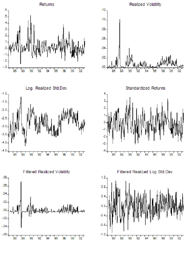
One of the prominent features of model-free measures of volatility, especially at a higher fre-quency of observation, is their temporal persistence. Figure 1 plots all four series used in our analy-sis, V2

t ;Lt;Rt and Zt. The well-documented volatility clustering can be directly observed both in the realized volatility and the log-standard deviation series. This clustering suggests that there should be a certain degree of temporal correlation in both series, with the log-standard deviation to possibly exhibit stronger correlation.

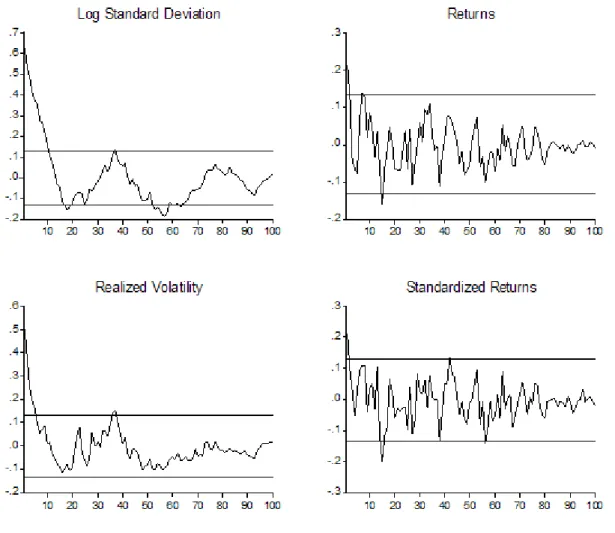
An initial gauging of the strength of serial correlation in the series is provided by the cor-relograms, that are presented in gure 2. The returns and the standardized returns have minimal memory, as the correlograms are within the their two standard error bounds, except for the autocor-relation of order one. The correlograms of the realized volatility and log-standard deviation series exhibit much larger correlation: the autocorrelations of the realized volatility series drop below their two standard error bounds at about lag 5 while the corresponding autocorrelations of the log-standard deviation series do the same at about lag 10. None of the descriptive signs of long memory

(8)

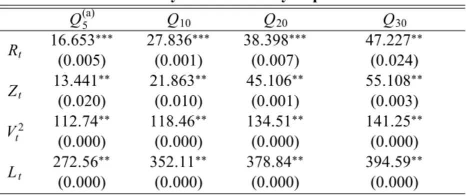
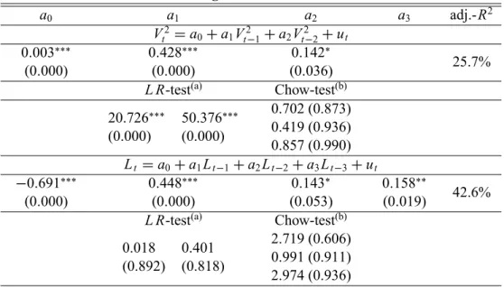
can be traced in the correlograms of the two volatility series; their autocorrelations die out very fast, a clear indication of short memory. Therefore, it appears that all four series can be treated as short-memory, covariance stationary processes.7 _{In table 1 we present results from the application of the} standard portmanteau test of Ljung and Box (Q-test). TheseQ-tests were performed for lags 5, 10, 20 and 30 and indicate the presence of various degrees of serial correlation. In agreement with the correlograms, the Q-tests show that the serial correlation is stronger in the volatility series that in the returns. For the analysis that follows we also use ltered versions of the realized volatility and log-standard deviation series, obtained from tting autoregressive models of orders 2 and 3 respec-tively - estimation results are given in table 3.8 _{We denote these two series by} _Vf

t and Ltf. With the ltered (residual) series we can work with the non-predictable (from its own past) component of realized volatility.

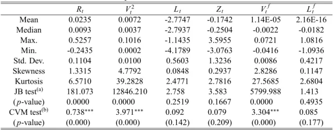
In table 2 we present descriptive and distributional statistics for all six series, that is including the ltered versions noted above. Given that the series appear to only have short (or no) memory, we can use standard distributional tests to examine whether they conform to an underlying Gaussian distribution. We use two distributional tests for gauging normality, the sample moments-based test of Jarque and Bera (1982) and the sample quantiles-based Crámer-Von Mises test. The tests are in agreement that, as expected, the returns and the realized volatility series have large deviations from normality while the standardized returns and the log-standard deviation series (including the ltered seriesLtf) appear to be coming from an underlying Gaussian distribution. In the next session, where we present our results for the linkages between volatility and returns, we mainly use the log-standard deviation as our measure of volatility.

Summarizing, our ndings appear to be consistent with the rest of the literature: nearly un-correlated and non-normal returns, serially un-correlated and non-normal realized volatility, serially correlated and normal realized log-standard deviation and normal standardized returns. The only 7_{Also note that the sample size we have available is relatively small for computing accurate estimates of the long} memory parameter (fractional order) of the series.

8_{In table 3 and all subsequent tables with estimation results we present also the results from (a) Chow}_F_{-type tests for} structural stability for two breakpoints (individually and jointly) April 1995 (market liberalization/full capital mobility) and October 1999 (global peak of the ASE index), and (b) Ramsey's RESET test for functional form speci cation. As expected, the regression models using the realized volatility do not pass the RESET test whereas the robust regression models with the log-standard deviations do pass the test; this clearly shows the effect of the double stabilizing transfor-mation of the square root and the logarithm

(9)

difference with the recent realized volatility difference is the lower degree of temporal dependence that we nd in the realized volatility series: our series have short rather than long memory.

IV. Tests on Asymmetric Volatility

This section empirically examines the asymmetric relationship between future logarithmic real-ized standard deviation and past standardreal-ized A.S.E. market returns and past log realreal-ized volatility from February 1985 to June 2003. In order to identify the channels of asymmetry between risk and return and the asymmetries in temporal dependencies in volatility we start by estimating simple regressions gauging the, so-called, volatility feedback effect - that is, the contemporaneous relation-ship between risk and return. The volatility feedback regressions take the same form as in Bollerslev and Zhou (2005), that is:

Rt DaC XtCut; (6)

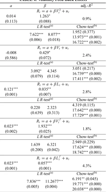
for the various realized risk measures Xt described in the previous section, namely the realized volatilityV2

t , the realized standard deviationVt, the logarithmic standard deviation Lt, the ltered realized volatilityV_tf and the ltered realized log standard deviationL_tf. The results on the volatil-ity feedback effect are given in table 4 and are all consistent with the potential presence of some positive feedback between realized risk and returns: while the regression t is less than 5% in all ve cases, the estimated coef cients appear to be statistically signi cant. The positive signs from these regressions are what is conventionally found and anticipated. Note that all the regressions except for the rst (realized volatility) and the last ( ltered log-standard deviation) pass the RESET test for functional form speci cation as well as the breakpoint test for April 1994, while they fail (as one would expect) to pass the breakpoint test for October 1999 where we have the global peak of the index.

In examining the possible presence of “leverage” in our data we employ the following generic regression:

a.B/vt Da0C rt 1C rt 1 irt.rt 1<0/Cut (7)

(10)

vt stands for any of the four measures of realized volatilityVt2;Lt;Vtf;Ltf.

rt stands for any of the two measures of returns Rt orZt.

a.B/is an autoregressive polynomial of degree 0 (ifvt DVtf orLtf), 2 (ifvt DVt2) or 3 (if

vt D Lt), whereBis the backward shift operator Bjxt Dxt j,

irt stands for the indicator function that takes the value of one when past period's returns (as de ned byrt) are negative.

the coef cients and measure the possible presence of a leverage/asymmetric effect: such a presence is related to an ex-ante anticipation for a parametric inequalities of the form _C <

0 and < _{j j}. The tables with the results also include a Wald-type hypothesis test for the null ofH0 C D0.

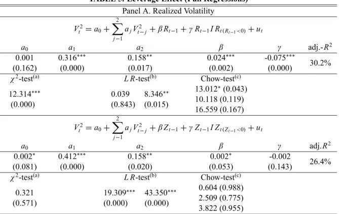
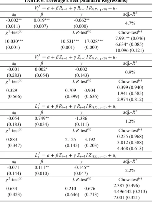
Our results for these leverage effect regressions are give in tables 5 and 6. The estimation results are statistically robust and economically consistent with the presence of strong asymmetries between risk and return in the A.S.E. market. The inclusion of lagged returns and their asymmetry indicator does not really affect the strong positive relationship between past and current risk - note that the estimates of thea.B/ parameters do not really change with respect to the corresponding estimates in table 3 and all remain signi cant. In six out of eight possible regressions (using all measures of risk and return noted above) we nd statistically signi cant estimates for the leverage parameters and with the anticipated signs and relative magnitudes. In four out of these eight possible regressions we also nd that the leverage estimates for are not only negative and larger (in absolute value) than the estimates for but also that the estimates for _C (measuring the total effect of negative returns) were larger than the estimates for alone (measuring the effect of positive returns). We note that it appears that the use of the standardized returns clouds the presence of the leverage effect: the regressions using the (simple) returns reveal the leverage effect much more strongly. Finally, it appears that almost all speci cations are well speci ed, as they pass both the RESET speci cation test and the Chow tests for three different break periods.

The interpretation of these results is actually quite interesting, when viewed in the context of a small and relatively inef cient market as the A.S.E.: negative lagged returns imply a stronger

(11)

and negative response of current volatility, when compared to the weaker and positive response of current volatility to positive lagged returns. Let us consider as an example one of the estimated regressions, the regression of realized volatility on past returns in table 5 (panel A): the response estimate for positive returns is 0.024 while the response estimate for negative returns is 0.024-0.075=-0.051. This implies that a 1% increase in the monthly A.S.E. returns will increase average monthly volatility by 0.024 when the market keeps rising; on the other hand, a 1% reduction in the returns will increase average monthly volatility by 0.051 when the market keeps falling.

The combined results from the volatility feedback regressions and the leverage regressions are strong indications that the A.S.E. market behaves like a “textbook” case, following well-established nancial rules: not only there is strong evidence of nancial leverage, but there appears that the A.S.E. market has a time-varying risk premium that is an increasing function of volatility; that premium increases with an anticipated increase in volatility thus raising the anticipated return on equity, which in turn implies an immediate decline on equity price. Could these results imply that our realized volatility measure could be used as a signi cantly priced factor in the A.S.E. returns? If yes, how would this result compare with the related existing literature? We explore these questions in the following section.

V. Realized Volatility as a Priced Factor in A.S.E. Returns

In this section we turn in examining whether contemporaneous and long-term measured market realized risk could be a priced factor in A.S.E. common stock returns. Time-varying aggregate real-ized market volatility implies changes in the set of future investment opportunities for the long-term investor (see, for example, Chen (2003) and Ang, Hodrick, Xing and Zhang (2005)). In an uncon-ditional multi-factor asset pricing framework similar to Merton (1973) and Campbell (1996) we ask whether realized volatility is such a factor and as a result whether differences in the unconditional premia across A.S.E. portfolios should be related to differences in their unconditional exposures to aggregate market volatility.

In order to establish a connection between portfolio risk premia and aggregate realized volatil-ity V2

(12)

pricing model with a beta-premium representation, where betas with different measures of realized risk serve as competing factors in average returns on stock portfolios from the A.S.E.:

E Re_i D 0C m imC V O L i V O LC S M B i S M BC H M L i H M L; (8)

whereRe

i;t D Ri;t Rf;t is the simple excess return on asseti, 's are the portfolios' factor loadings (betas), S M B and H M L are the two Fama-French (1993) size and book-to-market related factor mimicking portfolios, respectively, V O Lt is the aggregate realized volatility factor (V O Lt D Vt2 orLt), 's are the prices of beta risk and 0is the pricing error (the difference between actual and implied average returns). The inclusion of the two size and value Fama-French portfolios enables to ask whether realized risk has any marginal explanatory power for the cross-section of A.S.E. returns over and above any aggregate size and value effects captured byS M B andH M L.

The linear relationship between aggregate realized risk and average portfolio returns in (8) is empirically examined using the three-step Fama-MacBeth (1973) methodology. In the rst step, and for each portfolioi D1; :::;N, the unconditional betas are estimated from time-series regressions of

simple realized portfolio returnsRi on the market returnRm, realized risk (realized market variance

V2_{and realized logarithmic market standard deviation}_L_{, respectively) and two Fama-French (1993)} zero-cost size and value factor-mimicking portfoliosS M B andH M L, respectively:9

Ri;t D 0C imRm;tC i V O LV O LtC i S M BS M BtC i H M LH M Lt Cui;tI 8i D1; :::;N (9)

In the second step, the unconditional prices of beta risk ( 's ) are estimated by running a set monthly

(t _D1; :::;T) cross-sectional OLS regressions of realized portfolio excess returns (Re

t) on the esti-mated betas:

Re

t D 0C mbimC V O Lbi V O LC S M Bbi S M BC H M Lbi H M LCetI 8t D1; :::;T (10)

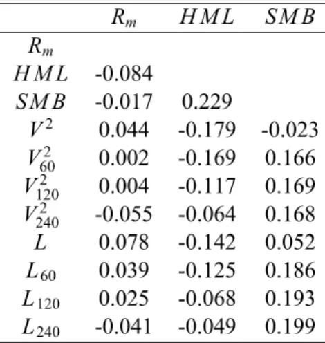
Equation (10) has been estimated using betas with both contemporaneous and long-term (60-day, 9_{Table 9 reports the sample correlation matrix of the factors used in the cross-sectional asset pricing tests. The low} estimated correlation coef cients indicated that the factors can be used as independent sources of risk and thus portfolio betas can be estimated from the multivariate regression of returns on the factors in (9).

(13)

120-day and 240-dayV2_and_L_{) realized market volatilities.}10

In the nal step, we estimate and we infer about the beta prices of risk ( s) and the pricing error term ( ₀, the difference between the actual and tted values in (10)) using the time-series estimates of the cross-sectional regression estimates and the Shanken's (1992) correction for the fact that betas were estimated with error from the rst-step regression in (9).

A. Portfolio Construction and Data Description

In what follows we use monthly observations from A.S.E. and we employ a variant of the Fama and French (1993) methodology to construct returns on 25 rm-characteristic single-sorted portfolios on book-to-market, size, dividend-yield, price-earnings and 3-month momentum, and the two size and book-to-market factor mimicking portfolios, Small-Minus-Big (S M B) and High-Minus-Low (H M L) respectively. Our portfolio formation approach slightly differs from Fama-French (1993) and closely follows Lewellen (1999) in the sense that we construct monthly dynamic investment strategies where portfolio rebalancing takes place at the beginning of each month using the most current history of portfolio returns and asset characteristics.11

The 25 portfolios were constructed using last month's accounting and nancial data. First, we break the full menu of A.S.E. common stocks available at any given montht into 5 groups (based on accounting information) each containing an equal number of stocks and second, we compute the simple market capitalization weighted-average monthly holding period return for each of the 5 portfolios fromttot_C1. The procedure is repeated every month from July 1991 to June 2003 and we end up with time-series data of simple returns on each characteristics-sorted portfolio. For the construction of excess returns we use the average T-bill rate.

For the value factor portfolio H M Lwe use the Fama and French (1993) 40-20-40 rule. How-ever, for the S M B portfolio, we adjust the formation mechanism to account for peculiarities of the Greek data. We use the 70th quantile of the market value instead of the median that was used by Fama and French (see also Dimson et al. (2003)). Using a larger breakpoint we can

10_{The long-term realized volatilities were computed using the corresponding rolling sample squared returns.}

11_{We have also estimated the beta prices of risk using portfolio returns employing a 6-month rebalancing. However,} there is no quantitatively important differences in our results.

(14)

create a distribution of the market value similar to that of Fama and French, while the small capitalization portfolio represents on average the 8% of the total A.S.E. market. At the end of June of each year, we create the size and book-to-market double-sorted portfolios of Fama and French (1993) (SL;S M;S H;B L;B M and B H) and calculate the value-weighted monthly re-turns for the next 6 months. Then, the aggregate book-to-market and size portfolios are de ned as

H M L D.S HCB H/=2 .SLCB L/=2 andS M B D.SLCS MCS H/=3 .B LCB MCB H/=3

respectively.12

Panel A of Table 7 reports the descriptive statistics of the value weighted S M B and H M L

portfolios and Panel B reports the full-sample statistical characteristics for the 25 portfolios with “diff.” denoting the difference in simple returns between the extreme cells. The internationally documented “size” premium of small-cap over large-cap stocks (Fama and French (1998)) appears to be a fact for A.S.E. also. The size zero-cost factor portfolio S M B delivers a 1.18% monthly premium and the difference between the extreme small-cap portfolio and large-cap portfolios is 2.39% per month. Our data set reveals also a value premium for A.S.E. stocks from 1991 to 2003, although smaller then the size effect. The monthly sample average return forH M Lis 0.6% whereas the premium of the value portfolio over the growth portfolio is 2% per month.

Our A.S.E. data yield a relative premium for the high dividend-yield and low price-earnings ratio portfolios. The difference between the high and low D/Y portfolio is 1.36% per month and the difference between the lowest and the highest P/E portfolio is 1.46%. Finally, and as was naturally expected, winners deliver an average premium of 1.17% per month over losers.

B. The Cross-Section of Returns and Market, Value, Size and Realized Volatility Risks

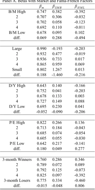
Panel A of Table 8 reports the full-sample estimates of factor loadings on market returns ( _m), on the two Fama-French aggregate size and value factors ( _{S M B} and _{H M L}), whereas Panel B illustrates the estimated loadings on the different horizon measures of realized risk (60-day, 120-day and 240-120-day _V2and _L, respectively). Consistent with the international literature our estimates

12_{We use data from 1991 since the low number of stocks in the late 1980s does not enable us to form the 6 size-B/M} Fama-French portfolios with a considerable number of stocks within each group. Statistics for the six Fama-French portfolios are available upon request.

(15)

of market betas show a low spread across portfolios indicating a relatively at relationship between market loadings and the cross-section of average stock returns. In contrast, the spread in betas for the Fama-French factors are large and with the correct sign both for the value and size portfolios. The difference in _{S M B} between the value and growth portfolio is 0.288 and the difference between the betas in smallest and largest portfolio is 1.460. Similarly, the cross-sectional difference in _{H M L} for value and growth stocks is 0.494 whereas for small-cap and large-cap stocks is 0.216. Our ndings support the view of Fama and French (1993) that small and growth stocks are more risky and carry a premium for their exposure to economy-wide value and size factors. Finally, and for the 15 D/Y, P/E and momentum portfolios we observe low spreads in the estimated market and

S M Bbetas. However, there exist economically signi cant differences in the estimated loadings for the aggregate value mimicking factor H M L (-0.206, 0.277 and 0.806 respectively) in favor of an aggregate value risk factor in A.S.E. returns.

Loadings on realized market variance and logarithmic market standard deviation are shown in Panel B of Table 8. Value portfolios appear to have much higher sensitivities with realized risk than growth stocks and the difference between the extreme portfolios is 0.938 for contemporaneous realized volatility and 0.024 for the contemporaneous realized log standard deviation. Also, there exist considerable spreads for the long-horizon de ned measures of realized risk although the levels and therefore the differences in the estimated betas are smaller that their contemporaneous coun-terpart. Our estimation results deliver also a positive difference between the long-term volatility factor loadings for the small-large, low-high D/Y and winners-losers portfolios. However, while the contemporaneous correlation of these zero-cost portfolios with aggregate volatility is negative the estimates become positive when realized risk is measured over longer periods.

Table 10 illustrates the results from the cross-sectional regressions in (10) of excess portfolio returns on the estimated factor loadings on Rm,S M B, H M Land realized volatility.13 For each re-gression we report the estimate of each coef cient, the standard error and the average adj-R2_{of the} regressions. The rst row of Panel A reports the results for the static single-factor CAPM. Our data provide further evidence in the international literature about the failure of the CAPM. The model 13_{Also, and in order to identify asymmetries in the relationship between realized risk and average returns, and the} pricing of downside risk, we follow Ang, Chen and Xing (2004) and we estimate regressions of average excess portfolio returns on downside betas. However, our results cannot provide evidence for any downside risk pricing in A.S.E. These results are available upon request.

(16)

delivers a highly insigni cant market risk premium which indicates a at relationship between mar-ket betas and average excess portfolio returns. Although, the singleV2_{factor is not priced when} used alone, it is highly signi cant (1% level) in the long-horizon regressions, the estimated beta prices are quite stable in all speci cations ranging from 0.0228 for the 60-day regression to 0.385 in the 240-day regression respectively and it captures almost a third of the cross-sectional variation in average excess returns. Our results appear to be consistent with the hypothesis that the exposure to aggregate realized market risk is priced in the cross-section of A.S.E. portfolio returns.

The inclusion of H M LandS M B betas in the cross-sectional regression improves the explana-tory performance of (10) and the adj.-R2 _{increases close to 60% for all horizon speci cations. In} this full speci cation the V2 _{coef cient becomes smaller in magnitude ranging from 0.0052 to} 0.0406 exhibiting a strict monotonic pattern as the horizon increases but it loses some of its sta-tistical signi cance. The premium for the size factor S M B is positive and highly signi cant for the contemporaneous and 60-day regression while its signi cance falls with when longer horizon realized volatility betas are included. However, the estimates are quite stable across speci cations. The H M L factor delivers negative and small in magnitude premia in all regressions and they are signi cant at only a 10% level. These results indicate that our search for a realized market variance risk factor that could be a priced in A.S.E. returns is independent of any market, size or value risk effects.

The results for the cross-sectional regressions for the logarithmic market realized standard devi-ation in Panel B are even more clear since theL- factor appears to better priced both in the contem-poraneous and the long-horizon speci cation of (10). When it used alone, it increases the explained cross-sectional variation of average returns to 21% with a highly signi cant 0.3789 price of beta risk for the contemporaneous risk speci cation, and adj.-R2_{increases to 40% in long-horizon setting.} The pricing errors are signi cant indicating that other factors may be important for the cross-section of returns. When we include the Fama-French factors the beta market price of risk _mbecomes posi-tive but it is still insigni cant whereas price of realized log standard deviation beta risk is signi cant at a 5% level with stable values of 0.2972, 0.2950, 0.2539 and 0.2182 for the contemporaneous, 60-day, 120-day and 240-day regressions respectively, and the explained cross-sectional variation in returns increases to 60%. The statistical signi cance and the stability of the size factor premia

(17)

S M B in all regressions indicate that there exist size effects in A.S.E. that are unrelated to risks associated with realized volatility (premia range from 0.0102 to 0.0150). However, and as in the realized volatility case in panel A, the prices of risk for the value factor are small, negative and signi cant only at a 10% level and as a result we cannot infer about the economic importance of aggregate book-to-market mimicking factor to capture any of the cross-sectional variation in A.S.E. returns.

Overall, our results can be easily summarized. There is a clear positive linear relationship be-tween average portfolio returns and loadings on realized aggregate volatility (either realized volatil-ity or logarithmic standard deviation), and, further, this relationship is independent of any mar-ket, size or book-to-market effects as these are captured by the three-factor Fama-French (1993) model. The spread in full-sample (1991-2003) estimated betas with both contemporaneous and long-horizon (60-day, 120-day and 240-day) realized risk capture a large part of the cross-sectional variation in A.S.E. returns and generate large in magnitude and statistically signi cant premia. How-ever, there is clear space for the Fama-French aggregate size factorS M Bbut we cannot safely infer about the importance of the aggregate value factorH M Lwhen realized market risk is considered.

VI. Concluding Remarks

Using a newly developed data set of daily, value-weighted stock returns from the Greek stock market, we construct and analyze the properties of the monthly realized volatility of the Athens Stock Exchange (A.S.E.) from 1985 to 2003. Our work is related to two lines of the volatility literature: the rst is the line that deals with the construction and properties of model-free measures of volatility and the second, is the line that examines the, so-called, “leverage effect”. We nd that the realized volatility series exhibits short memory and its distribution is not Gaussian while the realized log standard deviation series exhibit short memory but probably has an underlying Gaussian distribution. These results are conformable with the existing literature. We also nd evidence in favor of the presence of volatility feedback effects and asymmetries between lagged returns and volatility: not only there is strong evidence of nancial leverage, but there appears that the A.S.E. market has a time-varying risk premium that is an increasing function of volatility.

(18)

In addition to this we ask whether the various de nitions of market realized risk can serve as competing aggregate risk factors, in an unconditional asset pricing model, that could explain the cross-sectional variation in average returns on rm-characteristic single-sorted portfolios. Our re-sults indicate a clear positive linear relationship between loadings (betas) on realized aggregate volatility (either realized volatility or logarithmic standard deviation) and this relationship is in-dependent of any market, size or book-to-market effects as these are captured by the three-factor Fama-French (1993) model.

The high explanatory power of realized risk in the asset pricing tests indicates that there should be a link between realized risk and macroeconomic conditions; a potential extension of our research, using the computed realized volatility series, could be the examination of this association of realized market risk with the future state of the economy.

(19)

References

Andersen T. and T. Bollerslev. 1998. Answering the Skeptics: Yes, Standard Volatility Models Do Provide Accurate Forecasts. International Economic Review 39: 885-905.

Andersen, T.; Bollerslev, T.; Diebold, F.; and Labys, P. 2001a. The Distribution of Exchange Rate Volatility. Journal of the American Statistical Association 96: 42-55.

Andersen, T.G.; Bollerslev, T.; Diebold, F.X.; and Labys, P. 2001b. Modelling and Forecast-ing Realized Volatility. NBER workForecast-ing paper no. 8160. Cambridge, Mass.: National Bureau of Economic Research.

Andersen, T.G.; Bollerslev, T.; Diebold, F.X.; and Labys, P. 2001c. The Distribution of Stock Return Volatility. Journal of Financial Economics 61: 43-76.

Ang, A.; Chen, J.; and Xing, Y. 2004. Downside Risk. Columbia University, unpublished monograph.

Ang, A.; Hodrick, R.; Xing Y.; and Zhang, X. 2005. The cross-Section of Volatility and Ex-pected Returns. Journal of Finance: forthcoming.

Barkoulas, J.; Baum, Ch.; and Travlos, N. 2000. Long Memory in the Greek Stock Market. Applied Financial Economics 10: vol. 2.

Barndorff-Nielsen, O.; and Shephard N. 2001a. Non-Gaussian Ornstein-Uhlenbeck Based Mod-els and Some of their Uses in Financial Economics. Journal of the Royal Statistical Society: Series B, 63: 167–241.

Barndorff-Nielsen, O.; and Shephard N. 2001b. How Accurate is the Asymptotic Approxima-tion to the DistribuApproxima-tion of the Realized Volatility. mimeo.

Bekaert, G.; and Wu, G. 2000. Asymmetric Volatility and Risk in Equity Markets. Review of Financial Studies 13: 1-42.

Bollerslev, T.; and Zhou, H. 2005. Volatility Puzzles: A Simple Framework for Gauging Return-Volatility Regressions. Journal of Econometrics: forthcoming.

Campbell, J. 1996. Understanding Risk and Return. Journal of Political Economy 104: 298-345. Campbell, J.; and Hentschel, L. 1992. No News is Good News: An Asymmetric Model of Changing Volatility in Stock Returns. Journal of Financial Economics 31: 281-318.

Campbell, J.; Lettau, M.; Malkiel, B.G.; and Xu, Y. 2001. Have Individual Stocks Become More Volatile? An Empirical Exploration of Idiosyncratic Risk. Journal of Finance 56: 1 –43.

Chen, J. 2003. Intertemporal CAPM and the Cross-Section of Stock Returns. University of Southern California, unpublished monograph.

Dimson, E.; Nagel, S.; and Quigley, G. 2003. Capturing the Value Premium in the U.K. 1955-2001. Financial Analysts Journal : Vol 59, 6: 35-45

Engle, R.; and Ng, V.. 1993. Measuring and Testing the Impact of News on Volatility. Journal of Finance 48: 1749-1778.

Fama, E.; and MacBeth J. 1973. Risk, Return and Equilibrium: Empirical Tests. Journal of Political Economy 71: 607-636.

(20)

Fama, E.; and French, K. 1993. Common Risk Factors in the Returns on Stocks and Bonds. Journal of Financial Economics 33: 3-56.

Fama, E.; and French, K. 1998. Value versus Growth: The International Evidence. Journal of Finance 53: 1975-2000.

French, K.; Schwert, G.; and Stambaugh, R. 1987. Expected Stock Returns and Volatility. Journal of Financial Economics 19: 3-30.

Lewellen, J. 1999. The Time-Series Relations Among Expected Return, Risk, and Book-to-Market. Journal of Financial Economics 54: 5-43.

Merton, R. 1973. An Intertemporal Capital Asset Pricing Model. Econometrica 41: 867-887. Merton, R. 1980. On Estimating the Expected Return on the Market: An Exploratory Investiga-tion. Journal of Financial Economics 8: 323-361.

Nelson, D. 1991. Conditional Heteroskedasticity in Asset Returns: A New Approach. Econo-metrica 59: 347-370.

Poterba, J.; Summers L. 1986. The Persistence of Volatility and Stock Market Fluctuations. American Economic Review 76: 1142-1151.

Pindyck, R.S. 1984. Risk, In ation, and the Stock Market. American Economic Review 74: 334–351.

Schwert, G. 1990. Stock Market Volatility. Financial Analysts Journal: May-June: 23-34. Shanken, J. 1992. On the Estimation of Beta-Pricing Models. Review of Financial Studies 5: 1-33.

Travlos, N. 1992. Athens Stock Exchange: Creation of a Stock Data Bank and Risk-Returns Characteristics for the Period 1981-1990. University of Piraeus, unpublished monograph.

(21)

(22)

(23)

TABLE 1. Dynamic Volatility Dependence Q(a)₅ Q10 Q20 Q30 Rt 16:653 .0:005/ 27:836 .0:001/ 38:398 .0:007/ 47:227 .0:024/ Zt 13:441 .0:020/ 21:863 .0:010/ 45:106 .0:001/ 55:108 .0:003/ V2 t 112:74 .0:000/ 118:46 .0:000/ 134:51 .0:000/ 141:25 .0:000/ Lt 272:56 .0:000/ 352:11 .0:000/ 378:84 .0:000/ 394:59 .0:000/ (a)_Q

kis Ljung-Box test for autocorrelation fork D5;10;20;30 lags.

(24)

TABLE 2. Descriptive Statistics of Returns and Volatilities

Rt Vt2 Lt Zt Vtf Ltf

Mean 0.0235 0.0072 -2.7747 -0.1742 1.14E-05 2.16E-16

Median 0.0093 0.0037 -2.7937 -0.2504 -0.0022 -0.0182 Max. 0.5257 0.1016 -1.1435 3.5955 0.0721 1.0816 Min. -0.2435 0.0002 -4.1789 -3.0763 -0.0416 -1.0936 Std. Dev. 0.1104 0.0100 0.5603 1.3236 0.0086 0.4217 Skewness 1.3315 4.7792 0.0848 0.2937 2.8286 0.1147 Kurtosis 6.5710 39.2828 2.4771 2.7816 27.5685 2.6804 JB test(a) (p-value) 181.073 0.0000 12846.210 0.0000 2.758 0.2519 3.583 0.1667 5799.988 0.0000 1.413 0.4935 CVM test(b) (p-value) 0.738 (0.000) 3.971 (0.000) 0.092 (0.142) 0.079 (0.209) 3.304 (0.000) 0.085 (0.177) (a)_{Jarque-Bera normality test.}

(b)_{Crámer-Von Mises normality test.}

(25)

TABLE 3. Autoregressive Estimation:V2_and _L a0 a1 a2 a3 adj.-R2 V2 t Da0Ca1Vt21Ca2Vt22Cut 0:003 .0:000/ 0:428 .0:000/ 0:142 .0:036/ 25.7%

L R-test(a) _Chow-test(b) 20.726 50.376 (0.000) (0.000) 0.702 (0.873) 0.419 (0.936) 0.857 (0.990) Lt Da0Ca1Lt 1Ca2Lt 2Ca3Lt 3Cut 0:691 .0:000/ 0:448 .0:000/ 0:143 .0:053/ 0:158 .0:019/ 42.6%

L R-test(a) _Chow-test(b) 0.018 0.401

(0.892) (0.818)

2.719 (0.606) 0.991 (0.911) 2.974 (0.936)

(a)_{Log likelihood ratio value (}_p_{-value) of Ramsey RESET Test with one and two tted terms.} (b)_{Chow test (}_p_{-value) of structural change: 1994:5, 1999:10, and both.}

(26)

TABLE 4. Volatility Feed-Back Effects a adj.-R2 Rt DaC Vt2Cut 0.014 (0.113) 1.263 (0.088) 0.9%

L R-test(a) _Chow-test(b)

7.622 8.077 (0.006) (0.018) 1.952 (0.377) 13.973 (0.001) 16.722 (0.002) Rt DaC Vt Cut -0.008 (0.586) 0.429 (0.072) 2.4%

L R-test(a) _Chow-test(b) 3.092 4.345 (0.079) (0.114) 3.051 (0.217) 16.739 (0.000) 17.411 (0.002) Rt DaC Lt Cut 0.121 (0.001) 0.035 (0.007) 2.8%

L R-test(a) _Chow-test(b) 0.220 2.323 (0.639) (0.313) 4.319 (0.115) 17.642 (0.000) 17.729 (0.001) Rt DaC Vtf Cut 0.023 (0.002) 1.932 (0.025) 1.8%

L R-test(a) _Chow-test(b) 1.639 6.321 (0.200) (0.042) 2.949 (0.229) 17.624 (0.000) 18.742 (0.001) Rt DaC Ltf Cut 0.023 (0.001) 0.057 (0.001) 4.3%

L R-test(a) _Chow-test(b) 7.836 11.2677

(0.005) (0.004)

6.191 (0.045) 19.771 (0.000) 20.038 (0.000)

(a)_{Log likelihood ratio value (}_p_{-value) of Ramsey RESET Test with one and two tted terms.} (b)_{Chow test (}_p_{-value) of structural change: 1994:5, 1999:10, and both.}

(27)

TABLE 5. Leverage Effect (Full Regressions)

Panel A. Realized Volatility

V2 t Da0C 2 X j 1 ajVt j2 C Rt 1C Rt 1I Rt.Rt 1<0/Cut a0 a1 a2 adj.-R2 0.001 (0.162) 0.316 (0.000) 0.158 (0.017) 0.024 (0.002) -0.075 (0.000) 30.2%

2_-test(a) _{L R}_-test(b) _Chow-test(c)

12.314 (0.000) 0.039 8.346 (0.843) (0.015) 13.012 (0.043) 10.118 (0.119) 16.559 (0.167) V2 t Da0C 2 X j 1 ajVt j2 C Zt 1C Zt 1I Zt.Zt 1<0/Cut a0 a1 a2 adj.R2 0.002 (0.081) 0.412 (0.000) 0.158 (0.020) 0.002 (0.053) -0.002 (0.143) 26.4%

0.321 (0.571) 19.309 43.350 (0.000) (0.000) 0.604 (0.988) 2.509 (0.775) 3.822 (0.955) (a)_{Wald test (}_p_{-value) for}_H

0 C D0.

(b),_{Log likelihood ratio value (}_p_{-value) of Ramsey RESET Test with one and two tted term} (c)_{Chow test (}_p_{-value) of structural change: 1994:5, 1999:10, and both.}

(28)

Panel B. Realized Log Standard Deviation Lt Da0C 3 X j 1 ajLt jC Rt 1C Rt 1I Rt.Rt 1<0/Cut a0 a1 a2 a3 adj.-R2 -0.961 (0.000) 0.356 (0.000) 0.170 (0.021) 0.154 (0.021) 1.021 (0.013) -2.081 (0.042) 43.7%

1.972 (0.160) 0.434 1.132 (0.509) (0.568) 3.437 (0.752) 4.221 (0.647) 9.182 (0.687) Lt Da0C 3 X j 1 ajLt j C Zt 1C Zt 1I Zt.Zt 1<0/Cut a0 a1 a2 a3 adj.-R2 -0.807 (0.000) 0.409 (0.000) 0.177 (0.018) 0.149 (0.026) 0.117 (0.009) -0.151 (0.044) 43.9%

0 C D0.

(b)_{Log likelihood ratio value (}_p_{-value) of Ramsey RESET Test with one and two tted terms} (c)_{Chow test (}_p_{-value) of structural change: 1994:5, 1999:10, and both.}

(29)

TABLE 6. Leverage Effect (Standard Regressions) Vtf DaC Rt 1C Rt 1I Rt.Rt 1<0/Cut a0 adj.-R2 -0.002 (0.011) 0.019 (0.007) -0.062 (0.000) 4.7%

10.030 (0.001) 10.531 17.028 (0.001) (0.000) 7.991 (0.046) 6.634 (0.085) 10.096 (0.121) V_tf _Da_C Zt 1C Zt 1I Zt.Zt 1<0/Cut a0 adj.-R2 -0.001 (0.283) 0.002 (0.054) -0.002 (0.143) 0.9%

0.329 (0.566) 0.709 0.904 (0.399) (0.636) 0.399 (0.940) 1.941 (0.585) 2.974 (0.812) L_tf _Da_C Rt 1C Rt 1I Rt.Rt 1<0/Cut a0 adj.-R2 -0.054 (0.183) 0.749 (0.034) -1.386 (0.111) 1.2%

0.883 (0.347) 2.125 3.192 (0.145) (0.203) 0.255 (0.968) 3.012 (0.388) 4.468 (0.613) Ltf DaC Zt 1C Zt 1I Zt.Zt 1<0/Cut a0 adj.-R2 -0.071 (0.144) 0.111 (0.010) -0.145 (0.047) 2.2%

0 C D0.

(b)_{Log likelihood ratio value (}_p_{-value) of Ramsey RESET Test with one and two tted terms.} (c)_{Chow test (}_p_{-value) of structural change: 1994:5, 1999:10, and both.}

(30)

TABLE 7. Statistics for SMB, HML and 25 Book-to-Market, Size, Dividend-Yield, Price-Earnings and 3-month Momentum Single Sorted Portfolios

Panel A. SMB and HML S M B H M L Mean 0.0118 0.0060 Median -0.0031 0.0071 Maximum 0.3270 0.2851 Minimum -0.2636 -0.2776 Std. Dev. 0.0789 0.0749 Skewness 0.7866 -0.0914 Kurtosis 5.7579 6.4002 Jarque-Bera 65.5271 75.3675 Prob. 0.0000 0.0000 Panel B. B/M Portfolios

High 2 3 4 Low diff.

Mean 0.0211 0.0141 0.0073 0.0067 0.0111 -0.0100 Median 0.0008 -0.0049 -0.0007 0.0088 0.0051 Maximum 0.3987 0.4400 0.3366 0.4052 0.3922 Minimum -0.2948 -0.2181 -0.1938 -0.2573 -0.2025 Std. Dev. 0.1176 0.1052 0.0994 0.0967 0.0958 Skewness 0.7933 0.9791 0.6255 0.5175 0.6906 Kurtosis 4.2631 4.6063 3.6971 4.9967 5.1804 Jarque-Bera 24.6758 38.4873 12.3048 30.3493 39.9722 Prob. 0.0000 0.0000 0.0021 0.0000 0.0000

Panel C. Size Portfolios

Large 2 3 4 Small diff.

Mean 0.0109 0.0105 0.0147 0.0241 0.0348 0.0239 Median 0.0101 0.0039 0.0006 0.0031 0.0034 Maximum 0.4294 0.4530 0.5907 0.5147 0.5998 Minimum -0.1976 -0.2762 -0.2758 -0.2930 -0.3073 Std. Dev. 0.0904 0.1079 0.1226 0.1333 0.1535 Skewness 0.8296 0.6555 0.9461 0.8805 1.2641 Kurtosis 5.8419 4.6370 5.8077 4.8910 5.4570 Jarque-Bera 64.9771 26.3925 68.7814 40.0650 74.5722 Prob. 0.0000 0.0000 0.0000 0.0000 0.0000

(31)

Panel D. Dividend-Yield Portfolios

Panel E. Price-Earnings Portfolios

Mean 0.0079 0.0081 0.0091 0.0125 0.0225 0.0146 Median 0.0017 0.0091 -0.0015 0.0029 0.0139 Maximum 0.4526 0.3915 0.4031 0.2869 0.3518 Minimum -0.2556 -0.2032 -0.2526 -0.2197 -0.1558 Std. Dev. 0.1167 0.1004 0.0967 0.0881 0.0988 Skewness 0.9835 0.4218 0.7230 0.4778 0.7690 Kurtosis 5.6917 3.9484 5.3587 3.6723 3.5172 Jarque-Bera 66.6869 9.6658 45.9256 8.1902 15.7985 Prob. 0.0000 0.0080 0.0000 0.0167 0.0004

Panel F. 3-Month Momentum Portfolios

Winners 2 3 4 Losers diff.

(32)

TABLE 8. Betas for 25 Book-to-Market, Size, Dividend-Yield, Price-Earnings and 3-month Momentum Single Sorted Portfolios

Panel A. Betas with Market and Fama-French Factors m S M B H M L B/M High 0.747 0.382 -0.392 2 0.707 0.306 -0.032 3 0.702 0.058 -0.123 4 0.692 0.110 -0.011 B/M Low 0.678 0.095 0.102 diff. 0.069 0.288 -0.494 Large 0.990 -0.193 -0.203 2 0.932 0.477 -0.019 3 0.936 0.733 0.017 4 0.865 0.959 0.069 Small 0.802 1.267 0.013 diff. 0.188 -1.460 -0.216 D/Y High 0.643 0.140 -0.166 2 0.752 0.041 -0.203 3 0.678 0.133 0.003 4 0.727 0.149 0.088 D/Y Low 0.695 0.230 0.041 diff. -0.052 -0.090 -0.206 P/E High 0.822 0.266 0.136 2 0.713 0.184 -0.043 3 0.685 0.074 -0.054 4 0.605 0.055 -0.030 P/E Low 0.642 0.217 -0.141 diff. 0.180 0.049 0.277 3-month Winners 0.760 0.286 0.346 2 0.789 0.072 0.089 3 0.792 0.125 -0.073 4 0.825 0.097 -0.392 3-month Losers 0.775 0.334 -0.460 diff. -0.015 -0.048 0.806

(33)

Panel B. Betas with Realized Risk V2 _V2 60 V1202 V2402 L L60 L120 L240 B/M High 1.217 0.457 0.322 0.309 0.034 0.027 0.039 0.052 2 0.847 0.402 0.316 0.271 0.028 0.025 0.035 0.045 3 0.593 0.190 0.164 0.161 0.020 0.009 0.015 0.024 4 0.096 0.195 0.177 0.177 0.007 0.008 0.017 0.026 B/M Low 0.279 0.289 0.202 0.166 0.010 0.016 0.024 0.028 diff. 0.938 0.167 0.119 0.143 0.024 0.011 0.016 0.024 Large 1.757 0.383 0.368 0.313 0.030 0.022 0.032 0.045 2 1.093 0.533 0.543 0.462 0.027 0.031 0.052 0.070 3 0.629 0.490 0.497 0.440 0.021 0.029 0.049 0.065 4 0.404 0.555 0.530 0.471 0.023 0.034 0.054 0.070 Small 0.883 0.670 0.594 0.507 0.030 0.042 0.062 0.079 diff. 0.874 -0.287 -0.225 -0.194 0.000 -0.020 -0.030 -0.034 D/Y High 0.941 0.279 0.215 0.226 0.024 0.017 0.025 0.037 2 0.736 0.308 0.225 0.222 0.024 0.020 0.029 0.041 3 0.164 0.198 0.160 0.148 0.013 0.009 0.015 0.021 4 0.181 0.305 0.230 0.205 0.012 0.014 0.021 0.030 D/Y Low 0.515 0.309 0.261 0.237 0.016 0.018 0.028 0.038 diff. 0.426 -0.030 -0.047 -0.012 0.008 -0.001 -0.003 -0.001 P/E High 0.353 0.448 0.326 0.248 0.013 0.026 0.035 0.040 2 0.335 0.251 0.210 0.205 0.015 0.013 0.024 0.035 3 0.386 0.232 0.185 0.177 0.016 0.013 0.020 0.028 4 0.092 0.070 0.106 0.107 0.004 0.001 0.008 0.015 P/E Low 0.959 0.429 0.309 0.274 0.029 0.029 0.038 0.047 diff. -0.606 0.019 0.017 -0.026 -0.016 -0.003 -0.003 -0.007 3-month Winners -0.320 0.144 0.197 0.239 0.004 0.016 0.025 0.039 2 0.146 0.275 0.239 0.241 0.013 0.019 0.028 0.039 3 0.039 0.216 0.173 0.164 0.009 0.011 0.017 0.023 4 1.010 0.229 0.207 0.198 0.028 0.014 0.022 0.032 3-month Losers 0.119 -0.119 0.030 0.099 0.010 -0.007 0.004 0.011 diff. -0.439 0.264 0.167 0.139 -0.006 0.023 0.021 0.028

(34)

TABLE 9. Sample Correlation Matrix of Risk Factors Rm H M L S M B Rm H M L -0.084 S M B -0.017 0.229 V2 _0.044 _{-0.179 -0.023} V2 60 0.002 -0.169 0.166 V2 120 0.004 -0.117 0.169 V2 240 -0.055 -0.064 0.168 L 0.078 -0.142 0.052 L60 0.039 -0.125 0.186 L120 0.025 -0.068 0.193 L240 -0.041 -0.049 0.199

(35)

TABLE 10. Asset Pricing Cross-Sectional Regressions

Panel A. Realized Volatility

Factor/Premium _b₀ _b_m _b_V2 b_{S M B} b_{H M L} adj.-R2 Rm 0:0023 0:0065 3:4% (0.011)(a) _(0.0144) V2 ₀_:₀₀₀₄ ₀_:₀₀₄₁ ₃_:_99% (0.0020) (0.0029) 0:0045 7:84% (0.0018) V2_and_R m 0:0016 0:0017 0:0042 0:3% (0.0113) (0.0155) (0.0032) 0:0005 0:0041 3:95% (0.0028) (0.0030) V2_, _R m andF F 0:0115 0:0215 0:0052 0:0175 0:0004 60:26% (0.0073) (0.0104) (0.0029) (0.0029) (0.0059) 0:0056 0:0044 0:0164 59:33% (0.0021) (0.0019) (0.0029) V2 60 0:0045 0:0228 29:35% (0.0024) (0.0069) V2 60andRM 0:0051 0:0141 0:0264 29:71% (0.0093) (0.0133) (0.0077) V2 60,RM andF F 0:0087 0:0192 0:0137 0:0140 0:0091 58:61% (0.0072) (0.0103) (0.0072) (0.0036) (0.0051) V2 120 0:0050 0:0279 31:23% (0.0025) (0.0081) V2 120andRm 0:0150 0:0312 0:0414 41:46% (0.0092) (0.0139) (0.0096) V2 120,Rm;andF F 0:0133 0:0273 0:0231 0:0117 0:0098 58:64% (0.0079) (0.0125) (0.0122) (0.0043) (0.0052) V240 0:0071 0:0385 38:16% (0.0026) (0.0097) V240andRm 0:0157 0:0367 0:0588 53:39% (0.0081) (0.0126) (0.0109) V240,Rm;andF F 0:0145 0:0329 0:0406 0:0087 0:0097 62:9% (0.0074) (0.0123) (0.0162) (0.0046) (0.0049)

(a)_{Standard errors of estimates}

(36)

Panel B. Realized Logarithmic Standard Deviation Factor/Premium _b₀ _b_m _b_L _b_{S M B} _b_{H M L} adj.-R2 L 0:0044 0:3789 21:7% (0.0028)(a) _(0.1370) 0:1837 16:8% (0.0603) L andRm 0:0005 0:0071 0:4074 19:1% (0.0098) (0.0137) (0.1495) L, RmandF F 0:0074 0:0188 0:2972 0:0150 0:0005 61:5% (0.0069) (0.0097) (0.1287) (0.0032) (0.0059 L60 0:0047 0:3957 0 37:3% (0.0021) (0.1013) L60andRm 0:0067 0:0167 0:4633 39:5% (0.0087) (0.0124) (0.1114) L60, Rm andF F 0:0098 0:0218 0:2950 0:0125 0:0103 64:4% (0.0067) (0.0096) (0.1084) (0.0034) (0.0048) L120 0:0063 0:3081 41% (0.0024) (0.0733) L120andRm 0:0106 0:0259 0:4024 48:9% (0.0082) (0.0120) (0.0811) L120, RmandF F 0:0111 0:0253 0:2539 0:0104 0:0095 62:5% (0.0070) (0.0106) (0.1035) (0.0041) (0.0049) L240 0:0074 0:2550 40:6% (0.0026) (0.0611) L240andRm 0:0106 0:0285 0:3451 50:3% (0.0080) (0.0121) (0.0678) L240, RmandF F 0:0111 0:0267 0:2182 0:0102 0:0092 62:7% (0.0069) (0.0109) (0.0878) (0.0042) (0.0049)

(a)_{Standard errors of estimates}