Zurich Open Repository and Archive University of Zurich Main Library Strickhofstrasse 39 CH-8057 Zurich www.zora.uzh.ch Year: 2017
Delta networks for optimized recurrent network computation
Neil, D ; Lee, J-H ; Delbruck, T ; Liu, S-CAbstract: Many neural networks exhibit stability in their activation patterns over time in response to inputs from sensors operating under real-world conditions. By capitalizing on this property of natural signals, we propose a Recurrent Neural Network (RNN) architecture called a delta network in which each neuron transmits its value only when the change in its activation exceeds a threshold. The execu-tion of RNNs as delta networks is attractive because their states must be stored and fetched at every timestep, unlike in convolutional neural networks (CNNs). We show that a naive run-time delta net-work implementation offers modest improvements on the number of memory accesses and computes, but optimized training techniques confer higher accuracy at higher speedup. With these optimizations, we demonstrate a 9X reduction in cost with negligible loss of accuracy for the TIDIGITS audio digit recog-nition benchmark. Similarly, on the large Wall Street Journal (WSJ) speech recogrecog-nition benchmark, pretrained networks can also be greatly accelerated as delta networks and trained delta networks show a 5.7X improvement with negligible loss of accuracy. Finally, on an endto-end CNN-RNN network trained for steering angle prediction in a driving dataset, the RNN cost can be reduced by a substantial 100X.
Posted at the Zurich Open Repository and Archive, University of Zurich ZORA URL: https://doi.org/10.5167/uzh-149393
Conference or Workshop Item Published Version
Originally published at:
Neil, D; Lee, J-H; Delbruck, T; Liu, S-C (2017). Delta networks for optimized recurrent network compu-tation. In: 34th International Conference on Machine Learning 2017, Sydney, 6 August 2017 - 11 August 2017.
Daniel Neil1 Jun Haeng Lee2 Tobi Delbruck1 Shih-Chii Liu1
Abstract
Many neural networks exhibit stability in their activation patterns over time in response to in-puts from sensors operating under real-world conditions. By capitalizing on this property of natural signals, we propose a Recurrent Neural Network (RNN) architecture called a delta net-work in which each neuron transmits its value only when the change in its activation exceeds a threshold. The execution of RNNs as delta net-works is attractive because their states must be stored and fetched at every timestep, unlike in convolutional neural networks (CNNs). We show that a naive run-time delta network implemen-tation offers modest improvements on the num-ber of memory accesses and computes, but opti-mized training techniques confer higher accuracy at higher speedup. With these optimizations, we demonstrate a 9X reduction in cost with negli-gible loss of accuracy for the TIDIGITS audio digit recognition benchmark. Similarly, on the large Wall Street Journal (WSJ) speech recogni-tion benchmark, pretrained networks can also be greatly accelerated as delta networks and trained delta networks show a 5.7X improvement with negligible loss of accuracy. Finally, on an end-to-end CNN-RNN network trained for steering angle prediction in a driving dataset, the RNN cost can be reduced by a substantial 100X.
1. Introduction
Recurrent Neural Networks (RNNs) have achieved tremen-dous progress in recent years, with the increased availabil-ity of large datasets, more powerful computer resources such as GPUs, and improvements in their training al-gorithms. These combined factors have enabled
break-1
Institute of Neuroinformatics, UZH and ETH Zurich, Zurich, Switzerland2Samsung Advanced Institute of Technology, Sam-sung Electronics, Suwon-Si, Republic of Korea. Correspondence to: Daniel Neil, Shih-Chii Liu<dneil,[email protected]>.
Proceedings of the 34thInternational Conference on Machine Learning, Sydney, Australia, PMLR 70, 2017. Copyright 2017 by the author(s).
throughs in the use of RNNs for processing of temporal se-quences. Applications such as natural language processing (Mikolov et al.,2010), speech recognition (Amodei et al.,
2015;Graves et al.,2013), and attention-based models for
structured prediction (Yao et al., 2015; Xu et al., 2015) have showcased the advantages of RNNs. The introduction of gating units such as long short-term memory (LSTM) units (Hochreiter & Schmidhuber,1997) and gated recur-rent units (GRU) (Cho et al.,2014) has greatly improved the training process with these networks. However, RNNs require many matrix-vector multiplications per layer to cal-culate the updates of neuron activations over time.
RNNs also require a large weight memory storage that is expensive to allocate to on-chip static random access mem-ory (SRAM). In a 45nm technology, the energy cost of an off-chip 32-bit dynamic DRAM access is about 2nJ and the energy for a 32-bit integer multiply is about 3pJ, so mem-ory access is about 700 times more expensive than arith-metic (Horowitz, 2014). Architectures can benefit from minimizing the use of this external memory. Previous work focused on a variety of algorithmic optimizations for re-ducing compute and memory access requirements for deep neural networks. These methods include reduced precision for hardware optimization (Courbariaux et al.,2015;
Stro-matias et al., 2015; Courbariaux & Bengio, 2016; Esser
et al.,2016;Rastegari et al.,2016); weight encoding, prun-ing, and compression (Han et al.,2015;2016); and archi-tectural optimizations (Iandola et al.,2016;Szegedy et al.,
2015;Huang et al.,2016). However these studies did not
consider the temporal properties of the data.
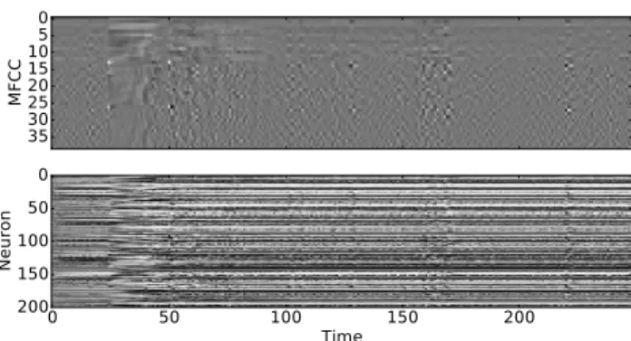
Natural inputs to a neural network tend to have a high degree of temporal autocorrelation, resulting in slowly-changing network states. This slow-slowly-changing activation feature is also seen within the computation of RNNs pro-cessing audio inputs, for example, speech (Fig.1). Delta networks, as introduced here, exploit the temporal stability of both the input stream and the associated neu-ral representation to reduce memory access and computa-tion without loss of accuracy. By caching neuron activa-tions, computations can be skipped where inputs change by a small amount from the previous update. Because each neuron that is not updated will save fetches of en-tire columns of several weight matrices, determining which
0 5 10 15 20 25 30 35 M F C C 0 50 100 150 200 Time 0 50 100 150 200 N e u ro n
Figure 1.Stability in RNN activations over time. The top figure shows the continually-changing MFCC features for a spoken digit from the TIDIGITS dataset (Leonard & Doddington,1993); the bottom figure shows the corresponding neural network output ac-tivations in response to these features. Note the slow evolution of the network states over timesteps.
neurons need to be updated offers significant speedups. The rest of the paper is organized as follows. Sec. 2 in-troduces the delta network concept in terms of the basic matrix-vector operations. Sec. 3 formulates it concretely for a GRU RNN. Sec.4proposes a method using a finite threshold for the deltas that suppresses the accumulation of the transient approximation error. Sec.5describes methods for optimally training a delta RNN. Sec.6shows network accuracy versus speedup for three examples. Finally, Sec.7
summarizes the results.
2. Delta Network Formulation
The purpose of a delta network is to transform a dense matrix-vector multiplication (for example, a weight ma-trix and a state vector) into a sparse mama-trix-vector multi-plication followed by a full addition. This transformation leads to savings on both operations (actual multiplications) and more importantly memory accesses (weight fetches). Fig.2illustrates the savings due to a sparse multiplicative vector. Zeros are shown with white, while non-zero matrix and vector values are shown in black. Note the multiplica-tive effect of sparsity in the weight matrix and sparsity in the delta vector. In this example, 20% occupancy of the weight matrix and 20% occupancy of the∆vector requires fetching and computing only 4% of the original operations. To illustrate the delta network methodology, consider a general matrix-vector multiplication of the form
r=W x (1)
that usesn2compute operations1,n2+nreads andnwrites
for a W matrix of size n×nand a vector xof size n.
1In this paper, a “compute” operation is either a multiply, an add, or a multiply-accumulate. The costs of these operations are
•
=
Weight Matrix
Delta
Vector Nonzero Operations
Figure 2.Illustration of saved matrix-vector computation using delta networks with sparse delta vectors and weight matrices.
Now consider multiple matrix-vector multiplications for a long input vector sequencextindexed byt= 1,2, . . . .The
resultrtcan be calculated recursively as:
rt=W∆ +rt−1, (2)
where∆ =xt−xt−1andrt−1is the result obtained from the previous calculation; if stored, the compute cost ofrt−1 is zero as it can be fetched from the previous timestep. Triv-ially,x0= 0andr0= 0. It is clear that
rt=W(xt−xt−1) +rt−1 (3)
=W(xt−xt−1) +W(xt−1−xt−2) +. . .+r0 (4)
=W xt (5)
Thus this formulation, which uses the difference between two subsequent timesteps and referred to as thedelta net-workformulation, can be seen to produce exactly the same result as the original matrix-vector multiplication.
2.1. Theoretical Cost Calculation
To illustrate the savings if∆from (2) is sparse, we begin by definingocto be theoccupancyof a vector , that is, the
percentage of nonzero elements in the vector.
Consider the compute cost forrt; it consists of the total
cost for calculating ∆ (n operations for a vector of size
n), adding in the stored previous resultrt−1(noperations),
and performing the sparse matrix multiplyW∆(oc·n2
op-erations for aW of sizen×nand a sparse∆vector of occupancy ratiooc). Similarly, the memory cost for
calcu-latingrtrequires fetchingoc·n2weights forW,2nvalues
for∆,nvalues forrt−1and writing out thenvalues forrt.
Overall, the compute cost for the standard formulation (Ccomp,dense) and the new delta formulation (Ccomp,sparse)
similar, particularly when compared to the cost of an off-chip memory operation. See (Horowitz,2014) for a simple compar-ison of energy costs of compute and memory operations.
will be:
Ccomp,dense=n2 (6)
Ccomp,sparse=oc·n2+ 2n (7)
while the memory access costs for both the standard (Cmem,dense) and delta networks (Cmem,sparse) can be seen
from inspection as:
Cmem,dense=n2+n (8)
Cmem,sparse=oc·n2+ 4n (9)
Thus, the arithmetic intensity (ratio of arithmetic to mem-ory access costs) asn→ ∞is 1 for both the standard and delta network methods. This means that every arithmetic operation requires a memory access, unfortunately placing computational accelerators at a disadvantage. However, if a sparse occupancyocof∆is assumed, then the decrease in
computes and memory accesses due to storing the previous state will result in a speedup of:
Cdense/Csparse≈n2/(oc·n2) = (1/oc) (10)
For example, ifoc= 10%, then the theoretical speedup will
be 10X. Note that this speedup is determined by the occu-pancy in each computed∆ =xt−xt−1, implying that this
sparsity is determined by the data stream. Specifically, the regularity with which values stay exactly the same between
xtandxt−1, or as demonstrated later, within a certain ab-solute value called the threshold, determines the speedup. In a neural network, xcan represent inputs, intermediate activation values, or outputs of the network. Ifxchanges slowly between subsequent timesteps then the input values
xtandxt−1will be highly redundant, leading to a low oc-cupancyocand a correspondingly increased speedup.
3. Delta Network GRUs
In GRUs, the matrix-vector multiplication operation that can be replaced with a delta network operation appears sev-eral times, shown in bold below. This GRU formulation is from (Chung et al.,2014):
rt=σr(Wxrxt+Whrht−1+br) (11)
ut=σu(Wxuxt+Whuht
−1+bu) (12)
ct=σc(Wxcxt+rt⊙(Whcht−1) +bc) (13)
ht= (1−ut)⊙ht−1+ut⊙ct (14)
Here r, u, c andhare reset and update gates, candidate activation, and activation vectors, respectively, typically a few hundred elements long. Theσfunctions are nonlinear logistic sigmoids that saturate at 0 and 1. The⊙signifies element-wise multiplication. Each term in bold can be
re-placed with the delta update defined in (2), forming:
∆x=xt−xt−1 (15) ∆h=ht−1−ht−2 (16) rt=σr(Wxr∆x+zxr+Whr∆h+zhr+br) (17) ut=σu(Wxu∆x+zxu+Whu∆h+zhu+bu) (18) ct=σc(Wxc∆x+zxc+bc rt⊙(Whc∆h+zhc)) (19) ht=(1−ut)⊙ht−1+ut⊙ct (20)
where the valueszxr,zxu,zxc, zhr,zhu,zhcare recursively
defined as the the stored result of the previous computation for the input or hidden state, i.e.:
zxr := zxr,t−1= Wxr(xt−1−xt−2) +zxr,t−2 (21)
The above operation can be applied for the other five values
zxu,zxc, zhr,zhu,zhc. The initial condition at timex0is
z0:= 0. Also, many of the additive terms in the equations
above, including the stored full-rank pre-activation states as well as the biases, can be merged into single values re-sulting into four stored memory values (Mr,Mu,Mxc, and
Mhr) for the three gates:
Mt−1:=zx,t−1+zh,t−1+b (22)
Finally, in accordance with the above definitions of the ini-tial state, the memories M are initialized at their corre-sponding biases, i.e.,Mr,0=br,Mu,0=bu,Mxc,0 =bc,
andMhr,0 = 0, resulting in the following full formulation
of the delta network GRU:
∆x=xt−xt−1 (23) ∆h=ht−1−ht−2 (24) Mr,t :=Wxr∆x+Whr∆h+Mr,t−1 (25) Mu,t:=Wxu∆x+Whu∆h+Mu,t−1 (26) Mxc,t:=Wxc∆x+Mxc,t−1 (27) Mhc,t :=Whc∆h+Mhc,t−1 (28) rt=σr(Mr,t) (29) ut=σu(Mu,t) (30) ct=σc(Mxc,t+rt⊙Mhc,t) (31) ht= (1−ut)⊙ht−1+ut⊙ct (32)
4. Delta Network Approximations
The formulations described in Secs.2and3are designed to give precisely the same answer as the original computation in the network. However, a more aggressive approach can be taken in the update, inspired by recent studies that have shown the possibility of greatly reducing weight precision in neural networks without giving up accuracy (Stromatias et al.,2015;Courbariaux et al.,2014). Instead of skipping
a vector-multiplication computation if a change in the ac-tivation∆ = 0, a vector-multiplication can be skipped if a value of∆is smaller than the threshold (i.e|∆i,t|<Θ,
whereΘis a chosen threshold value for a statei at time
t). That is, if a neuron’s hidden-state M activation has changed by less than Θsince it was last memorized, the neuron output will not be propagated, i.e., its∆value is set to zero for that update. Using this threshold, the network will not produce precisely the same result at each update, but will produce a result which is approximately correct. Moreover, the use of a threshold substantially increases ac-tivation sparsity.
Importantly, if a non-zero threshold is used with a naive delta change propagation, errors can accumulate over mul-tiple time steps through state drift. For example, if the in-put valuextincreases by nearlyΘon every time step, no
change will ever be triggered despite an accumulated sig-nificant change in activation, causing a large drift in error. Therefore, in our implementation, the memory records the last value causing an above-threshold change, not the dif-ference since the last time step.
More formally, we introduce the statesxˆi,t−1andˆhj,t−1. These states store thei−th input and the hidden state of the
j−th neurons, respectively, at their lastchange. The cur-rent inputxi,tand statehj,twill be compared against these
values to determine the∆. Then thexˆi,t−1andˆhj,t−1 val-ues will only be updated if the thresholdΘis crossed. The equations are shown below for xˆi,t−1 with similar equa-tions forˆhj,t−1:
ˆ
xi,t−1=
(
xi,t−1 if|xi,t−xˆi,t−1|>Θ
ˆ
xi,t−2 otherwise
(33)
∆xi,t=
(
xi,t−xˆi,t−1 if|xi,t−xˆi,t−1|>Θ
0 otherwise (34)
That is, when calculating the input delta vector∆xi,t
com-prised of each elementiat timet, the difference between two values are used: the current value of the inputxi,t, and
the value the last time the delta vector was nonzeroˆxi,t−1.
Furthermore, if the delta change is less thanΘ, then the delta change is set to zero, producing a small approxima-tion error that will be corrected when a sufficiently large change produces a nonzero update. The same formulation is used for the hidden state delta vector∆hj,t.
This input approximation does not guarantee that the output error is bounded by the same thresholdΘ. As supported by previous studies demonstrating that GRUs can be arbitrar-ily sensitive to input perturbations (Laurent & von Brecht,
2016), the ptimestep error can grow with the input er-ror. While thresholding should offer greater sparsity, the accumulation of these approximations could result in a di-verging output error, therefore motivating the experiments
in Sec.6.1that examine the effect of approximation on tra-jectory evolution.
5. Methods to Increase Accuracy & Speedup
This section presents training methods and optimization schemes for faster and more accurate delta networks.
5.1. Training Directly on Delta Networks
The most principled method of training to minimize accu-racy loss when running as a delta network would be to train directly on the delta network model. This should yield the best results as the network will receive errors that arise di-rectly from the truncations of the delta network computa-tion, and through training, learn to become robust to the types of errors that delta networks make.
More accurately, instead of training on the original GRU equations Eq. 11–14, the state is updated using the delta network model described in Eq.23–34. Importantly, this change should incur no accuracy loss between train accu-racy and test accuaccu-racy, though gradient descent may yet have more difficulty optimizing the model during training.
5.2. Rounding Network Activations
As the truncation of network activation due to the delta net-work is inherently non-differentiable, this training method should be compared against more widely used methods to verify its effectiveness. The delta network’s computation can be viewed as analogous to the reduced-precision round-ing trainround-ing methods; small changes are rounded to zero while larger changes are propagated. Since many previ-ous investigations have demonstrated methods to train net-works to be robust against small rounding errors by round-ing durround-ing trainround-ing (Courbariaux et al., 2014; Stromatias
et al.,2015), these methods can be leveraged here to train
a network that does not rely on small fluctuations in inputs. Low-precision computation and parameters can further re-duce power consumption and improve the efficiency of the network for dedicated hardware implementations.
As in other studies, a low-resolution activationθLin signed
fixed-point format Qm.f withminteger bits andf frac-tional bits can be produced from a high-resolution acti-vationθ by using a deterministic and gradient-preserving rounding: θL =round(2f·θ)·2−f with2f ·θclipped to
a bounding range[−2m+f−1,2m+f−1]to produce a quan-tized fixed-point activation. The output error cost forces the network to avoid quantization errors during training.
5.3. Adding Gaussian Noise to Network Activations
Random noise injection provides another useful compar-ison point. By injecting noise, the network will be
un-able to rely on small changes, and occasionally even larger changes will be incorrect (as may be the case of thresh-old rounding). This robustness can be provided by adding Gaussian noiseηto terms that will have a thresholded delta activation: rt=σr((xt+ηx)Wxr+ (ht−1+ηh)Whr+br) (35) ut=σu((xt+ηx)Wxu+ (ht−1+ηh)Whu+bu) (36) ct=σc((xt+ηx)Wxc+ rt⊙((ht−1+ηh)Whc) +bc) (37) ht= (1−ut)⊙ht−1+ut⊙ct (38)
whereη∼ N(µ, σ). That is,ηis a vector of samples drawn from the Gaussian distribution with meanµand varianceσ, andη ∈ {ηx, ηh}. Each element of these vectors is drawn
independently. Typically, the valueµis set to0so that the expectation is unbiased, e.g.,E[xt+ηx] =E[xt].
As a result, the Gaussian noise should prevent the network from being sensitive to minor fluctuations, and increase its robustness to truncation errors.
5.4. Considering Weight Sparsity
In all training methods, considering the additional speedup from weight sparsity, in addition to skipping activa-tion computaactiva-tion, should improve the theoretical speedup. Studies such as in (Ott et al.,2016) show that in trained low-precision networks, the weight matrices can be quite sparse. For example, in a ternary or 3-bit weight network the weight matrix sparsity can exceed 80% for small RNNs. Since every nonzero input vector element is multiplied by a column of the weight matrix, this computation can be skipped if the weight value is zero. That is, the zeros in the weight matrix act multiplicatively with the delta vector to produce even fewer necessary multiply-accumulates, as illustrated above in Fig.2. The compute cost of the matrix-vector product will beCcomp,sparse=om·oc·n2+ 2nand
the memory cost will beCmem,sparse =om·oc·n2+ 4n
for a weight matrix with occupancy om. By comparison
to Eq.10, the system can achieve a theoretical speedup of
1/(om·oc). That is, by compressing the weight matrix and
only fetching nonzero weight elements that combine with the nonzero state vector, a higher speedup can be obtained without degrading the accuracy.
5.5. Incurring Sparsity Cost on Changes in Activation
Finally, a computation-specific cost can be associated with the delta terms and added to the overall cost. In an input batch, theL1 norm for∆hcan be calculated as the mean
absolute delta changes, and this norm can be scaled by a weighting factorβ. ThisLsparsecost (Lsparse=β||∆h||1)
can then be additively incorporated into the standard loss function. Here the L1 norm is used to encourage sparse
values in∆h, so that fewer delta updates are required.
6. Results
This section presents results demonstrating the trade-off between compute savings and accuracy loss, using Delta Network RNNs trained on the TIDIGITS digit recognition benchmark. Furthermore, it also demonstrates that the re-sults found on small datasets also translate to the much larger Wall Street Journal speech recognition benchmark. The final example is for a CNN-RNN stack trained on end-to-end steering prediction using a recent driving dataset. The fixed-point Q3.4 (i.e. m = 3 andf = 4) format was used for network activation values in all speech ex-periments except the “Original” RNN line for TIDIGITS in Fig.4, which was trained in floating-point representa-tion. The driving dataset in Sec.6.4usedQ2.5activation. The networks were trained with Lasagne (Dieleman et al.,
2015) powered by Theano (Bergstra et al.,2010). Reported training time is for a single Nvidia GTX 980 Ti GPU.
6.1. TIDIGITS Dataset Trajectory Evolution
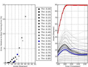
0 5 10 15 20 25 30 35 40 45 Angle [Degrees] 0 5 10 15 20 E rr o r, R e la ti v e t o B e st T ra in in g E rr o r [% ] Thr: 0.00 Thr: 0.05 Thr: 0.10 Thr: 0.15 Thr: 0.20 Thr: 0.25 Thr: 0.30 Thr: 0.35 Thr: 0.40 Thr: 0.45 Thr: 0.50 Thr: 0.55 Thr: 0.60 Thr: 0.65 Thr: 0.70 Thr: 0.75 Thr: 0.80 Thr: 0.85 160 180 200 220 240 Time [Timesteps] 0 10 20 30 40 50 60 70 80 90 A n g le [ D e g re e s]
Figure 3.Comparison of trajectories over time by increasingΘ
from 0 to 0.85 in steps of 0.05. At left, an increase of error an-gle between the final training state and the final thresholded state manifests as a decrease in accuracy, with the Gaussian-trained net as squares and DN-trained net as circles. At right, the mean angle between the unapproximated state and the thresholded state over time. In red, the angle over time of an untrained network that has the same weight statistics as a trained network; in solid lines, a network that was trained as a delta network; in dashed lines, a network that was only trained with Gaussian noise. Curves for
Θ = 0.55are highlighted in blue. Note that a DN-trained
net-work has lower angle error, especially at higher thresholds, and an untrained net always quickly converges to an orthogonal state.
The TIDIGITS dataset was used as an initial evaluation task to study the trajectory evolution of delta networks. Sin-gle digits (“oh” and zero through nine), totalling 2464
dig-its in the training set and 2486 digdig-its in the test set, were transformed in the standard way (Neil & Liu,2016) to pro-duce a 39-dimensional Mel-Frequency Cepstral Coefficient (MFCC) feature vector using a 25 ms window, 10 ms frame shift, and 20 filter bank channels. The labels for “oh” and “zero” were collapsed to a single label. Training time is approximately 8 minutes for a 150 epoch experiment. The network architecture consists of a layer of 200 GRU units connected to a layer of 200 fully-connected units and finally to a classification layer for the 10 digit classes. First, a network was trained with Gaussian noise injection (Sec.5.3) and subsequently tested using the delta network GRU formulation given in Sec.3. A second network was trained directly on the delta network GRU formulation in accordance with Sec. 5.1, with the same architecture and
Θ = 0.5. Finally, a third network was constructed from the DN-trained network by permuting its weights to produce an “untrained” network with identical weight statistics. To determine the robustness of the network to thresholded input, the trajectory evolution of these three networks were examined in comparison to their training conditions. Since the hidden states are bounded by (-1, 1) from the tanh non-linearity, each 200-dimensional hidden state vector is nor-malized to construct a unit vector. Then, the error angle be-tween the hidden state at training time and the hidden state with a threshold is measured. This error angle is correlated with the final accuracy, as seen in Fig.3left. The thresh-old is swept from 0 to 0.85, producing the results found in Fig.3right, in which each line represents the mean differ-ence angle over all states across time. The figure begins at the median start point of a digit presentation (t=158), as the digits are pre-padded with zeros to match lengths.
A Gaussian-trained network’s trajectory initially matches its training trajectory to produce a low error angle at low thresholds, which gradually increases as the threshold is raised. However, across a wide range ofΘ, a DN-trained net’s trajectory matches its training trajectory much more closely to produce a tighter-spaced arrangement and sub-stantially lower angle error at higher threshold. Finally, an untrained network is indeed very sensitive to input approx-imations and quickly reaches an orthogonal representation, thus emphasizing the role of training to provide robustness.
6.2. TIDIGITS Dataset Speedup and Accuracy
The results of applying the methods introduced in Sec. 5
can be found in Fig.4. There are two quantities measured: the change in the number of memory fetches, and the accu-racy as a function of the thresholdΘ. Fig.5shows the same results, but removes the threshold axis to directly compare the accuracy-speedup tradeoff among the different training methods. First, a standard GRU RNN achieving 96.59% accuracy on TIDIGITS was trained without data
augmen-0.0 0.1 0.2 0.3 0.4 0.5 0.6 0.7 0.8 0.9 Threshold at Test 90 91 92 93 94 95 96 97 98 99 A cc u ra cy [ % , S o lid ] 1 1a 1ab 2a2, 2ab 1: Original
1a: + Rounding during Train 1ab: + Noise
2: Train on DN
2a: + Account for Sparse Weights 2ab: + L1 Cost 0 2 4 6 8 10 12 14 S p e e d u p F a ct o r [D a sh e d ]
Figure 4.Test accuracy results from standard GRUs run as delta networks after training (curves1,1a, and1ab) and those trained as delta networks (curves 2, 2a, and 2ab) under different con-straints on the TIDIGITS dataset. The delta networks are trained
forΘ = 0.5, and the average of five runs is shown. Note that
the methods are combined, hence the naming scheme. Addition-ally, the accuracy curve for2is hidden by the curve2a, since both achieve the same accuracy and only differ in speedup metric.
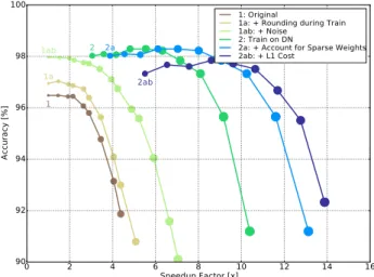
0 2 4 6 8 10 12 14 16 Speedup Factor [x] 90 92 94 96 98 100 A cc u ra cy [ % ] 1 1a 1ab 2 2a 2ab 1: Original
1a: + Rounding during Train 1ab: + Noise
2: Train on DN
2a: + Account for Sparse Weights 2ab: + L1 Cost
Figure 5.Accuracy-speedup tradeoff by adjustingΘfor
TIDIG-ITS. By increasing Θ (indicated by sample point size), larger speedups can be obtained at greater losses of accuracy. For net-works trained as delta netnet-works, the training threshold is the first (leftmost) point in the line point sequence.
tation and regularization. This network has the architecture described in Sec.6.1. It was then subsequently tested using the delta network GRU formulation given in Sec.3. The standard RNN run as a delta network (“Original”) achieves 95% accuracy (a drop from zero delta threshold accuracy of 96%) with a speedup factor of about 2.2X. That is, only approximately 45% of the computes or fetches are needed in achieving this accuracy. By adding the
round-ing constraint durround-ing trainround-ing (“+ Roundround-ing durround-ing Train-ing”), the accuracy is nearly 97% with an increase to a 3X speedup. By incorporating Gaussian noise (“+ Noise”), 97% accuracy can be maintained with a 5X speedup. Es-sentially, these methods added generalization robustness to the original GRU, while preventing small changes from in-fluencing the network output. These techniques allow a higher threshold to be used while maintaining the same ac-curacy, therefore resulting in a decrease of memory fetches and a corresponding speedup.
The best model for training is the delta network itself (“Train on DN”). This network achieved 97.5% accuracy with a 8X speedup. Accounting for the pre-existing spar-sity in the weight matrix (“+ Account for Sparse Weights”), the speedup increases to 10.5X, without affecting the accu-racy (since it is the same network). Finally, incorporating an L1 cost on network changes in addition to training on the delta network model (“+ L1 cost”) achieves 97% accu-racy while boosting speedup to 11.9X. Adding in the final sparseness cost on network changes decreases the accuracy slightly since the loss minimization must find a tradeoff be-tween both error and delta activation instead of considering error alone. However, using the L1 loss can offer a sig-nificant additional speedup while retaining an accuracy in-crease over the original GRU network.
Finally, Fig. 5 also demonstrates the primary advantage given by each algorithm; an increase in generalization ro-bustness manifests as an overall upward shift in accuracy, while an increase in sparsity manifests as a rightward shift in speedup. As proposed, methods 1a and 1b increase gen-eralization robustness while only modestly influencing the sparsity. Method 2 greatly increases both, while method 2a only increases sparsity, and finally method 2ab slightly decreases accuracy but offers the highest speedup.
6.3. Wall Street Journal Dataset
The delta network methodology was applied to an RNN trained on the larger WSJ dataset to determine whether it could produce the same gains as seen with the TIDIGITS dataset. This dataset comprised 81 hours of transcribed speech, as described in (Braun et al.,2016). Similar to that study, the first 4 layers of the network consisted of bidirec-tional GRU units with 320 units in each direction. Training time for each experiment was about 120h.
Fig. 6 presents results on the achieved word error rate (WER) and speedup on this dataset for two cases: First, running an existing speech transcription RNN as a delta network (results shown as solid curves labeled “RNN used as a DN”), and second, a network trained as a delta network with results shown as the dashed curves “Trained Delta Network”. The speedup here accounts for weight matrix sparsity as described in Sec.5.4.
0.0 0.1 0.2 0.3 0.4 0.5 Threshold 0 2 4 6 8 10 12 R e d u ct io n i n O p s [M u lt ip le s] 1.3x 3.1x 4.2x 4.7x 5.7x 6.2x 7.3x 8.5x 9.1x 10.3x 0 10 20 30 40 50 W o rd E rr o r R a te 10.2% 10.2% 10.2% 10.4% 10.8% 11.0% 12.1% 13.2% 14.2% 16.3% Trained Delta Network
GRU Network used as a DN
Figure 6.Accuracy and speedup tradeoffs on the WSJ dataset. The solid lines show results from an existing deep RNN run as a delta network. The dashed lines show results from a network trained as a delta network withΘ = 0.2. The horizontal lines indicate the non-delta network accuracy level; similarly, the solid and dashed horizontal lines indicate the accuracy of the normal network and the DN network prior to rounding, respectively.
Surprisingly, the existing highly trained network already shows significant speedup without loss of accuracy as the threshold, Θ, is increased: At Θ = 0.2, the speedup is about 5.5X with a WER of 10.8% compared with the WER of 10.2% at Θ = 0. However, training the RNN to run as a delta network yields a network that achieves a slightly higher 5.7X speedup with the same WER. Thus, even the conventionally-trained RNN run as a delta network can provide greater than 5X speedup with only a 1.05X in-crease in the WER.
6.4. Comma.ai Driving DataSet
Driving scenarios are rapidly emerging as another area of RNN focused research. Here, the delta network model was applied to determine the gains of exploiting the redun-dancy of real-time video input. The open driving dataset from comma.ai (Santana & Hotz,2016) with 7.25 hours of driving data was used, with video data recorded at 20 FPS from a camera mounted on the windshield. The network is trained to predict the steering angle from the visual scene similar to (Hempel,2016;Bojarski et al.,2016). We fol-lowed the approach in (Hempel,2016) by using an RNN on top of the CNN feature detector. The CNN feature detector has three convolution layers without pooling layers and a fully-connected layer with 512 units. During training, the CNN feature detector was pre-trained with an analog out-put unit to learn the recorded steering angle from randomly selected single frame images. Afterwards, the delta net-work RNN was added, and trained by feeding sequences of the visual features from the CNN feature detector to learn
Figure 7.Reduction of RNN compute cost in the steering angle prediction task. Top figure shows the required # of ops per frame for the delta network GRU layer (trained withΘ = 0.1) in com-parison with the conventional GRU case. Bottom figure compares the prediction errors of CNN predictor and CNN+RNN predictor. The RNN slightly improves the steering angle prediction.
sequences of the steering angle. Since the Q2.5 format was used for the GRU layer activations, the GRU input vectors were scaled to match the CNN output and the target output was scaled to match the RNN output.
However, this raw dataset results in a few practical diffi-culties and requires data preprocessing. By excluding the frames recorded during periods of low speed driving, we remove the segments where the steering angle is not corre-lated to the direction of the car movement. Training time of the CNN feature detector was about 8h for 10k updates with the batch size of 200. Training of the RNN part took about 3h for 5k updates with the batch size of 32 samples consisting of 48 frames/sample.
A very large speedup exceeding 100X in the delta network GRU can be seen in Fig.7, computed for the steering angle prediction task on 2000 consecutive frames (100s) from the validation set. While the number of operations per frame remains constant for the conventional GRU layer, those for the delta network GRU layer varies dynamically depending on the change of visual features.
In this steering network, the computational cost of the CNN (about 37 MOp/frame) dominates the RNN cost (about 1.58 MOp/frame), therefore the overall system-level com-putational savings is only about 4.2%. However, future ap-plications will likely have efficient dedicated vision hard-ware or require a greater role for RNNs in processing nu-merous and complex data streams, which result in RNN models that consume a greater percentage of the overall en-ergy/compute cost. Even now, the steering angle prediction network already benefits from a delta network approach.
7. Discussion and Conclusion
Although the delta network methodology can be applied to other network architectures, as was shown in similar
con-CNN only Speedup 100 200 300 400 0.0 0.1 42x 67x 137x 177x 253x 324x 354x 405x 0.2 0.3 0.5 Delta Threshold 0.4 27
RMS Prediction Error (deg)
28 29 30 31 32 33
Figure 8.Tradeoffs between prediction error and speedup of the GRU layer on the steering angle prediction. The result was ob-tained from 1000 samples with 48 consecutive frames sampled from the validation set. Speedup here does not include weight ma-trix sparsity. The network was trained withΘ = 0.1. A speedup of approximately 100X can be obtained without increasing the prediction error, usingΘbetween 0.1 and 0.25.
current work for CNNs (O’Connor & Welling,2016), in practice a larger benefit is seen in RNNs because all the intermediate activation values for the delta networks are al-ready stored between subsequent inputs. For example, the widely-used VGG19 CNN has 16M neuron states (
Chat-field et al.,2014). Employing the delta network approach
for CNNs requires doubled memory access and significant additional memory space to store the entirety of the net-work state. Because the cost of external memory access is hundreds of times larger than that of arithmetic operations, delta network CNNs seem impractical without novel mem-ory technologies to address this issue.
In contrast, RNNs have a much larger number of weight parameters than activations. The sparsity of the delta ac-tivations can therefore enable large savings in power con-sumption by reducing the number of memory accesses re-quired to fetch weight parameters. CNNs, however, do not have this advantage since the weight parameters are few and shared by many units. Finally, the delta network ap-proach is extremely flexible as pre-existing networks can be used without retraining, or trained specifically for in-creased optimization.
Recurrent neural networks can be highly optimized due to the redundancy of their activations over time. When the use of this temporal redundancy is combined with robust training algorithms, this work demonstrates that speedups of 6X to 9X can be obtained with negligible accuracy loss in speech RNNs, and speedups of over 100X are possible in steering angle prediction RNNs, suggesting significant speedups are achievable on practical, real-world problems.
Acknowledgements
We thank S. Braun for helping with the WSJ speech tran-scription pipeline. This work was funded by Samsung In-stitute of Advanced Technology, the University of Zurich and ETH Zurich.
References
Amodei, Dario, Anubhai, Rishita, Battenberg, Eric, Case, Carl, Casper, Jared, Catanzaro, Bryan, Chen, Jingdong, Chrzanowski, Mike, Coates, Adam, Diamos, Greg, et al. Deep speech 2: End-to-end speech recognition in english and mandarin. arXiv preprint arXiv:1512.02595, 2015. Bergstra, James, Breuleux, Olivier, Bastien, Fr´ed´eric,
Lamblin, Pascal, Pascanu, Razvan, Desjardins, Guil-laume, Turian, Joseph, Warde-Farley, David, and Ben-gio, Yoshua. Theano: a CPU and GPU math expres-sion compiler. InProceedings of the Python for scientific computing conference (SciPy), volume 4, pp. 3, 2010. Bojarski, Mariusz, Testa, Davide Del, Dworakowski,
Daniel, Firner, Bernhard, Flepp, Beat, Goyal, Prasoon, Jackel, Lawrence D., Monfort, Mathew, Muller, Urs, Zhang, Jiakai, Zhang, Xin, Zhao, Jake, and Ziebam, Karol. End to end learning for self-driving cars. arXiv preprint arXiv:1604.07316, 2016.
Braun, Stefan, Neil, Daniel, and Liu, Shih-Chii. A cur-riculum learning method for improved noise robust-ness in automatic speech recognition. arXiv preprint arXiv:1606.06864, 2016.
Chatfield, Ken, Simonyan, Karen, Vedaldi, Andrea, and Zisserman, Andrew. Return of the devil in the details: Delving deep into convolutional nets. arXiv preprint arXiv:1405.3531, 2014.
Cho, Kyunghyun, van Merrienboer, Bart, Gulcehre, Caglar, Bougares, Fethi, Schwenk, Holger, and Bengio, Yoshua. Learning phrase representations using RNN encoder-decoder for statistical machine translation. arXiv preprint arXiv:1406.1078, 2014.
Chung, Junyoung, Gulcehre, Caglar, Cho, KyungHyun, and Bengio, Yoshua. Empirical evaluation of gated re-current neural networks on sequence modeling. arXiv preprint arXiv:1412.3555, 2014.
Courbariaux, Matthieu and Bengio, Yoshua. Bina-rynet: Training deep neural networks with weights and activations constrained to+ 1 or-1. arXiv preprint arXiv:1602.02830, 2016.
Courbariaux, Matthieu, Bengio, Yoshua, and David, Jean-Pierre. Low precision arithmetic for deep learning.arXiv preprint arXiv:1412.7024, 2014.
Courbariaux, Matthieu, Bengio, Yoshua, and David, Jean-Pierre. Binaryconnect: Training deep neural networks with binary weights during propagations. InAdvances in Neural Information Processing Systems, pp. 3123–3131, 2015.
Dieleman, Sander et al. Lasagne: First release., Au-gust 2015. URLhttp://dx.doi.org/10.5281/ zenodo.27878.
Esser, Steven K, Merolla, Paul A, Arthur, John V, Cassidy, Andrew S, Appuswamy, Rathinakumar, Andreopoulos, Alexander, Berg, David J, McKinstry, Jeffrey L, Melano, Timothy, Barch, Davis R, et al. Convolutional net-works for fast, energy-efficient neuromorphic comput-ing.arXiv preprint arXiv:1603.08270, 2016.
Graves, Alan, Mohamed, Abdel-rahman, and Hinton, Ge-offrey. Speech recognition with deep recurrent neural networks. InAcoustics, Speech and Signal Processing (ICASSP), 2013 IEEE International Conference on, pp. 6645–6649. IEEE, 2013.
Han, Song, Mao, Huizi, and Dally, William J. Deep com-pression: Compressing deep neural network with prun-ing, trained quantization and huffman coding. CoRR, abs/1510.00149, 2, 2015.
Han, Song, Kang, Junlong, Mao, Huizi, Hu, Yiming, Li, Xin, Li, Yubin, Xie, Dongliang, Luo, Hong, Yao, Song, Wang, Yu, et al. Ese: Efficient speech recognition engine with compressed lstm on fpga. In FPGA 2017; NIPS
2016 EMDNN workshop, 2016.
Hempel, Martin. Deep learning for piloted driving. In NVIDIA GPU Tech Conference, 2016.
Hochreiter, Sepp and Schmidhuber, J¨urgen. Long short-term memory. Neural computation, 9(8):1735–1780, 1997.
Horowitz, M. 1.1 Computing’s energy problem (and what we can do about it). In2014 IEEE International Solid-State Circuits Conference Digest of Technical Papers (ISSCC), pp. 10–14, February 2014. doi: 10.1109/ ISSCC.2014.6757323.
Huang, Gao, Sun, Yu, Liu, Zhuang, Sedra, Daniel, and Weinberger, Kilian. Deep networks with stochastic depth.arXiv preprint arXiv:1603.09382, 2016.
Iandola, Forrest N, Moskewicz, Matthew W, Ashraf, Khalid, Han, Song, Dally, William J, and Keutzer, Kurt. Squeezenet: Alexnet-level accuracy with 50x fewer parameters and¡ 1mb model size. arXiv preprint arXiv:1602.07360, 2016.
Laurent, Thomas and von Brecht, James. A recur-rent neural network without chaos. arXiv preprint arXiv:1612.06212, 2016.
Leonard, R Gary and Doddington, George. Tidigits speech corpus.Texas Instruments, Inc, 1993.
Mikolov, Tomas, Karafi´at, Martin, Burget, Lukas, Cer-nock`y, Jan, and Khudanpur, Sanjeev. Recurrent neu-ral network based language model. InInterspeech, vol-ume 2, pp. 3, 2010.
Neil, Daniel and Liu, Shih-Chii. Effective sensor fusion with event-based sensors and deep network architec-tures. InIEEE Int. Symposium on Circuits and Systems (ISCAS), 2016.
O’Connor, Peter and Welling, Max. Sigma delta quantized networks. arXiv preprint arXiv:1611.02024, 2016. Ott, Joachim, Lin, Zhouhan, Zhang, Ying, Liu,
Shih-Chii, and Bengio, Yoshua. Recurrent neural net-works with limited numerical precision. arXiv preprint arXiv:1608.06902, 2016.
Rastegari, Mohammad, Ordonez, Vicente, Redmon, Joseph, and Farhadi, Ali. Xnor-net: Imagenet classifica-tion using binary convoluclassifica-tional neural networks. arXiv preprint arXiv:1603.05279, 2016.
Santana, Eder and Hotz, George. Learning a driving simu-lator. arXiv preprint arXiv:1608.01230, 2016.
Stromatias, Evangelos, Neil, Daniel, Pfeiffer, Michael, Galluppi, Francesco, Furber, Steve B, and Liu, Shih-Chii. Robustness of spiking Deep Belief Networks to noise and reduced bit precision of neuro-inspired hard-ware platforms.Frontiers in Neuroscience, 9, 2015. Szegedy, Christian, Liu, Wei, Jia, Yangqing, Sermanet,
Pierre, Reed, Scott, Anguelov, Dragomir, Erhan, Du-mitru, Vanhoucke, Vincent, and Rabinovich, Andrew. Going deeper with convolutions. In Proceedings of the IEEE Conference on Computer Vision and Pattern Recognition, pp. 1–9, 2015.
Xu, Kelvin, Ba, Jimmy, Kiros, Ryan, Courville, Aaron, Salakhutdinov, Ruslan, Zemel, Richard, and Bengio, Yoshua. Show, attend and tell: Neural image cap-tion generacap-tion with visual attencap-tion. arXiv preprint arXiv:1502.03044, 2015.
Yao, Li, Torabi, Atousa, Cho, Kyunghyun, Ballas, Nico-las, Pal, Christopher, Larochelle, Hugo, and Courville, Aaron. Describing videos by exploiting temporal struc-ture. InProceedings of the IEEE International Confer-ence on Computer Vision, pp. 4507–4515, 2015.