Feature Interaction Detection by Pairwise
Analysis of LTL Properties - a case study
Muffy Calder and Alice Miller
Department of Computing Science University of Glasgow
Glasgow, Scotland. muffy,[email protected]
AbstractA Promela specification and a set of temporal properties are developed for a basic call service with a number of features. The properties are expressed in the logic LTL.
Interactions between features are detected by pairwise analysis of features and properties. The analysis quickly results in both state-space and property case explosion. To overcome this state-spaces are minimised, model checking re-sults generalised through symmetry and bisimulation, and analysis performed automatically using scripts. The result is a more extensive feature interaction analysis than others in the field.
Keywords communicating processes, distributed systems, model checking, feature interaction, communications services.
1
Introduction
In software development afeatureis a component of additional functionality – ad-ditional to the main body of code. Typically, features are added incrementally, at various stages in the life-cycle, by different developers. A consequence of adding features in this way is feature interaction, where the behaviour of one feature modifies the behaviour of another, often leading to unpredicted and/or unde-sirable results. The problem is a long standing one within the communications services domain [37, 3] and exhibits in many other component-based domains. Detection of interactions is crucial to any solution (whether system redesign or a run-time solution), but in complex systems, especially when there is a prolif-eration of features, detection by manual inspection is not feasible. Automated techniques are therefore essential. In this paper we use a combination of model checking, symmetry and scripting for detecting interactions.
After introducing the preliminaries in Section 2, the paper has two parts. First, in Sections 3 to 6, we develop a specification in Promela [26, 30] for a basic call service. Promela is an appropriate language because the service is inherently concurrent, with asynchronous communication. We develop a set of temporal properties in order to validate the specification. We discuss how to express the properties in the linear temporal logic LTL, and how to verify them
using the model checker SPIN1 [27], paying particular attention to state-space reduction.
Second, in Sections 7 to 10, we develop a feature set and perform pairwise interaction analysis. The analysis is completely automated, making extensive use of Perl scripts to generate the model checking runs. In section 11 we introduce a method based on abstraction and induction whereby we show how some of our results can be generalised for systems consisting of any number of users, in which at most two users have features.
We compare our results with others in the field in Section 12 and present our conclusions in Section 13. Some preliminary results have been presented earlier [4]; our analysis here is more extensive because we consider 9 features whereas previously 6, less complex, features were considered. We also employ symmetry, generalisation and include greater implementation detail.
2
Background
2.1 Communications Services and Feature Interactions
Our concern is the control of calls between two parties, the actual data exchanged (e.g. audio or digital) is not of interest. Control is provided by aservice, in classi-cal telecommunications, this is provided by a (stored program control) exchange. The service responds to events such as handset on or off hook, as well as sending control signals to devices and lines such as ringing tone or line engaged. Afeature
is additional functionality, for example, acall forwarding capability, orring back when free; a user is said tosubscribeto a feature. An interaction is a behavioural modification between two or more features and/or a service.
As an example, consider a user who subscribes to call waiting (CW) and
call forward when busy(CFB) and is engaged in a call. What will happen when there is a further incoming call? (Full details of all features mentioned here are given in section 7.) If the call is forwarded, then the CW feature is clearly compromised. If, on the other hand, call waiting is activated, then the CFB feature is compromised. Clearly both features cannot proceed as they would in isolation. This interaction is relatively simple (e.g. it can be seen as inconsistent requirements) because both features are subscribed to by a single user. We refer to this situation as a single user (SU) interaction. More subtle interactions can occur when more than one user/subscriber are involved, these are referred to as multiple user, (MU) interactions. For example, consider the scenario where user A subscribes tooriginating call screening (OCS), with user C on the screening list, and user B subscribes to CFB to user C. If A calls B, and the call is forwarded to C (as required by B’s feature CFB), then A’s feature OCS is compromised. On the other hand, if the call is not forwarded, then B’s CFB feature is compromised. These kind of interactions (i.e. MU) can be very difficult to detect (and resolve), particularly since different features may be activated at different stages of a the call cycle.
Interactions may be characterised informally as type I or type II [24]. Interac-tions which arise from inconsistent specificaInterac-tions, e.g. inconsistent state changes or inconsistent events, are called type I. These interactions are usually the result of a “shared trigger”, for example, in the case of CW and CFB above, both features are triggered by an incoming call. Type II interactions do not involve a shared trigger but still result in inconsistent user intentions, as demonstrated by the interaction above between OCS and CFB. Type II interactions can only be detected with reference to user intentions, i.e. properties of features; they are the primary concern of this paper.
2.2 Call Control and Feature Reference Models
There are numerous call models and feature sets in the literature. Since our motivation is detecting type II interactions, we take a user perspective, following theIN(Intelligent Networks) model, distributed functional plane [34]. Our basic call model is adapted from this standard, as follows.
Basic Call We implement the IN BCSM (basic call state model) with minor amendments:
– We unify the two null states (originating and terminating) O N ull and
T N ullinto the stateO/T N ull.
– Since routing is not our concern (we assume a single network), we merge the states Auth Orig Att, Collect Inf o, Analyse Inf o, Select Route and
Auth Call Setupinto the single stateAuth Orig Att.
– We separate theO Exceptionstate into two states, depending on the trigger eventsnoanswerandbusy, thus the states areO N o AnswerandO Busy.
– We make call tear down asymmetric. This reflects the behaviour of the UK PSTN and results in behaviour which is potentially more interesting than a symmetric tear down.
The BCSM is only a state model, there are no intentions, or explicit proper-ties given in this standard. We therefore introduce a set of properproper-ties based on practical experience and properties presented in the feature interaction literature [37, 3].
Features It is more difficult to select a standard feature set. Although the
IN Capability Set 1 (CS-1) [34] enumerates a number of features, behaviour is not defined. Most detailed descriptions of commercial features are proprietary. We have therefore chosen a feature set which is based on published literature, namely the feature set used in an SMV-based study [48]. Details of the feature set are given in section 7; comparison of this work with the SMV study is given in section 12.
2.3 Promela and SPIN
Promela, Process meta language [26, 27, 30], is a high-level, state-based, lan-guage for modelling communicating, concurrent processes. It is an imperative, C-like language with additional constructs for non-determinism, asynchronous and rendezvous (synchronizing) communication, dynamic process creation, and mobile connections, i.e. communication channels can be passed along other com-munication channels. The language is very expressive, and has intuitive Kripke structure semantics.
Definition 1. Let AP be a set of atomic propositions. A Kripke structure over AP is a tupleM= (S, S0, R, L)where S is a finite set of states,S0 ⊆S is the set of initial states, R ⊆S×S is a transition relation and L :S → 2AP is a function that labels each state with the set of atomic propositions true in that state.
From here on we assume that|S0|= 1, i.e. there is a single initial state,s0say. SPINis a bespoke model checker for Promela and provides several reasoning mechanisms: assertion checking, acceptance/progress states and cycle detection and satisfaction of temporal properties. These properties are expressed in tem-poral logic [41, 17, 16]. The logic used is linear temporal logic LTL [49]. When performing verification, we use XSPIN, the graphical interface for SPIN.
We note that in the context of model checking the terms “model”, “speci-fication” and “system” are easily confused. Here we try to adopt the following convention: a model is Kripke structure, a specification is a Promela description (from which a Kripke structure is derived), and a system is a commonly under-stood physical implementation or abstraction thereof. We note that there are further uses of these terms, e.g. the basic call model.
Other popular model checkers include SMV [45], Murphi [13], FDR [50] and the Java PathFinder model checker JPF [55]. We choose to work with Promela and SPINprimarily because of the rich, expressive power of Promela, in partic-ular, asynchronous communication. SPIN has been widely used to model check protocols associated with software-controlled systems, for example, in commu-nications systems [5, 4, 32] and in railway interlocking systems [8].
2.4 Reasoning in SPIN
In order to perform verification on a specification, SPIN translates each process template into a finite automaton and then computes an asynchronous interleav-ing product of these automata to obtain the global behaviour of the concurrent system. This interleaving product is referred to as thestate-space.
As well as enabling a search of the state-space to check for deadlock, assertion violations etc., SPIN allows the checking of the satisfaction of an LTL formula over all execution paths. The mechanism for doing this is vianever claims– pro-cesses which describe undesirable behaviour, and B¨uchi automata – automata that accept a system execution if and only if that execution forces it to pass
through one or more of its accepting states infinitely often [27, 22, 44]. Checking satisfaction of a formula involves the depth-first search of the synchronous prod-uct of the automaton corresponding to the concurrent system (model) and the B¨uchi automaton corresponding to the never-claim.
Note that B¨uchi automata are more expressive than LT L itself (there are behaviours that can be expressed directly as B¨uchi automata that can not be expressed as LTL formulae). However, we find LTL to be quite adequate to describe the behaviour of our system, and prefer to allow SPIN’s excellent LTL converter to create the B¨uchi automata for us. Other formalisms exist to express behaviour (e.g. timelines [53], or Message sequence charts [43]). We do not use either of these methods here. We do use the MSC illustration of counterexamples provided by SPINhowever.
If the original LTL formulafdoes not hold, the depth-first search will “catch” at least one execution sequence for which¬fis true. Iff has the form []p, (that is
f is asafetyproperty), this sequence will contain anacceptance stateat which¬p
is true. Alternatively, iff has the formp, (that isf is alivenessproperty), the sequence will contain a cycle which can be repeated infinitely often, throughout which ¬pis true. In this case the never-claim is said to contain an acceptance cycle. In either case the never claim is said to bematched.
When using XSPIN’s LTL converter it is possible to check whether a given property holds forAll Executionsor forNo Executions. A universal quantifier is implicit in the beginning of all LTL formulas and so, to check an LTL property it is natural, therefore, to choose theAll Executionsoption. However, we sometimes wish to check that a given property (psay) holds alongsome execution path. This is not possible using LTL alone. However, SPINcan be used to show that “pholds forNo Executions” isnottrue (via a never-claim violation), which is equivalent. Therefore, when listing our properties (section 5.2), we use the shorthandEp
(meaningfor some pathp) to mean “(pfor No Executions) is not true”.
2.5 Parameters and Further Options used in SPINVerification When performing verification with SPIN three numeric parameters must be set. These arePhysical Memory Available,Estimated State-Space SizeandMaximum Search Depth. The meaning of the first of these is clear, and the second controls the size of the state-storage hash table. TheMaximum Search Depthparameter determines the size of the search-stack, where the states in the current search are stored. If comparisons are to be made with other model checkers, then the value of the Maximum Search Depth should be taken into account because its value determines the size of the stack provided for state storage, and so affects the total memory used. For this reason, in our verification results (see section 6.3 for example) we give only the memory required for state storage, and not the total memory required.
Partial order reduction (POR) [47, 46] is based on the observation that ex-ecution sequences (or “traces”) can be divided into equivalence classes whose members are indistinguishable with respect to a property that is to be checked. We apply POR in most cases.
Compression (COM) [28] is a method by which each individual state is en-coded in a more efficient way. We apply compression in all cases.
Weak Fairness (WF) is a constraint which ensures that the only paths con-sidered are those in which any process that has has an enabled transition will eventually do so. The use of WF is expensive, as it involves several copies of the state space being maintained, and so we avoid its use whenever possible (see section 9).
This concludes the background material, we are now ready to begin the first phase of the approach: a description of the basic call service.
3
Basic Call Service
In the next section we give an overview of the Promela specification. The spec-ification is quite detailed and so by way of introduction, in this section we give a more abstract behaviour description.
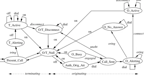
Figure 1 gives a diagrammatic representation of the automaton for the basic call service. States to the left of the O/T Null state represent terminating be-haviour, states to the right representoriginatingbehaviour. Events observable by service subscribers label transitions:user-initiatedevents at the terminal device, such as (handset) on and (handset) off, are given in plain font,network-initiated
events such asO/T Disconnectandengagedare given in italics. Note that there are two “ring” events,oringandtring, for originating and terminating ring tone, respectively. This reflects the fact that the ringing tone is indeed generated at each terminal device. Not all transitions are labelled. For example, there is an unlabelled transition from the (originating) stateCall SenttoO Alerting, simply because there is noobservableevent associated with this transition.
O/T_Null Auth_Orig_Att O_Busy O_No_Answer on terminating originating on unobt on off dial on off on T_Active tring tring Present_Call disconnect dial off on engaged on dial dial O/T_Disconnect disconnect dial Call_Sent O_Alerting dial oring O_Active connect oring T_Alerting
The automata must communicate with each other; the behaviour of one call process, as originating party, influences the behaviour of another call process, as terminating party. Since our motivation here is explanation rather than rigorous specification (that is the role of the Promela specification), we do not extend the automata to include a communication mechanism, rather we describe the communication informally.
A communication channel is associated with each call process. Each channel has capacity for at most one message: a pair consisting of a channel name (that associated with itself or the other party in the call) and a status bit (the status of the connection). When it is not confusing, we refer to the communication channel associated with call process A as channel A. When a communication channel is empty, then its associated call process is not connected to, or attempting to connect to, any other call process. When a communication channel is not empty, then the associated call process is engaged in a call, but not necessarily connected to another user. The interpretation of messages is described more comprehensively in Figure 2.
The communication channels are used to coordinate call set up and clear down. The basic protocol for call set up from A to B is as follows, assuming neither are engaged in a call. When A goes off hook, the message (A,0) is placed on channel A. After dialing B, the message (A,0) is sent to channel B. When B receives this message, the message (B,1) is sent to channel A and the status bit in the message on channel B is changed to 1; the connection is then established. To clear down, A can close down one side of the connection by going on hook: the message is removed from its communication channel and the status bit of the message in channel B is changed to 0. Then, since both A and B have status bit 0, neither process is in a connected state, and A is free to close down the connection. On the other hand, channel B cannot close down the connection (reflecting the real-life situation). So, if B goes on hook, while A and B are connected, then the connection status remains unchanged for both A and B.
Contents of ChannelA Interpretation
A is free
A is engaged, but not connected
B is attempting connection
If channel B contains (A,1) then A and empty
(B,1) (A,0)
A is engaged, but not connected (B,0)
B are connected B is terminating party
4
Basic Call Service in Promela
Each call process (see figure 1) is described in Promela as an instantiation of the (parameterised) proctype User declared thus:
proctype User (byte selfid;chan self)
Promela is a state-based formalism, therefore, we represent events by (their effect on) event variables (e.g.event[i] ornetwork event[i]) and call states (e.g.
Call Sent, Auth Orig Att, etc.) by labels. Since each transition is implemented by several (possibly compound) statements, we group these together as anatomic
statement, concluding with the appropriategoto.
An example of the Promela code associated with theO/T Null,Auth Orig Att,
Call Sent and O Active states and their outgoing transitions is given below. The global/local variables and parameters include the self-explanatory selfid
andpartnerid, the communication channel associated with the specific process
self, thepartner array, recording the channel name of the current partner of each process, the arraysconnect.to, recording the presence of a connection be-tween two users, the local variabledevrecording the current status of the device (on or off), the dialed array recording the most recent number dialed (since leaving theO/T Nullstate) for each process, and theeventandnetwork event
events recording the most recent user-initiated and network-initiated events of each process, respectively. In additionmesschanandmessbitare local variables used for reading messages. The channelnullallows a default value for any of the
partnervariables when the corresponding call process is not engaged in a call. This value is not strictly necessary for modelling purposes, but can be valuable for reasoning. Note that we use 6 as a default value (for thepartneridvariable for example) of variables which can take the value of any process id.
Any variable about which we may intend to reason should not be updated more than once within any atomic statement (so that each change to the vari-ables is visible to the never-claim), other varivari-ables may of course be updated as required. For this reason we have introduced a new state, O Close so that we can monitor when a connection has been made successfully. Thus the connec-tion is established within theO Activestate, via the setting of the array element
connect[self id].to[partnerid] to 1, and the remaining behaviour usually associ-ated with the O Active state is contained within O Close. (The full code for theO Closestate may be found in Appendix 1.) Finally, we note that there are numerous in-line assertions within the code, particularly at points when entering a new (call) state, and when reading and writing to communication channels.
O/T_Null: atomic{
assert(dev == on);
assert(partner[selfid]==null); /* either attempt a call, or receive one */
if
:: empty(self)->event[selfid]=off; dev[selfid]=off;
self!self,0;goto Auth_Orig_Att
/* no connection is being attempted, go offhook */ /* and become originating party */
:: full(self)-> self?<partner[selfid],messbit>; /* an incoming call */ if ::full(partner[selfid])-> partner[selfid]?<messchan,messbit>; if
:: messchan == self /* call attempt still there */ ->messchan=null;messbit=0;goto Present_Call :: else -> self?messchan,messbit;
/* call attempt cancelled */
partner[selfid]=null;partnerid=6; messchan=null;messbit=0;goto O/T_Null fi
::empty(partner[selfid])-> self?messchan,messbit; /* call attempt cancelled */
partner[selfid]=null;partnerid=6; messchan=null; messbit=0; goto O/T_Null fi fi}; Auth_Orig_Att: atomic{ assert(dev == off); assert(full(self)); assert(partner[selfid]==null); /* dial or go onhook */ if :: event[selfid]=dial;
/* dial and then nondeterministic choice of called party */ if
:: partner[selfid] = zero; dialed[selfid] = 0;partnerid=0 :: partner[selfid] = one; dialed[selfid] = 1; partnerid=1 :: partner[selfid] = two; dialed[selfid] = 2; partnerid=2 :: partner[selfid] = three; dialed[selfid]= 3; partnerid=3 :: partnerid= 7; fi :: event[selfid]=on; dev[selfid]=on; self?messchan,messbit;assert(messchan==self); messchan=null;messbit=0; goto O/T_Null
/*go onhook, without dialing */ fi};
Call_Sent:/* check number called and process */ atomic{ event[selfid]=call; assert(dev == off); assert(full(self)); if :: partnerid==7->goto O/T_Disconnect :: partner[selfid] == self -> goto O_Busy /* invalid partner */ :: ((partner[selfid]!=self)&&(partnerid!=7)) -> if :: empty(partner[selfid])->partner[selfid]!self,0; self?messchan,messbit; self!partner[selfid],0; goto O_Alerting
/* valid partner, write token to partner’s channel*/ :: full(partner[selfid]) -> goto O_Busy
/* valid partner but engaged */ fi
O_Active: atomic{ assert(full(self)); assert(full(partner[selfid])); /* connection established */ connect[selfid].to[partnerid] = 1; goto O_Close};
Any number of call processes can be run concurrently. For example, assum-ing the global communication channels zero, one, etc. a network of four call processes is given by:
atomic{
run User(0,zero);run User(1,one); run User(2,two);run User(3,three)}
5
Basic Call Service Properties
In this section we give our set of temporal properties for the basic call service, in English, and their implementation as LTL formulae. Before doing so, we explain the form of the propositions.
5.1 Propositions
Propositions in SPIN’s version of LTL may refer to values of (global) variables or to process “counters”. Examples of the former are x == 0 and x >= y. An example of the latter is user[proci]@O/T N ull, meaning the incarnation of the process user with process identifier proci is at labelO/T N ull. Process identifiers are simply global variables, initialised when a process is instantiated (and captured by assignment within the Promelarun command).
The variables referred to in our propositions include those described in section 4. Note that in addition proci and chan name[i] are the process identifier and the channel name associated with user processi, respectively.
5.2 Basic Call Service Temporal Properties
In [4] we showed how arelativised nextoperator (that is the next staterelative
to a particular constituent process) can be implemented in SPIN. This was done by judicious use of the built-in global variable last(a variable holding the value of the (internal) process number of the process that last made a transition) and the (LTL) next operator◦. The availability of such an operator is helpful in allowing us to express a greater number of properties. However, since the use of the last variable within a property precludes the use of partial order reduction, the usefulness of therelativised nextoperator is restricted. Therefore we no longer use this operator and rely instead on the operatorsW (weakuntil) andP (precedes), defined as follows:
and
fPg=¬(¬f U g).
As described in section 2.4 we use the shorthand notation Ep(for some pathp) to mean “(pfor No Executions) is not true”.
The LTL is given here alongside each property. This involves referring to variables (e.g. dialedand connect.to) contained within the Promela code (an extract of which is given in section 4). We use symbols to denote propositions, and give our properties in terms of these symbols. An example might be “[]p
where pis dialed[i] ==i”. This provides a neater representation, and the LTL converter requires properties to be given in this way.
It is often necessary to refer to theparticular point in the servicereached by a process. For the basic call properties it is particularly important to monitor when an attempted call is completed, for example, and a process returns to the
O/T Nullstate. We do this via a statement of the formuser[proci]@O/T N ull. In a similar way we can identify the position thatprocess[i] has reached in the service by the value of one of its corresponding event variables (that isevent[i] or network event[i]). In some cases it is necessary to use the program position (via a suitable @ statement) and in others it is more suitable to refer to the value of an event variable. The particular property dictates which to use. For the basic call properties it is very straightforward which type of statement to use. However, in section 9 we show how, in more complicated properties, the choice can be less obvious.
Property 1A connection between two users is possible. LTL: Ep
p= (connect[i].to[j] == 1), fori=j.
Property 2 If you dial yourself, then you receive the engaged tone before re-turning to the O/T Null state.
LTL: [](p→((¬r)Wq))
p= (dialed[i] ==i),q= (network event[i] ==engaged),
r= (user[proci]@O/T N ull).
Property 3Busy tone or ringing tone will follow calling.
[](p→((pWq)∨(pWr)))
p= (event[i] ==call),q= (network event[i] ==engaged),
Property 4 The dialed number is the same as the number of the connection attempt.
LTL: [](p→q)
p= (dialed[i] ==j),q = (partner[i] ==chan name[j]).
Property 5 If you dial a busy number then either the busy line clears before a call is attempted, or you will hear the engaged tone before returning to the O/T Null state.
LTL: []((p∧v∧t)→(((¬s)W(w))∨((¬r)Wq)))
p= (dialed[i] ==j),v = (event[i] ==dial),t=(full(chan name[j])),
s=event[i] ==call,w=(len(chan name[i]) == 0),
r=user[proci]@O/T N ull,q= (network event[i] ==engaged), fori=j. Note that the operator len is used to define w in preference to the function
empty (ornfull). This is because SPINdisallows the use of the negation of these functions (and¬warises within the never-claim). The reason that SPINprevents the negation of empty and nfull is that they are statically determined as safe
operations with respect to partial order reduction [31]. As len is not marked statically as safe, no such restriction arises.
Property 6 You cannot make a call without having just (that is, the last time that the process was active) dialed a number.
LTL: [](p→q)
p= (user[proci]@Call Sent),q= (event[i] ==dial).
Note that property 1 would not hold forallsequences because a connection may not always be possible, for example, because the other line is out of service, or constantly engaged, or the originator goes on-hook before a connection is made.
5.3 Property Refinement and Specification Patterns
There are two common problems which may arise due to the improper use of LTL, namely that invalid results may be obtained or that an unwarranted in-crease in the complexity of a verification run may result [29]. Great care has therefore been taken to ensure that each temporal formula not only expresses a property precisely, but that the formula will enable us to reason about our model in the most efficient way. It may therefore be necessary to take a series of refinement steps to ensure that our property is expressed correctly. For ex-ample, it would be tempting to express Property 2 as [](p → q), where p is
(dialed[i] ==i) andqis (network event[i] ==engaged) (see [5]). This formula would be problematic in two ways. On the one hand it could be satisfied in a sit-uation where a caller dialed his/her own number but failed to hear the engaged tone as a result (but heard the engaged toneultimately, during a different call). This would result in no error being reported when most likely the intention was that the scopeof the operator should extendonly to the point at which the handset is replaced. On the other hand, this formula would cause an error to be reported if a caller dialed his/her number and then simplyfailed to progress
infinitely often. To avoid this unwanted scenario, the weak-fairness option would be required, which involves a multiplication in the size of the state-space by a factor ofN, whereNis the number of processes, so causing a huge increase in the search depth/time. The use of theWoperator in this situation is therefore cru-cial to limit the scopeof the property. Note that the dialedandnetwork event
elements associated with U ser[i] are reset to their default values when U ser[i] returns to the idle state. Therefore they only record events that have occurred within the current call.
Refinement involves checking suspicious results (by performing simulation runs, and closely examining error trails for example) and modifying the proper-ties if necessary. It is also vitally important to examine the never claim (B¨uchi automaton) generated for the LTL formula. Sometimes examination of the never claim alone can illustrate that the LTL formula does not express the desired be-haviour. (See section 6.2 for a further discussion of never claims.)
Some of our properties (especially the feature properties, see section 9) are highly complex and have taken many refinement steps to produce. The specifica-tion patterns of Dwyer et al [14] provide a useful way of creating LTL formulae from short template descriptions. As our properties have been developed over a number of years, we did not use the pattern specification system to a large degree for their formulation although it was this work that first alerted us to the fact that problems ofscopeare common. Some of the patterns that appear in our properties clearly adhere to the patterns described in [14] which provides both reassurance, and an easier way to construct properties in the future.
6
Basic Call Service Validation
For all verification runs described in this and subsequent sections, we used a PC with a 2.4GHz Intel Xenon processor, 3Gb of available main memory, running Linux (2.4.18).
Initial attempts to validate the properties against a network of four call pro-cesses fail because of state-space explosion. In this section we examine the causes of state-space explosion, the applicability of standard solutions involving config-uring SPINand how the Promela code itself can be transformed to optimise the state-space. The fully optimised code (including features) is given in Appendix 1.
6.1 SPINOptions
The most obvious, standard optimisation to apply is POR. When applied, it does reduce the size of the state-space of our model (see section 6.3), but could our model be adapted to take further advantage of POR? Closer examination shows this to not be the case. The only statements statically defined assafe by SPIN
are assignments to local variables or exclusive channel read/send operations. The former are not only rare, but they are embedded in atomic statements that are themselves only safe if all component statements are safe. The latter do not appear at all: there are a few channel instances which could be declared to bexs, but nonexr. Moreover, while we could declare further dedicated channels between pairs of processes, and annotate them appropriately, we are still left with the problem that even a non-destructive read or test of the length of a channel violates thexr property. Such a test is crucial: often behaviour depends on the exact contents of a channel. Thus, while some small gains can be made, they are minimal. Moreover, many such statements are embedded in unsafe atomic statements; it would clearly be a retrograde step to reduce the atomicity.
States can be compressed usingminimised automaton encoding(MA) or com-pression(COM). We choose to use only COM. Although MA and COM combined give a significant memory reduction, the trade-off in terms of time was simply unacceptable. For example, during initial attempts to verify property 2 using COM and MA, after 65 hours the depth reached was only of the order of 106.
6.2 State-space Management
There are several well-known strategies for reducing the size of the state-space of a model, one of these is the resetting of local variables. In our model this involves ensuring that each visit to acall state is indeed a visit to the same underlying Promela state. As many variables as possible should be initialised and then re-set to their initial value (reinitialised) within Promela loops. For example, in virtually every call state it is possible to return to O/T Null. An admirable re-duction is made if variables such asmesschanandmessbitare initialised before the first visit to this label (call state), and then reinitialised before subsequent visits. This is so that global states that were previously distinguished (due to different values of these variables at different visits to theO/T Null call state) are nowidentified. The largest reduction is to be found when such variables are routinely reset before progressing to the next call state. Unfortunately, this is not always possible, as it would result in a variable (about which we wish to reason) being updated more than once within an atomic statement (as discussed in section 4). However, there is a solution: add a further state where variables are reinitialised. For example, we have added a new statePreidle, where the vari-ablesnetwork eventandeventare reinitialised, before progression toO/T Null. Therefore every occurrence ofgoto O/T N ull(within a state in which either of these variables are modified) becomesgoto P reidle.
We note that although the (default) data-flow optimisation option available with SPIN attempts to reinitialise variables automatically, we have found that
this option actually increases the size of the state-space of our model. This is due to the initial values of our variables often being non-zero (when they are of type mtype for example). SPIN’s data-flow optimisation always resets variables to zero. Therefore wemust switch this option off, and reinitialise our variables manually.
By merely commenting in/out any reference to (update of) all of theevent
variables when any such variable is needed for verification (see for example Prop-erty 3), the size of the state-space can be increased by an unnecessarily large amount. For example, to prove that Property 3 holds for user[i], we are only interested in the value of event[i], not of event[j] where i = j. The latter do not need to be updated. To overcome this problem, we use an inlinefunction. In SPIN an inline function is a parameterised procedure with dynamic bindings. The body of an inline is expanded within the body of the User proctype at each point of invocation. Here theevent action(eventq) inline has been introduced to enable the update of specific variables. That is, it allows us to update the value of event[i] to the value eventq, and leave the other event variables set to their default value. So, for example, ifi= 0, theevent actioninline becomes:
inline event_action (eventq) { if ::selfid==0->event[selfid]=eventq ::selfid!=0->skip fi }
Any reference toevent actionis merely commented out when noevent vari-ables are needed for verification. (Another inline function is included to handle thenetwork eventvariables in the same way.) Notice that this reduction is only possible because theevent (and similarly the network event) variables are in-dependent of each other – a change to the value of event[i] say, does not effect (either directly or indirectly) the value ofevent[j] wherei=j.
We also note that an automatic (but conservative) application of this reduc-tion is achieved via slicing (see for example [15]), which has been included as an integral part of the more recent versions of SPIN (since version 3.4.1). The slicing algorithm alerts the (SPIN) user to portions of the model (processes, state-ments, and data objects) that can be omitted without risk, and with a potential reduction in verification complexity.
These transformations not only lead to adramaticreduction of the underlying state-space, the search depth required is reduced to 10 percent of the initial value, but they do not involve abstraction away from the original model. On the contrary, if anything, they could be said to reduce the level of abstraction.
Unlike other abstraction methods (see for example [10], [23] and [25]) these techniques are simple, and merely involve making simple checks that unnecessary states have not been unintentionally introduced. All SPINusers should be aware that they may be introducing spurious states when coding their problem in Promela. In [52] convenient “recipes” are provided to optimise both modelling and verification when using SPIN. Although some of the techniques described in [52] equate to our methods described above, we have not fully exploited other
useful suggestions contained therein. For example, see section 8 for a discussion on the use of bitvectors.
6.3 Verification Results
Using XSPIN it was possible to verify all six properties for four users fairly quickly and well within our 1.5 Gbyte memory limit. State compression was used throughout.
In property 1 theNo Executionsoption was selected and for all other prop-erties, theAll Executionsoption was selected. The validity of each property was reported via anever-claim violationmessage in the case of property 1 and via a
errors:0 message for all other properties.
For the verification of property 1, a path containing the expected never-claim violation was found within a search depth of 10,000 in each case.
For each of the properties 2,3,4,5 and 6, when partial-order reduction was applied each search was completed within a maximum search depth of 3 million and there are at most 1.3 million stored states in each case. Failure to apply partial-order reduction resulted in an increase in the maximum search depth reached of between 19% and 24% and a corresponding increase in the number of stored states of about 23%. In table 1 below we give details of the verification of properties 2,3,4,5 and 6 (with POR) for the casei= 0 andj = 1 (if appropriate) where:
Depth describes the length of the longest path explored during the search
States is the number of states stored
Mem is the memory used (in Mbytes) for state-storage (with compression)
Time is the time taken (in seconds) = user time + system time and
state-vector is the size, in bytes, of the state-vector.
Notice that the size of the state-vector gives an indication of the number of variables that are required to be included within the model for the proof of the property.
Table1.Verification Results – basic call properties
Property Depth (×106) States (×105) Mem Time state-vector
2 2.8 16 64.5 85 128
3 3.0 17 67.6 94 124
4 1.3 7.9 31.7 37 120
5 3.6 17 66.4 93 132
7
Features
Now that the state-space is tractable, we can commence the second phase: adding a number of features to the basic service.
7.1 Features
The set of features that we have added to the basic call include:
– CFU – call forward unconditionalAll calls to the subscriber are diverted to another user.
– CFB – call forward when busyAll calls to the subscriber are diverted to another user, if and when the subscriber is busy.
– OCS – originating call screeningAll calls by the subscriber to numbers on a predefined list are prohibited. Assume that the list for userxdoes not containx.
– ODS – originating dial screening. The dialing of numbers on a predefined list by the subscriber is prohibited. Assume that the list for userxdoes not containx.
– TCS – terminating call screeningCalls to the subscriber from any num-ber on a predefined list are prohibited. Assume that the list for userxdoes not containx.
– RBWF – ring back when freeIf the subscriber is the originating party in a call to a busy line, a connection (from the subscriber to the other party) is reattempted when the terminating party becomes available. Assume that the subscriber is not both the originating and terminating party.
– RWF – return when free If the subscriber is the terminating party in a call to a busy line, a connection from the subscriber to the other party is attempted when the terminating party becomes available. Assume that the subscriber is not both the originating and terminating party.
– OCO – originating calls onlyThe subscriber is only able to be the orig-inating party of a call.
– TCO – terminating calls only The subscriber is only able to be the terminating party of a call.
As discussed earlier, we base our feature on the set given in [48]. The features CFU, CFB, RBWF, TCS, and OCS, and the associated properties, are well known and appear in [48]. We omit three features from [48]: CW (call waiting), because we restrict to one “leg” calls, CFNR (call forward no reply), because with respect to interaction analysis there is little difference between CFNR and CFB, and ACB (automatic call back) because it results in no interactions [48]. We add four further features, and associated properties: ODS, OCO, TCO, and RWF. ODS is based on informal discussions with telecomms providers – this is the feature that many people want when they invoke OCS, they don’t care if a connection is made to a number, they just don’t want to bebilled for it. Hence there is a block on dialling the number, not on the connection. OCO and TCO
are features for a pay phone and (a form of) teen line. TCO is popular in the UK where calls are billed per connectiontime. RWF is a form of RBWF situated at the terminating side, it has also been called AR (automatic recall) [7].
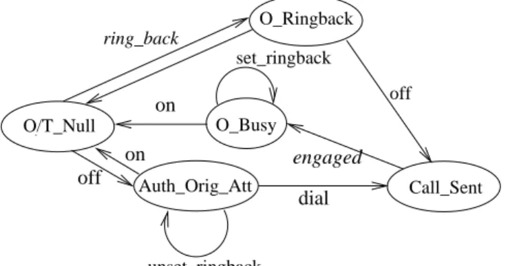
We do not give automata for all the features, but give only one example. Figure 3 illustrates the change in user-perceived behaviour when the user sub-scribes to the ring back when free feature (RBWF). Note that the set ringback
and unset ringback events correspond to the storing of the number of the sub-scriber’s current partner (within an array) so that a ringback to that number can subsequently be initiated. The automaton associated with RWF is similar, although the subscriber does not set (or unset) an array in the same way. In fact it is set by the originator of the call.
on ring_back off unset_ringback dial Call_Sent O_Ringback O/T_Null Auth_Orig_Att off on O_Busy set_ringback engaged
Figure3.Finite State Automaton for RBWF
8
The Features in Promela
We do not give all the details of the implementation of features in Promela, but draw attention to some of the more important aspects:
– To implement the features we have included a “feature lookup” function (see below) that implements the features and computes the transitive closure of the forwarding relations (when such features apply to the same call state).
– New feature arrays are included, namelyCFU,CFBetc. These are initialised within the init process according to which features are present within a given configuration. Note that the arrays associated with theRBWF,RWF,
OCO and TCO features contain 0s and 1s only. As SPINdoes not support bit arrays, these arrays are stored as arrays of bytes, using far more memory than necessary. Thus we could have saved valuable space by using bitvectors [52] rather than arrays in this case. However, for simplicity (in describing thefeature lookupbelow, for example) and consistency (with respect to the other features) we have used byte arrays.
– We distinguish between call and dial screening; the former means a call between user A and B is prohibited, regardless of whether or not A actually dialed B, the latter means that if A dials B, then the call cannot proceed, but they might become connected by some other means. The latter case might be desirable if screening is motivated by billing. For example, if user A dials C (a local leg) and C forwards calls to B (a trunk leg) then A would only pay for the local leg.
– Currently we restrict the size of the lists of screened callers (relating to the OCS, ODS and TCS features) to one. That is, we assume that it is impossible for a single user to subscribe to two of the samescreening feature. This is sufficient to demonstrate some feature interactions, and limits the size of the state-space.
– The addition of either of the ringback features, RBWF or RWF, while straightforward, significantly increases the complexity of the underlying state-space. The reason for this is that an entirely new call state (O Ringback) must be included in each case. In addition an array,rgbknumandretnum respec-tively, must be included to record the last process to whom a ringback has been initiated. The issue is not just that there is a new global variable, but thatcallstates that were previously identified are now distinguished by the contents of these arrays (c.f. discussion above about variable reinitialisation).
– To ensure that all variables are initialised, we again use 6 as a default value (assuming that the total number of users is 4). This is particularly useful when a user does not subscribe to a particular feature. The value 7 is used to denote both an unobtainable number (e.g. an incorrect number) and to denote “cancel ringback” in RBWF. We do not use an additional value for the latter, so as not to increase the size of the state-space.
8.1 Implementation of Features: the feature lookupinline
In order to enable us to add features easily, all of the code relating to feature behaviour is now included within an inline definition, as follows.
inline feature_lookup(q1,id1,st) { do ::((id1!=7)&&(st==st_dial)&&(CFU[id1]!=6)) -> id1=CFU[id1];q1=chan_name[id1] ::((id1!=7)&&(st==st_dial)&&(CFB[id1]!=6)&&(len(q1)>0)) -> id1=CFB[id1];q1=chan_name[id1] ::((st==st_dial)&&(ODS[selfid]==id1)) -> st=st_unobt ::((st==st_call2)&&(OCS[selfid]==id1)) -> st=st_unobt ::((st==st_call2)&&(TCS[id1]==selfid)) -> st=st_unobt ::((st==st_dial)&&(RBWF[selfid]==1)&&(id1==7)&&(rgbknum[selfid]!=6)) -> rgbknum[selfid]=6;st=st_redial ::((st==st_idle)&&(RBWF[selfid]==1)&&(rgbknum[selfid]!=6)&& (len(chan_name[rgbknum[selfid]])==0)) -> st=st_rback1 ::((st==st_rback2)&&(RBWF[selfid]==1)&&(rgbknum[selfid]!=6)) -> if
::dev=off;id1=rgbknum[selfid];q1=chan_name[id1]; rgbknum[selfid]=6;st=st_call1
::/*fail to respond to ringback tone*/
self?messchan,messbit; assert(messchan==self); messchan=null; messbit=0;rgbknum[selfid]=6;st=st_preidle fi ::((st==st_busy)&&(RBWF[selfid]==1)&&(rback_flag==0)&&(id1!=selfid)) -> if ::rgbknum[selfid]=id1 ::skip fi; rback_flag=1 ::((st==st_idle)&&(RWF[selfid]==1)&&(retnum[selfid]!=6)&& (len(chan_name[retnum[selfid]])==0)) -> st=st_rback1 ::((st==st_rback2)&&(RWF[selfid]==1)&&(retnum[selfid]!=6)) -> if ::dev=off;id1=retnum[selfid];q1=chan_name[id1]; retnum[selfid]=6;st=st_call1
::/*fail to respond to ringback tone*/
self?messchan,messbit; assert(messchan==self); messchan=null; messbit=0;retnum[selfid]=6;st=st_preidle fi
::((st==st_busy)&&(RWF[id1]==1)&&(ret_flag==0)&&(id1!=selfid)) -> retnum[id1]=selfid; network_ev_action(ret_alert); ret_flag=1 ::((st==st_call2)&&(OCO[id1]==1)) -> st=st_unobt ::((st==st_idle)&&(TCO[selfid]==1)) -> st=st_blocked :: else ->break od }
The parametersq1,id1, andsttake the values of the current partner, partnerid and state of a user when a call to thefeature lookupinline is made. Notice, for example, that st can take two values relating to the Call Sent state, st call1 andst call2. This is to differentiate between the statetowhich the process is to be directed on leaving the inline function and the state fromwhich the process has entered the inline function respectively. As there is no redirection necessary from the O Busy state when either of the ringback features are present, the
rback f lag andret f lagvariables have been introduced to prevent the relevant guards from remaining true after the corresponding transitions have taken place (that is, to prevent an infinite loop). Statements withinfeature lookuppertaining to features that are not currently active are automatically commented out (see section 10.2).
feature lookupencapsulates centralised intelligence about the state of calls i.e. it encapsulates what is known as single point call control. (INsupports both single and multiple point call control.) This greatly simplifies the detection of MU feature interactions. Although MU interactions can be detected in a distributed architecture, i.e. in a multiple point call control, the negotiation required between switches creates a huge and irrelevant (for our purposes) overhead. We therefore have single point call control.
We note that type I interaction detection is greatly facilitated by the form offeature lookup: the majority of such interactions can be found by examining
the nondeterminism of the guards. For example, we can immediately see that the first two guards overlap if the state isst dial and the process subscribes to both CFU and CFB.
8.2 Incorporating Features within the Promela Specification
In order to illustrate how combinations of features are incorporated into the specification, we use a specific example. Suppose that there are four users and two active features, namely CFU and TCS, where user 0 forwards to user 1 and user 2 screens calls from user 0.
Consider a specification of the basic call model (see section 3) to which the
feature lookupinline, feature arrays, thergbk num andret numarrays and the
O Ringbackstate have been added.
Firstly thefeature lookupinline is adapted so that all lines of code that do not correspond to either CFU or TCS are removed. Thus the feature lookup
inline becomes: inline feature_lookup(q1,id1,st) { do ::((id1!=7)&&(st==st_dial)&&(CFU[id1]!=6)) ->id1=CFU[id1];q1=chan_name[id1] ::((st==st_call2)&&(TCS[id1]==selfid))->st=st_unobt ::else->break od }
Secondly the CFU andTCS arrays are initialised thus:
CFU[0]=1; CFU[1]=6; CFU[2]=6; CFU[3]=6; TCS[0]=6; TCS[1]=6; TCS[2]=0; TCS[3]=6;
All references to other feature arrays are removed. Finally the entireO Ringback
state is removed, together with thergbk num andret num arrays and all refer-ences thereof, as neither ringback feature is present.
In fact, for any combination of features, such changes are made automatically using a Perl script to create a specification from a template file (see section 10.2).
9
Temporal Properties for Features
The properties for features are more difficult to express than those for the ba-sic service. In order to reflect accurately the behaviour of each feature, great attention must be paid to the scopeof each property within the corresponding LTL formula, as described in section 5.3 (see for example [14]). For example, in property 8, it is essential that (for the CFB feature to be invoked) the for-warding party has a full communication channel whilst the dialing party is in
the Auth Orig Att state. This can only be expressed by stating that the forward-ing party must have a full channel continuously between two states, the first of which must occur before the dialing party enters the Auth Orig Att state, and the secondafterthe dialing party emerges from the Auth Orig Attstate.
The properties are designed to reflect the expected behaviour ofour particu-lar specification. For example, we expect the forwarding features to be initiated
immediatelyupon dialing. Thus we do not anticipate a user being able to hang up before a (redirected) connection is attempted. Property 7 reflects this expec-tation.
For the forwarding features, we want to capture the notion of a call attempt being made from userito userj. We can not insist that a connection is achieved as the line may be busy. In previous work [4] it was deemed sufficient that
partner[i] is set to chan name[j]. But, this does not completely capture the no-tion, with the consequence that we may miss some interactions (see section 10.4). Here we use the proposition below to represent the statement:a call attempt is made from user i to user j
(partner[i] ==chan name[j])
&& ((U ser[proci]@O Busy)||(U ser[proci]@O Alerting)).
We use the shorthandatt(i, j) to represent this proposition.
In some of the properties, propositions relate to the value of a variable (dialed[i] say). It is often necessary to refer to the value of a variableat a particu-lar point in the service. For example, in property 7 we are interested in cases when the value of the variabledialed[i] is j when processi is at the Call Sentstate. (The value ofdialed[i] may be equal to jat a later state,O No Answersay, by which time it is too late to determine whetherprocess[i] subsequently attempts a call to the new partner.) Hence we enhance the proposition dialed[i] == j
with the extra condition that (U ser[proci]@Call Sent).
In section 5.2 we discuss the use of @ statements and event variables to track the progress of a process. The particular property dictates which of these to use. However, sometimes great caution must be exercised. For example, it is tempting to replace propositionatt(i, j) with the propositionnew att(i, j) below:
(partner[i] ==chan name[j])
&& ((network event[i] ==engaged)||(network event[i] ==oring)).
However,network event[i] only takes the valueengaged(or, at least, it is only visible to thenever-claimas such) afterprocess[i] leaves the O Busystate and proceeds to the P reidlestate, by which time partner[i] has been reset to the default value ofnull. Thus it is essential that an @ statement is used here. As far as possible the properties either use @ statements throughout or event variables. This is because the use of both would increase the number of variables that would be required, which would increase the size of the resulting state-space unnecessarily. Unfortunately, for the properties associated with the ringback features it is necessary to use both types of statement in order to fully express the desired behaviour.
Some of the properties below refer to the status of the device associated with a process. That is they refer to the device beingonoroff. In order to make this visible to the never-claim, the local variable dev must be replaced throughout the corresponding model by a global array ofdevvariables.
We have been especially careful to avoid theandX(next-time) operators in our properties. Both of these operators carry an increase in the cost of verification (due to the necessity of adding theweak fairnessconstraint and the prohibition of the use of partial order reduction respectively, see section 2.5). Sometimes the use of these operators is essential. However, we have managed to avoid their use in this instance, via judicious use of theU operator.
In each property the values of the variablesi, jandkdepend on theparticular pair of features and the corresponding property that is being analysed. These variables are therefore updated prior to each verification either manually (by editing the Promela code directly), or automatically during the running of a specification-generating script (see section 10.2).
Property 7 – CFUAssume that user j forwards to k.
If user i rings user j then a connection between i and k will be attempted before user i hangs up.
LTL: [](p→(rPq))
p= ((dialed[i] ==j)&&(U ser[proci]@Call Sent)),r=att(i, k),
q= (dev[i] ==on).
Property 8(a) – CFBAssume that user j forwards to k.
If user i rings user j when j is busy then a connection between i and k will be attempted before user i hangs up.
LTL: [](((u∧t)∧((u∧t)U((¬u)∧t∧p)))→(rPq))
p= ((dialed[i] ==j)&&(U ser[proci]@Call Sent)),t= (full(chan name[j])),r
=att(i, k),u= (U ser[proci]@Auth Orig Att),
q= (dev[i] ==on).
Property 8(b) – CFB Assume that user j forwards to k.
If user i rings user j when j is not busy then a connection between i and j will be attempted before user i hangs up.
LTL: [](((u∧t)∧((u∧t)U((¬u)∧t∧p)))→(rPq))
p= ((dialed[i] ==j)&&(U ser[proci]@Call Sent)),t= (empty(chan name[j])),
r=att(i, j),u= (U ser[proci]@Auth Orig Att),q= (dev[i] ==on).
No connection from user i to user j is possible. LTL: [](¬p)
p= (connect[i].to[j] == 1).
Property 10 – ODSAssume that user i has user j on its screening list,i=j.
User i may not dial user j. LTL: [](¬p)
p= (dialed[i] ==j).
Property 11 – TCSAssume that user i has user j on its screening list,i=j.
No connection from user j to user i is possible. LTL: [](¬p)
p= (connect[j].to[i] == 1).
Property 12 – RBWFAssume that user i has RBWF.
If user i has requested a ringback to user j (i=j) (and not subsequently requested a ringback to another user) and subsequently user i is at O/T Null when users i and j are both free, (and they are still free when user i is no longer at O/T Null) then user i will hear the ringback tone.
LTL: []¬((p&&q&&r&&s)&&((p&&q&&r&&s)U((p&&(¬q)&&r)&&((¬t)U q))))
p= (rgbknum[i] ==j),s= (len(chan name[i]) == 0),
q= (U ser[proci]@O/T N ull),r= (len(chan name[j]) == 0),
t = (network event[i] ==ringbackev).
Property 13 – OCOAssume that user j has OCO.
No connection from user i to user j is possible. LTL: [](¬p)
p= (connect[i].to[j] == 1).
Property 14 – TCOAssume that user j has TCO.
No connection from user j to user i is possible. LTL: [](¬p)
Property 15(a) – RWFAssume that user j has RWF.
If user i calls user j when user j is busy (i=j), then user i will hear the ret alert tone andretnum[i]will be set toj(before user i returns to the O/T Null state). LTL: []¬((p&&q&&v)&&((p&&q&&v)U(p&&v&&(¬q)))&&((¬(r&&s))U(t)))
p= (len(chan name[j])>0),q= (U ser[proci]@O Busy),
v = (partner[i] ==chan name[j]),t=(U ser[proci]@O/T N ull),
r= (retnum[j] ==i),
s= (network event[i] ==ret alert).
Property 15(b) – RWFAssume that user j has RWF.
If user i has requested a ringback from user j (i=j) (and subsequently no other user has requested a ringback from user j), and user j is at O/T Null and and users i and j are both free, then user j will hear the ringback tone.
LTL: []¬((p&&q&&r&&s)&&((p&&q&&r&&s)U((p&&(¬q)&&r)&&((¬t)U q))))
p= (retnum[j] ==i),s= (len(chan name[i]) == 0),
q= (U ser[procj]@O/T N ull),r= (len(chan name[j]) == 0),
t = (network event[j] ==ringbackev).
10
Feature Interaction
In this section we consider only systems of 4 processes. Generalisation is discussed in section 11.
A property based approach to feature interaction detection assumes a formal model of the entire system and a given set of properties (usually temporal) associated with the features. In our case the formal model is the underlying Kripke structure associated with the Promela specification (see section 2.3).
Two features are said tointeractif a property that holds for the system when only one of the features is present, does not hold when both features are present. For featuresf1andf2we define feature interaction as follows:
Definition 2. Let M be the model of a system of N components in which no features are present and let M(f1),M(f2) andM(f1∩f2)be models in which onlyf1, onlyf2and bothf1andf2have been added respectively. Ifφ1andφ2are properties that define f1 andf2 respectively then f1 and f2 are said to interact if
M(f1)|=φ1but M(f1∩f2)|=φ1, or
M(f2)|=φ2but M(f1∩f2)|=φ2.
Note that this definition is relatively high-level, it does not contain details of the configuration. Thus it does not distinguish between SC (single component) and MC (multiple component) interactions. When we report on results later
(section 10.3) we will make this distinction. Note also that this analysis will only reveal interactions that exist with respect to the particular properties φ1 and
φ2. For complete analysis it may be necessary to perform analysis for a suite of properties for each feature, or to conjoin properties.
10.1 Feature Validation
Before we can perform pairwise analysis of features, we must ensure that, for any feature, the model containing that feature in isolation satisfies the associated feature property. That is, using the notation above, we must show that for any featuref with associated property φ, M(f)|=φ.
Features and properties are labelled according to table 2. Each property must be checked for all relevant values ofiandj (andkif appropriate).
Table2.Features and properties
Feature Propertyφ CFU property 7
CFB (property 8a) && (property 8b) OCS property 9 ODS property 10 TCS property 11 RBWF property 12 OCO property 13 TCO property 14
RWF (property 15a) && (property 15b)
Exploiting Symmetry A brute force approach quickly suffers a combinatorial explosion. For example, to verify property 7 (for all suitable networks of pro-cesses) with only four users, we need to check 48 cases (4 choices foriandj and 3 choices fork). We can eliminate the need to consider all cases by appealing to symmetry.
Consider the simplest case, wherei,j, andk are distinct. Any permutation
σ takingi, j and kto distincti,j andk will preserve the transition relation of the underlying Kripke structure. The two models will be bisimilar and hence satisfy the same LTL formula, provided the formula is suitably renamed under
σ. More formally, letMbe a Kripke structure,sa state andφan LTL formula involving onlyi,j, andk-indexed propositions, andσa permutation withMσ,
σs and σφ the appropriate transformations under σ. There is a bisimulation betweenMandMσ and so we have:
The proof follows from the result that CTL* is adequate with respect to bisimu-lation [2]. This result relating permutations is similar, yet different to the result for symmetry groups and CTL* formulae [11]. The formulae, besides being in LTL (rather than CTL*), must be transformed under σ, unlike the symmetry group result where it may not be transformed and must be invariant under all permutations. This is because the symmetry group result is over the quo-tient structure, rather than individual (unquoquo-tiented) structures. We consider the individual structures and the permuted properties because our motivation is different: we require to reduce the number of cases to model check, not the state-space.
Application of this result allows us to exclude from consideration permuta-tions of most of the relevant properties. For example, for property 7 we need consider only 3 cases (i= 0, j= 0, k= 1;i= 1, j= 0, k= 1;i= 2, j= 0, k= 1). All other cases are just a permutation of one of these.
Feature Validation Results For every featuref, associated propertyφ and choice of parameters, a Promela specification was constructed and verified. In each case the property was satisfied.
Clearly it is not possible to give detailed results for each relevant pair of features and properties. However in table 3 we give detailed verification results for each property for an example configuration of (distinct) parametersi,j(and
k), when checked against a suitable network of processes.
Table3.Verification Results – feature properties
Property Depth (×106) States (×105) Mem Time state-vector
7 0.6 3.0 12.6 15 116 8a 1.4 9.4 36.8 43 116 8b 1.4 7.9 32.7 40 116 9 1.2 6.1 23.8 29 124 10 1.1 6.4 25.4 30 136 11 1.1 6.3 25.1 29 136 12 11.2 59.5 263.7 385 132 13 0.6 3.1 13.0 16 136 14 0.5 3.2 12.9 16 136 15(a) 12.4 67 296.3 438 132 15(b) 12.3 70.2 308.7 476 132 10.2 Interaction Analysis
We now consider the case where two features are present. That is, we consider networks of 4 processes in which features f1 and f2 are present and determine