(will be inserted by the editor)
Rejoinder to ‘Multivariate Functional Outlier Detection’
Mia Hubert · Peter Rousseeuw · Pieter Segaert
Received: date / Accepted: date
First of all we would like to thank the editor, Professor Andrea Cerioli, for inviting us to submit our work and for requesting comments from some esteemed colleagues. We were surprised by the number of invited comments and grateful to their contribut-ing authors, all of whom raised important points and/or offered valuable suggestions. We are happy for the opportunity to rejoin the discussion. Rather than addressing the comments in turn we will organize our rejoinder by topic, starting with comments directly related to concepts we proposed in the paper and continuing with some ex-tensions.
1 Bagdistance and bagplot
We did not know that the name ‘bagdistance’ was already used in a totally different setting, as pointed out by Karl Mosler. We sort of assumed that the name ‘bagdis-tance’ sounded strange enough to be unique, but we will be careful to consult Dr. Google next time!
More importantly, we were not aware of the paper by Riani and Zani (1998) that was referenced in the discussion by Aldo Corbellini, Marco Riani and Anthony Atkinson. That paper appeared in the proceedings of a conference neither of us at-tended, and unfortunately it is much harder to look up an idea by search engine than it is to look up a phrase. In the meantime the authors were so kind as to provide us with a copy of their paper. We agree that the generalized distance of Riani and Zani (1998) is very similar to the bagdistance for p62, the only difference being the choice of contour (in their case based on elliptical peeling and cubic spline smooth-ing) and center (for which they use the intersection of two least squares lines). As their construction was restricted to p=2 they extended it to higher dimensions by
M. Hubert, P. Rousseeuw, P. Segaert
Department of Mathematics, KU Leuven, Celestijnenlaan 200B, BE-3001 Heverlee, Belgium Tel.: +32-16-322023
applying their method to pairs of variables. The generalized distance of Riani and Zani (1998) has many aspects in common with the bagdistance, such as its ability to reflect asymmetry in the data.
We still prefer the bag and center based on halfspace depth, because halfspace depth is more robust than convex peeling as shown by Donoho and Gasko (1992) and the definition of the bagdistance applies to any dimension. As an aside, the bag as de-fined in Rousseeuw et al. (1999) was interpolated between two depth contours, so no data point had to lie on the contour of the bag. However, some simplified algorithms for the bag do have this property.
Riani and Zani (1998) explicitly draw thefence(the boundary outside of which points are flagged as outlying) in their plot, at the distanceqχ22,0.99 which almost
exactly coincides with the factor 3 of the bagplot’s fence. The bagplot shows the loop, which is the convex hull of the data points inside the fence and generalizes the whiskers of the univariate bagplot. By default the bagplot doesn’t show the fence itself, but we included it in Figure 1(a) for comparison. It is a plot of plasma triglyc-eride concentration versus cholesterol forn=320 patients (Hand et al. 1994) with pronounced skewness.
2 Hubert, Rousseeuw, Segaert
0 250 500 750 1000 100 200 300 400 Cholesterol T riglycer ides
Bagplot based on halfspace depth
Fig. 1Bagplot of the bloodfat data based on
halfs-pace depth with indication of the fence.
0 250 500 750 1000 100 200 300 400 Cholesterol T riglycer ides
Bagplot based on skew−adjusted projection depth
Fig. 2 Bagplot of the bloodfat data based on
skew-adjusted projection depth with indication of the fence.
Box-cox transformation: eventueel verwijzen naar Yohai, Van der Veeken (wordt misschien al teveel, we verwijzen al een keer naar Riani)
3 Weight function
In our examples we always used a constant weight function in MFD, but as already explained in Claeskens et al (2014) using a non-constant weight function can be very interesting if we want to emphasize or downweight certain time periods. Usually the data do not come with their own intrinsic weight function, so this is a choice of the statistician depending on the purpose of the study. As pointed out by? this choice might heavily affect the conclusions, so a well-chosen weight function is indispens-able. When the purpose is on outlier detection,?propose to use a weight function which is proportional to the variability of the curves. Instead of a robust measure of variability (such as the volume of the depth regions proposed in Claeskens et al (2014)) they consider a non-robust measure.
[Mia: ik ga nog proberen een figuur te maken waarbij dit hopelijk misgaat...] Extending the functional bagdistance and adjusted outlyingness with a weight function is a valuable suggestion. [dan misschien zeggen dat we fbd en fAO altijd bedoeld hadden met kansmaat erbij? Ligt lastig, maar we moeten er wel iets over zeggen voor we de FOM van volgende sectie kunnen invoeren].
4 Functional outlier map
Several good ideas concerning Centrality-stability plot: to rescale the vertical axis (He), to focus on the outlyingness instead of centrality (Alicia, Genton), to put the standard deviation of the AO on the vertical axis (Alicia). Combining the ideas leads to our new proposal of functional outlier map:stdt(AO)/(1+f AO)on vertical axis,
and fAO on the horizontal axis. And size of the bullet according to percentage of time it is declared as a multivariate outlier, to reflect the amount of local outlyingness. If
Fig. 1 Bloodfat data: (a) bagplot based on bagdistance; (b) bagplot based on adjusted outlyingness. In
both cases the dashed line is the fence.
Note that we can also create ‘generalized bagplots’ based on other distance mea-sures than the bagdistance. For instance, we can use the skew-adjusted outlyingness AO which is even more robust than halfspace depth. Since we showed in Theorem 4 that its contours are convex, the resulting generalized bagdistance is a norm. Gener-alizing the fence of the bagplot we could flag ap-variate pointxas outlying if
AO(x)/median
i (AO(xi))>
q
χ2p,0.99
Figure 1(b) shows the bagplot based on AO with this cutoff. It looks similar to that based on halfspace depth, but is not quite the same. Several points at the bottom of the plot used to be barely inside the fence, and are now barely outside. Fortunately, in a graphical display it is easy to see that they are borderline cases.
Note that the above formula for the cutoff is similar to that of the usual Ma-halanobis distance, whose distribution can be approximated byχp1under normality.
Therefore, the above cutoff shares the ‘curse of dimensionality’ issues of the Maha-lanobis distance for highp, such as the fact that its distribution gets concentrated at its median. In other words, clean normal observations lie essentially on a sphere with very few points inside of it. Therefore, we only use this cutoff for smallp.
2 Weight function
The examples in the paper used a constant weight function in MFD, but as already explained by Claeskens et al. (2014) a non-constant weight function can be very use-ful to emphasize or downweight certain time periods. We will always assume w.l.o.g. that the discrete weights sum to one (and analogously that the weight function inte-grates to one), which has the advantage that e.g. the functional adjusted outlyingness fAO is on the same scale as the AO at one time point.
Usually the data do not come with their own intrinsic weight function, so this is a choice of the statistician depending on the purpose of the study. As pointed out by Francesca Ieva and Anna Paganoni, this choice might heavily affect the conclusions, so a well-chosen weight function is indispensable. When the purpose is to detect out-liers, Davy Paindaveine and Germain Van Bever propose to use a weight function which is proportional to the variability of the curves. Instead of a robust measure of variability [such as the volume of the depth regions proposed in (Claeskens et al. 2014)] they prefer a nonrobust measure for this purpose. Alternatively, the weight function could be the inverse of a robust dispersion meausure. Sara L´opez suggested to extend the functional bagdistance and adjusted outlyingness as well by incorporat-ing a weight function.
3 Functional outlier map
Several discussants provided good ideas concerning the centrality-stability plot. Naveen Narisetti and Xuming He proposed to standardize the quantity on the vertical axis in order to stabilize its variability. Yuan Yan and Marc Genton, as well as Alicia Nieto-Reyes and Juan Cuesta-Albertos, suggested to focus on outlyingness instead of centrality, and the latter discussants also proposed to put the standard deviation of the AO on the vertical axis instead of the formula with the harmonic mean. We are grateful for these insightful suggestions. Combining these ideas leads to a new proposal for afunctional outlier map, which is to plot for each curveYiits fAO(Yi;Pn)
(the functional AO) on the horizontal axis and stdev
j (AO(Yi(tj);Pn(tj)))/(1+fAO(Yi;Pn))
on the vertical axis. This outlier map can then be read in a way similar to the outlier map of robust regression (Rousseeuw and van Zomeren 1990) and the outlier map of robust principal components (Hubert et al. 2005).
The division by fAO on the vertical axis can be justified as follows. Suppose the center curve is at zero, andYk(t) =2Yi(t)in allt. Then stdevj(AO(Yk(tj);Pn(tj))) =
2 stdevj(AO(Yi(tj);Pn(tj)))as well as fAO(Yk;Pn) =2 fAO(Yi;Pn)while their relative
variability is the same.
According to the previous section, both fAO(Yi;Pn) =avej(AO(Yi(tj);Pn(tj)))
and stdevj(AO(Yi(tj);Pn(tj))) in the above formula can be weighted using a time
weight.
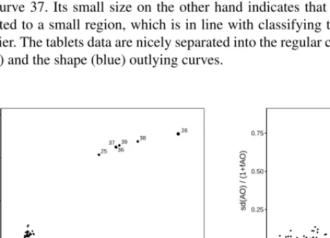
We have added one more feature to the map. The points are plotted as ‘bub-bles’, with the size of the bubble representing the fraction of the time the function is flagged as a multivariate outlier. This reflects the amount of local outlyingness. Figure 2 shows the resulting outlier maps for the four examples studied in the paper. The outlier map of the wine data immediately shows the high degree of outlyingness of curve 37. Its small size on the other hand indicates that its outlying behavior is limited to a small region, which is in line with classifying this curve as an isolated outlier. The tablets data are nicely separated into the regular curves (orange), the shift (red) and the shape (blue) outlying curves.
Rejoinder to ‘Multivariate Functional Outlier Detection’ 3
proportion is at most 25%, then size of point is smallest; at most 50% then size is second smallest and so on.
Difficult to define cutoff values (Lopez). Idea of signed AO does not seem to work well (and refer to compstat paper of Hubert-VdV (2010) for the definition of signed AO). [ook het niet-werkende voorbeeld van tablets data tonen?]
25 26 36 37 39 38 0.0 0.5 1.0 1.5 0 5 10 15 fAO sd(A O) / (1+fA O) 2 3 23 35 37 0.00 0.25 0.50 0.75 1.0 1.5 2.0 2.5 fAO sd(A O) / (1+fA O) 30 41 67 95 121 132 0.0 0.1 0.2 0.3 1.5 2.0 2.5 3.0 fAO sd(A O) / (1+fA O) 0.1 0.2 0.3 0.4 2 3 4 5 6 fAO sd(A O) / (1+fA O)
Fig. 3 Functional outlier map of the Octane, Wine, Writing and Tablets data.
5 Computation
We are intrigued by the example given by Alicia (large dimensions and still possible to find the outliers by using only 20 random directions. In contradiction with Mosler (instability of the projection depth). Interesting for further research. Current example is not fully convincing as we also find the outliers based on their Euclidean norm, by considering the directions through the mean and each data point (apart from obs 7) [dus dit misschien niet vermelden?]. And the AO based on 20 random directions also finds them easily, as can be seen on the heatmap in Figure 4 and the functional outlier map in Figure 5.
Fig. 2 Functional outlier map of the Octane, Wine, Writing and Tablets data.
The univariate signed AO suggested by Naveen Narisetti and Xuming He was previously defined by Hubert and Van der Veeken (2010, page 1137). It indeed works well for univariate functions (p=1), but we found its multivariate generalization to be rather unstable to small changes in the functional data. Therefore, in the above
functional outlier map we chose to stick with the unsigned AO in order to keep the same definition for allp.
It would be great if we could improve the functional outlier map by drawing vertical and horizontal cutoff lines based on some simple quantiles. However, such cutoffs have to depend on the autocorrelation of the observed functions, as explained in the contribution of Yuan Yan and Marc Genton who reference the interesting papers of Sun and Genton (2011, 2012) where this technology was developed.
4 Computation
The examples in our paper had low dimensionp, but of course we want to be able to deal with high dimensions as well. About this the discussants were not all in agree-ment. Karl Mosler felt that the projection depth (and thus also the SDO, SPD, and AO) requires projecting the data on a huge number of directions, in fact exponential inp. Alicia Nieto-Reyes and Juan Cuesta-Albertos voiced the opposite opinion, that a small number of random directions is sufficient to compute the random Tukey depth, and illustrated this on a generated data set in 200 dimensions, withn=39 curves containing 7 outliers. They drew 20 directions from the uniform distribution on the sphere and found all the outliers. It seems to us that when the random Tukey depth works, so should the adjusted outlyingness AO. Alicia and Juan were kind enough to provide their data, so we also generated 20 such random directions and computed the AO in each projection. This again found all the outliers, as can be seen in Figure 3(a). Figure 3(a) looks a bit different from the heatmap shown by the discussants, which is only because we added a feature to this graphical display. By default, the shading in the heatmap is directly proportional to the AO, which ranges from zero to its maximal value. This is not robust however, since large values of AO could be masked by one extremely large value. Therefore, going forward we assign the darkest shading to all AO that exceed a certain value, in this case 40. (Mechanically, this is done by truncating the AO values in the call to the heatmap function.) This way we can see all the outliers in one heatmap.
Figure 3(b) shows the functional outlier map of these data. Curves 2 and 4 have the largest fAO because they are outlying in every dimension, and have the largest bubbles. Curve 5 has the largest variability as it has a huge AO at a few time points and a small AO at all other times, so it stands out as an isolated outlier. Curve 7 lies close to the regular data, in accordance with how it was generated.
So, how can we reconcile the viewpoints of Karl Mosler with those of Alicia Nieto-Reyes and Juan Cuesta-Albertos? We think the difference is mainly caused by the type of invariance these authors aim for. Karl sits squarely in the camp of affine invariance, so he will typically compute directions orthogonal to random p -subsets, and as in all algorithms of this type it takes an exponential number of draws to reach the desired probability of a cleanp-subset. Alicia and Juan aim for orthogonal invariance instead, even though they do not say so explicitly. Their method is not affine invariant since an affine transform can map the uniform distribution on the sphere to a very different distribution. However, an orthogonal transformation does leave the uniform distribution unchanged.
10 18 11 14 24 34 37 38 23 12 28 17 25 36 39 20 30 8 16 9 13 35 27 15 29 32 33 31 26 21 22 19 7 5 3 6 1 4 2 1 33 65 97 129 161 193 225 wavelength 10 20 30 40+ AO 1 2 3 4 5 6 7 1 2 3 4 0 10 20 30 40 fAO sd(A O) / (1+fA O) 18 23 17 22 8 35 27 20 39 15 25 12 9 14 30 21 3 19 34 33 31 32 13 38 36 24 1 29 28 37 16 11 26 5 7 10 6 4 2 1 33 65 97 129 161 193 225 wavelength 10 20 30 40+ AO 22 18 12 9 8 17 39 25 15 11 33 20 26 14 34 24 35 36 28 7 23 6 16 27 21 5 19 13 31 1 3 37 10 30 38 29 32 4 2 1 33 65 97 129 161 193 225 wavelength 10 20 30 40+ AO
with local depth and bagdistances in the multivariate space of the observations, and give a nice graphical illustration.
6 Images
Sara L´opez as well as Yuan Yan and Marc Genton mention the possibility to extend our work to situations where the index is no longer univariate (like time or wave-length) but bivariate, as in the case of surfaces or images. A very nice depth-based exploratory tool to analyze image data has been proposed in Genton et al (2014) by generalizing the band depth to volume depth.
Multivariate functional depth and our new outlier detection tools also easily gen-eralize to surfaces and images. We illustrate this on the Dorrit data, previously ana-lyzed in Engelen et al. (2007), Engelen and Hubert (2011) and Hubert et al. (2012). This data set contains excitation-emission (EEM) landscapes of 27 mixtures of four known fluorophores with excitation wavelengths ranging from 230 nm to 315 nm ev-ery 5 nm, and emission at wavelengths from 250 nm to 482 nm at 2 nm intervals.
Hence each sampleYicontains 18×116 measurementsYi(j,k)for j=1, . . .J=18
andk=1, . . . ,K=116.
Fig. 3 200-dimensional data set of Nieto-Reyes and Cuesta-Albertos. Top row: (a) AO heatmap based on
20 random directions; (b) functional outlier map. Bottom row, after affine transformation of the data: (c) heatmap based on 20 random directions; (d) heatmap based on 500 random directions.
To verify this explanation we wrote some code to generate a random affine trans-formation. After applying this to the 200-dimensional dataset and projecting on the same 20 random directions as before, yielding the heatmap in Figure 3(c), we only detect outliers 2 and 4 which are outlying in every dimension, whereas the other out-liers remain hidden. This is still true if we draw 500 random directions, as seen in Figure 3(d).
5 Local outlyingness
Several people have commented on local outlyingness, where a function is outlying only on a small time interval. Karl Mosler proposes an approach which divides the time interval into subintervals. Luis-Angel Garc´ıa-Escudero, Alfonso Gordaliza, and Agostin Mayo-Iscar note that isolated outliers correspond to cellwise outliers in the terminology of Alqallaf et al. (2009). In the case of functional data, they offer an identification technique based on local trimming. Both discussions as well as that of Francesca Ieva and Anna Paganoni also bring up the connection between outlier detection and supervised classification (clustering). Davy Paindaveine and Germain Van Bever are concerned with local depth and bagdistances in the multivariate space of the observations, and give a nice graphical illustration.
6 Images
Sara L´opez-Pintado as well as Yuan Yan and Marc Genton mention the possibility to extend our work to situations where the index is no longer univariate (like time or wavelength) but bivariate, as in the case of surfaces or images. A very nice depth-based exploratory tool to analyze image data has been proposed in Genton et al. (2014) by generalizing the band depth to volume depth.
Multivariate functional depth and our new outlier detection tools also easily gen-eralize to surfaces and images. We illustrate this on the Dorrit data, previously ana-lyzed in Engelen et al. (2007), Engelen and Hubert (2011) and Hubert et al. (2012). This data set contains excitation-emission (EEM) landscapes of 27 mixtures of four known fluorophores with excitation wavelengths ranging from 230 nm to 315 nm ev-ery 5 nm, and emission at wavelengths from 250 nm to 482 nm at 2 nm intervals. Hence each sampleYicontains 18×116 measurementsYi(j,k)for j=1, . . . ,J=18
andk=1, . . . ,K=116.
The functional depth of landscapeYi(withi=1, . . . ,27) then becomes
MFD(Yi;Pn) = 18
∑
j=1 116∑
k=1 D(Yi(j,k);Pn(j,k))Wjkwith∑j∑kWjk=1. Similarly we define the functional adjusted outlyingness fAO as
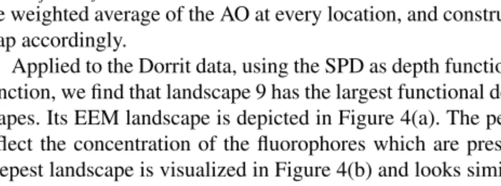
the weighted average of the AO at every location, and construct the functional outlier map accordingly.
Applied to the Dorrit data, using the SPD as depth function and a constant weight function, we find that landscape 9 has the largest functional depth among the 27 land-scapes. Its EEM landscape is depicted in Figure 4(a). The peaks in these landscapes reflect the concentration of the fluorophores which are present in the mixture. The deepest landscape is visualized in Figure 4(b) and looks similar but less smooth as it does not correspond to an observed surface.
6 Images
Sara L´opez as well as Yuan Yan and Marc Genton mention the possibility to extend our work to situations where the index is no longer univariate (like time or wave-length) but bivariate, as in the case of surfaces or images. A very nice depth-based exploratory tool to analyze image data has been proposed in Genton et al (2014) by generalizing the band depth to volume depth.
Multivariate functional depth and our new outlier detection tools also easily gen-eralize to surfaces and images. We illustrate this on the Dorrit data, previously ana-lyzed in Engelen et al. (2007), Engelen and Hubert (2011) and Hubert et al. (2012). This data set contains excitation-emission (EEM) landscapes of 27 mixtures of four known fluorophores with excitation wavelengths ranging from 230 nm to 315 nm ev-ery 5 nm, and emission at wavelengths from 250 nm to 482 nm at 2 nm intervals. Hence each sampleYi contains 18×116 measurementsYi(j,k)for j=1, . . .J=18 andk=1, . . . ,K=116.
The functional depth of landscapeYi(withi=1, . . . ,27) then becomes MFD(Yi;Pn) = 18
∑
j=1 116∑
k=1 D(Yi(j,k);Pn(j,k))Wjkwith∑j∑kWjk=1. Similarly we define the functional adjusted outlyingness fAO as the weighted average of the AO at every location, and construct the functional outlier map accordingly.
Applied to the Dorrit data, using the SPD as depth function and a constant weight function, we find that landscape 9 has the largest functional depth among the 27 land-scapes. Its EEM landscape is depicted in Figure 4(a). The peaks in these landscapes reflect the concentration of the fluorophores which are present in the mixture. The deepest landscape is visualised in Figure 4(b) and looks similar but less smooth as it does not correspond to an observed surface.
Fig. 4 EEM landscape of (a) the deepest sample 9, and (b) the functional median.
The functional outlier map is presented in Figure 5. We note that landscape 5 has the highest fAO with very variable AO values.
Fig. 4 Dorrit data: (a) EEM landscape of the deepest surface 9; (b) EEM landscape of the functional
median computed from the data.
The functional outlier map is presented in Figure 5. We note that landscape 5 has the highest fAO with very variable AO values.
1 2 3 4 5 10 14 15 0.1 0.2 0.3 0.4 0.5 1.5 2.0 2.5 3.0 3.5 fAO sd(A O) / (1+fA O)
Fig. 5 Functional outlier map of the Dorrit data.
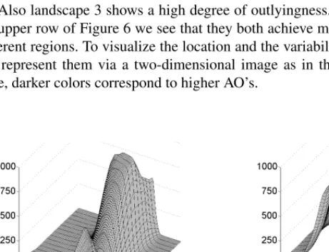
Also landscape 3 shows a high degree of outlyingness. From their raw values in the upper row of Figure 6 we see that they both achieve much larger values in many different regions. To visualize the location and the variability of these AO values we can represent them via a two-dimensional image as in the lower row of Figure 6. Here, darker colors correspond to higher AO’s.
Rejoinder to ‘Multivariate Functional Outlier Detection’ 9
230 240 250 260 270 280 290 300 310 250 300 350 400 450 Emission (nm) Excitation (nm) 0 4 10 15+ AO 230 240 250 260 270 280 290 300 310 250 300 350 400 450 Emission (nm) Excitation (nm) 0 4 10 15+ AO
Fig. 6Dorrit data: landscapes 3 and 5 (top row) with their two-dimensional AO values (bottom row). Genton MG, Johnson C, Potter K, Stenchikov G, Sun Y (2014) Surface boxplots. Stat
3:1–11.
Hand DJ, Daly F, Lunn AD, McConway KJ, Ostrowski E (1994) A Handbook of Small Data Sets. London: Chapman and Hall.
Hubert M, Van der Veeken S (2010) Fast and robust classifiers adjusted for skewness. Proceedings of COMPSTAT 2010, eds. Y. Lechevallier and G. Saporta, Physica-Verlag, pp. 1135–1142.
Hubert M, Van Kerckhoven J, Verdonck T (2012) Robust PARAFAC for incomplete data. Journal of Chemometrics 26:290–298.
Also here, the AO values exceeding a certain threshold (here 15) get the darkest color, so we can still make out the intermediate AO values. We see that landscape 3 is mostly outlying at the longer excitation wavelengths, whereas the outlyingness of landscape 5 is most prominent at the longer emission and the longer/shorter excitation wavelengths.
Note that in this exploratory analysis we only studied the differences between the landscapes based on their raw observed values. A more refined study could start by modeling the data through a parametric model (such as a PARAFAC model) and then apply our diagnostic tools to the residuals. Also two-dimensional warping and/or gradient functions could be added to improve performance.
References
1. Alqallaf F, Van Aelst S, Yohai VJ, Zamar RH (2009) Propagation of outliers in multivariate data. The Annals of Statistics 37:311–331
2. Claeskens G, Hubert M, Slaets L, Vakili K (2014) Multivariate functional halfs-pace depth. Journal of the American Statistical Association 109:411–423 3. Donoho D, Gasko G (1992) Breakdown properties of location estimates based on
halfspace depth and projected outlyingness. The Annals of Statistics 20:1803– 1827
4. Engelen S, Frosch Møller S, Hubert M (2007) Automatically identifying scat-ter in fluorescence data using robust techniques. Chemometrics and Intelligent Laboratory Systems 86:35–51
5. Engelen S, Hubert M (2011) Detecting outlying samples in a parallel factor anal-ysis model. Analytica Chimica Acta 705:155–165
6. Genton MG, Johnson C, Potter K, Stenchikov G, Sun Y (2014) Surface boxplots. Stat 3:1–11
7. Hand DJ, Daly F, Lunn AD, McConway KJ, Ostrowski E (1994) A Handbook of Small Data Sets. London: Chapman and Hall.
8. Hubert M, Rousseeuw PJ, Vanden Branden K (2005) ROBPCA: a new approach to robust principal components analysis. Technometrics, 47:64–79
9. Hubert M, Van der Veeken S (2010) Fast and robust classifiers adjusted for skew-ness. Proceedings of COMPSTAT 2010, eds. Y. Lechevallier and G. Saporta, Physica-Verlag, pp. 1135–1142
10. Hubert M, Van Kerckhoven J, Verdonck T (2012) Robust PARAFAC for incom-plete data. Journal of Chemometrics 26:290–298
11. Riani M, Zani S (1998) Generalized distance measures for asymmetric multivari-ate distributions. Advances in Data Science and Classification, eds. A. Rizzi, M. Vichi, and H.-H. Bock, Springer, pp. 503-508
12. Rousseeuw PJ, Ruts I, Tukey J (1999) The bagplot: a bivariate boxplot. The American Statistician 53:382–387
13. Rousseeuw PJ, van Zomeren BC (1990) Unmasking multivariate outliers and leverage points. Journal of the American Statistical Association 85:633–651 14. Sun Y, Genton MG (2011) Functional boxplots. Journal of Computational and
15. Sun Y, Genton MG (2012) Adjusted functional boxplots for spatio-temporal data visualization and outlier detection. Environmetrics 23:54–64