Joint Detection and Classification Convolutional Neural Network on Weakly Labelled Bird Audio Detection

Joint Detection and Classification Convolutional

Neural Network on Weakly Labelled Bird Audio

Detection

Qiuqiang Kong, Yong Xu, Mark D. Plumbley

Center for Vision, Speech and Signal Processing (CVSSP)

University of Surrey

{

q.kong, yong.xu, m.plumbley

}

@surrey.ac.uk

Abstract—Bird audio detection (BAD) aims to detect whether there is a bird call in an audio recording or not. One difficulty of this task is that the bird sound datasets areweakly labelled, that is only the presence or absence of a bird in a recording is known, without knowing when the birds call. We propose to apply joint detection and classification (JDC) model on the weakly labelled data(WLD) to detect and classify an audio clip at the same time. First, we apply VGG like convolutional neural network (CNN) on mel spectrogram as baseline. Then we propose a JDC-CNN model with VGG as a classifier and CNN as a detector. We report the denoising method including optimally-modified log-spectral amplitude (OM-LSA), median filter and spectral spectrogram will worse the classification accuracy on the contrary to previous work. JDC-CNN can predict the time stamps of the events from weakly labelled data, so is able to do sound event detection from WLD. We obtained area under curve (AUC) of 95.70% on the development data and 81.36% on the unseen evaluation data, which is nearly comparable to the baseline CNN model.

I. INTRODUCTION

Bird audio detection (BAD) aims to detect the presence or absence of bird calls in an audio recording. BAD is a

sound event detection (SED) task, which aims to identify all the audio events and their occurrence time in a mixed audio recording. BAD has many applications in environmental science, such as monitoring the density and the migration of birds in depopulated zone. SED has attracted many attentions in recent years [1, 2]. Recently, a bird sound dataset around 40 hours with annotated labels is published with a bird detection challenge [3]. This dataset provides us the opportunity to research how the deep neural networks (DNN) can perform on SED tasks compared to the success on the image classification [4] and speech recognition [5].

BAD has many difficulties. First, in an audio clip only the presence or the absence of birds is known but not knowing the time stamps of the bird calls and other sounds. We refer to this kind of data as weakly labelled data (WLD) [6]. In contrast, we refer to the data with frame level label asstrongly labelled data(SLD). In practice, labelling the audio clips at the frame level is time consuming and impractical. In compromise, the audio recordings are usually cut into small chunks such as 10 seconds. Each chunk is labelled either 1 or 0 representing the presence or absence of a bird call in this chunk. This reduces the labelling time as well as increases the accuracy of the labelling procedure because the border of the bird call and

non-bird sounds are often ambiguous. Second, the call patterns of different birds varies. For example, the call patterns of a cuckoo and a sparrow are different. Third, audio recordings are usually mixed with other sounds such as dogs’ barking, human speech, and background noise such as wind or rain. Some sounds are hard to distinguish from real birds such as whistling or a fake bird call imitated by a human. Furthermore, in some scenes the signal to noise ratio (SNR) is very low and the noise may even conceal the bird calls. Previous research shows denoising is important in BAD [3]. However our experimental results show denoising is not helpful when using CNNs or our proposed JDC-CNN model.

We organize the paper as follows. In Section 2 we introduce the related works. In Section 3 we introduce audio denoising method applied in this paper. In Section 4 we propose a VGG convolutional neural network (CNN) on the mel spectrogram as a baseline CNN model. In Section 5 we proposea joint detection and classification (JDC-CNN) model. In Section 6 are show experimental results. Finally we summary our work and forecast the future work in Section 7.

II. RELATED WORKS

Bird audio detection (BAD) has attracted a range of interests since recent years. Early researches of BAD applies automatic speech recognition (ASR) techniques such as Gaussian mix-ture model (GMM) or hidden Markov model (HMM) [7, 8, 9] where mel spectrum or mel frequency cepstrum coefficient (MFCC) are usually used as features. MFCC is shown worse than mel spectrum on the bird detection task in [10]. In [10] spherical k-means and random forest algorithm are applied. Spherical k-means uses cosine distance instead of Euclidean distance so is robust to the energy dynamic change.

To use the weakly labelled data (WLD), multi instance learning (MIL) is applied in [11, 12]. In MIL the classification is on thebagsinstead of on theinstances(frames) where each bag is a collection of several instances (frames). A positive bag contains at least one positive instance while a negative bag consists of only negative instances.

Recently deep neural network methods such as convo-lutional neural networks (CNNs) [4] especially VGG nets [13] have been widely applied to image classification, speech recognition [5] and audio tagging [14]. Furthermore, we refer to [3, 15] as review papers of BAD.

mel spectrogram 440×40 + BN Conv 3×3, 32 fmaps, relu Conv 3×3, 32 fmaps, relu Maxpooling 2×1 + Dropout (0.25)

Conv 3×3, 64 fmaps, relu

Fig. 1. Baseline CNN [13] and joint detection and classification (JDC) model. Solid blocks are baseline CNN. Dash blocks together with solid blocks consist JDC-CNN model. Input is mel spectrogram with 440 frames and 40 mel frequency bins. Batch normalization is applied on each frequency bin.

The datasets of BAD task includes Warblr [3], Chernoby1 Exculusion Zone (CEZ) [3], Freefield [16], HJA [12], Bird-CLEF [17]. Most of the datasets are weakly labelled with only the presence or the absence of a bird in a recording but without frame level label.

III. CONVOLUTIONAL NEURAL NETWORKS

Convolutional neural networks (CNNs) have many suc-cessful applications in image related tasks, such as image classification [4] and object detection [18]. Compared to fully connected (FC) neural networks, CNNs have much fewer connections and parameters so they are easier to train and go deep. Recently CNNs have been applied to speech recognition [5] and audio tagging [14], where the spectrogram is fed to the CNN instead of using manual selected features such as Mel frequency coefficient cepstrum (MFCC) [19]. Recently a kind of CNN called VGG with small kernel size of 3×3 is proposed in [13] and is widely used in image classification [20]. In this paper we apply VGG on the mel spectrogram as a baseline CNN model (Figure 1).

IV. JOINT DETECTION AND CLASSIFICATION(JDC)MODEL

One deficiency of the baseline CNN is that the baseline CNN does not indicate when a sound event occurs. This is because the global max pooling or global average pooling in CNN does not preserve the local information of the feature maps. Global max pooling only uses the maximum value of each feature map and ignore other values. In contrast, global average pooling averages all values in a feature map even if some parts of a feature map does not contain events. Ideally we hope to find a pooling strategy utilizing all the values from

Fig. 2. JDC-CNN model. The detector decides whether to attend or ignore a frame. The classifier outputs a probability indicating a frame contains a bird call or other events. Fully connected classifier is built on the multiplication of the detector and the classifier.

the feature maps containing bird events and ignore other values without bird events. We also hope to generate a probability on each frame indicating the probability of a frame contains a bird.

We propose to use joint detection and classification (JDC) model [21] to do the BAD task which is able to do detection and classification at the same time. JDC model consists of a detector and a classifier. The detector w(·) outputs a probability between 0 and 1 indicating whether a frame should be attended or ignored. The classifierf(·)outputs a probability indicating what events this frame contain (Figure 2).

We denote the output of the detector and the classifier as wtandhtf i, respectively, wheret,f,iare indexes of the time axis, frequency axis and feature map. To combine the output of the detector and the classifier, we sum out the time axis of the multiplication of the normalized detector and the classifier, which we callweighted poolingand is denoted by vf i.

vf i=

T

X

t=1

wthtf i (1)

wherewt_e is the normalized detector.

e

wt= wt

PT

t=1wt

(2) The reason we use the normalized detector w_e(·)instead of the detector w(·) is that the multiplication of the classifier and the normalized detector can be seen as weighted global pooling. Both global max pooling and global mean pooling can be seen a specific form of the weighted global pooling. Finally vf i is flattened and fed to a fully connected classifier

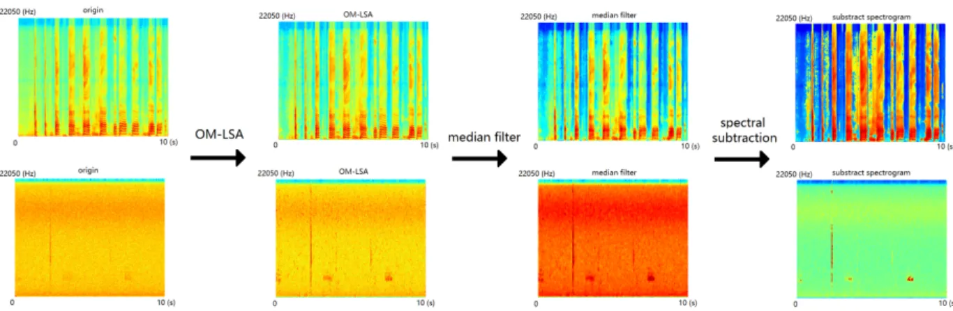
Fig. 3. First column: spectrogram of two audio recordings with different scene noise and level. Second column: spectrogram of OM-LSA algorithm denoised recordings. Third column: median filter enhanced spectrogram. Fourth column: spectral subtraction enhanced spectrogram

f(·). We use the binary crossentropy between the output and the ground truth as loss function and apply backpropogation on both the detector and the classifier to train the JDC model.

V. AUDIO DENOISING

The real audio recordings consist of not only the event sounds but also the background noise. The background noise may vary from scenes to scenes. Previous work suggests noise reduction is important in BAD [3]. For additive noise, the mixed sound can be decomposed by:

s(t) =x(t) +e(t) (3)

wheres(t),x(t)ande(t)are mixed sound, event sounds and scene noise, respectively. Without denoising, the features are extracted by applying the transformation T(·)ons(t), where T(·)is the short time Fourier transform (STFT):

S(t, f) =T(s(t)) (4)

wheretandf are indexes of the time axis and the frequency axis, respectively. Ideally, we want to eliminate the noisee(t)

from different scenes because the background noise usually carries little information and will worse the detecting of the sound events. We try to apply denoising algorithms on both the audio domain and the spectrogram. We assume the back-ground noise is stationary and only change slowly. First, we apply optimally-modified log-spectral amplitude (OM-SLA) [22] denoted asD1on each audio clip. Then median filter [23] and spectral subtraction [24] is applied on the spectrogram, denoted by D2 andD3, respectively. We denote the denoised spectrogram as:

e

S(t, f) =D3D2T(D1(s(t))) (5)

A. Optimally-modified log-spectral amplitude (OM-LSA)

Optimally-modified log-spectral amplitude (OM-LSA) is proposed by Cohen and applied to speech enhancement in 2001 [22]. The noise estimation is given by averaging past

spectral power values, using a smoothing parameter that is adjusted by the speech presence probability in subbands. OM-LSA can enhance the speech mixed with non-stationary noise, which is also applicable for enhancing the bird sounds. In Figure 3, the first column are spectrograms of two recordings under different noise. The second column shows their corre-sponding OM-LSA denoised spectrogram.

B. Median filter

Median filter is widely used to remove the salt-and-pepper noise in image processing [23]. Similarly, we can apply the median filter to the spectrogram because it can remove the salt-and-pepper noise on the spectrogram caused by random noise. On the other hand, the spectrogram of bird calls are continuous in both time and frequency domain so are not affected by median filter. After applying the median filter, the corresponding spectrograms are shown in the third column of Figure 3.

C. Spectral subtraction

Spectral subtraction is a simple and effective method for noise reduction [24]. A noise level is estimated from parts of the spectrogram for each frequency bin, for example, the median value of each frequency bin. Then Each frequency bin is subtracted by their noise level. The negative value obtained from subtraction is clipped to 0. The spectral subtraction enhanced spectrograms are shown in the fourth column of Figure 3.

VI. EXPERIMENTS

A. Data preparation

We use the bird detection challenge dataset [3] contain-ing Warblr [3] and Freefield1010 [16] as development data. Warblr dataset contains 10,000 ten-second (totally 44 hours) smartphone audio recordings from around UK. Freefield1010 contains 7,000 ten-second recordings from a diverse location and environment and is newly annotated for the BAD chal-lenge. We combine the two datasets and divide them to 10 folds, with 8 folds for training, 1 fold for validation and 1 fold for testing.

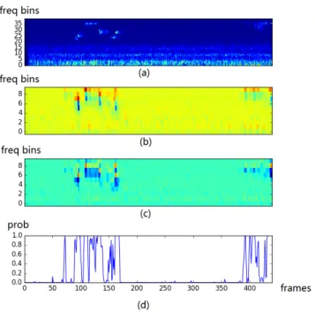
Fig. 4. (a) Mel spectrogram of an audio containing a bird. (b,c) Two feature maps after the last convolution operation before the global pooling. (d) Output of the detector.

We try both with denoising and without denoising for preprocessing data. For denoising, we apply OM-LSA on the audio recordings followed by median filter and spectral sub-traction on the spectrogram. We extracted 40 mel filter bank features with minimum frequency of 200 Hz and maximum frequency of 12000 Hz using librosa1_.

The configuration of the model is shown in Figure 1. We use Adam optimizer [25] with learning rate 0.001. The training takes around 2 minutes / epoch on a single TitanX GPU. The training takes around 50 epochs to converge. Code for JDC-CNN model is available online2_.

B. Results

Table 1 compares the results of different denoising strate-gies. We use no denoising with global max pooling and global average pooling as baseline. To speed up the training, in this sub-experiment we only one fold is used for training. From Table 1 we see in contrast to previous research [3], the classification area under curve (AUC) [26] was worse with denoising. On the other hand, JDC achieves comparable results with global max pooling and global mean pooling. Although JDC-CNN model does not outperform the baseline CNN model in AUC, Figure 4 shows JDC-CNN is able to detect when a bird calls from weakly labelled data by visualizing the detector.

As denoising will worse the classification result, we aban-don denoising in the following experiments. Table 2 compares how the training data size will affect the classification result. We experimented using 1 fold on 8 folds for training. Ob-viously, Table 2 shows the AUC increases with training data

1_{https://github.com/librosa/librosa} 2_{https://github.com/qiuqiangkong/bird detection} global max pooling (%) global mean pooling (%) JDC (%) no denoising 91.59+-0.46 91.48+-0.54 91.60+-0.45 OM-LSA 91.16+-0.20 91.32+-0.30 91.37+-0.20 OM-LSA +

me-dian filter + spec-tral subtraction

88.46+-0.42 89.32+-0.16 90.03+-0.32

TABLE II

AUCOF THE MODELS TRAINED ON DIFFERENT SIZE OF DATA

global max pooling (%) global mean pooling (%) JDC (%) train on 1 fold 91.59+-0.46 91.48+-0.54 91.60+-0.45 train on 8 folds 96.04+-0.22 95.88+-0.18 95.70+-0.18 TABLE III

AUCEVALUATED ON PRIVATE EVALUATION DATA

global max pooling (%) global mean pooling (%) JDC (%) private dataset 78.78 82.05 81.36 VII. CONCLUSION

In this paper, we propose to use joint detection and clas-sification convolutional neural network (JDC-CNN) on the weakly labelled bird audio dataset. JDC model consists of a detector modeled by CNN and a classifier modeled by VGG. The detector can attend to important events and ig-nore unimportant noise. The classifier outputs a probability indicating a frame contains a bird or not. By applying JDC-CNN, the weakly labelled data (WLD) can be converted to strongly labelled data (SLD). Furthermore, we show that de-noising methods including OM-LSA, median filter and spectral subtraction do not help the detection in contrast to previous research. In practice, the detector of JDC model sometimes has false alarms, that is the detector may attend to non-birds events wrongly, especially on the unseen data. In future, more work on JDC model will be explored.

VIII. ACKNOWLEDGEMENT

This research is supported by EPSRC grante EP/N014111/1 Making Sense of Sounds and scholarship from the China Scholarship Council (CSC). Thanks to the organizers for holding the bird detection challenge 2016.

REFERENCES

[1] Annamaria Mesaros, Toni Heittola, and Tuomas Virta-nen. Tut database for acoustic scene classification and sound event detection. In European Signal Processing Conference (EUSIPCO), pages 1128–1132. IEEE, 2016. [2] Dan Stowell, Dimitrios Giannoulis, Emmanouil Benetos, Mathieu Lagrange, and Mark D Plumbley. Detection and classification of acoustic scenes and events. IEEE Transactions on Multimedia, 17(10):1733–1746, 2015. [3] Dan Stowell, Mike Wood, Yannis Stylianou, and Herv´e

Glotin. Bird detection in audio: a survey and a challenge. In Machine Learning for Signal Processing (MLSP), Workshop on 2016 IEEE 26th International, pages 1–6. IEEE, 2016.

[4] Alex Krizhevsky, Ilya Sutskever, and Geoffrey E Hinton. Imagenet classification with deep convolutional neural networks. InAdvances in Neural Information Processing Systems, pages 1097–1105, 2012.

[5] Ossama Abdel-Hamid, Abdel-rahman Mohamed, Hui Jiang, Li Deng, Gerald Penn, and Dong Yu. Con-volutional neural networks for speech recognition.

IEEE/ACM Transactions on Audio, Speech, and Lan-guage Processing, 22(10):1533–1545, 2014.

[6] Anurag Kumar and Bhiksha Raj. Audio event detec-tion using weakly labeled data. In Proceedings of the 2016 ACM on Multimedia Conference, pages 1038–1047. ACM, 2016.

[7] Chiman Kwan, Gang Mei, X Zhao, Zhubing Ren, Roger Xu, Vincent Stanford, Cedric Rochet, Julian Aube, and KC Ho. Bird classification algorithms: Theory and experimental results. In Acoustics, Speech, and Signal Processing, 2004. Proceedings.(ICASSP’04)., volume 5, pages V–289. IEEE, 2004.

[8] Peter Janˇcoviˇc and M¨unevver K¨ok¨uer. Automatic de-tection and recognition of tonal bird sounds in noisy environments. EURASIP Journal on Advances in Signal Processing, 2011(1):982936, 2011.

[9] Ilyas Potamitis, Stavros Ntalampiras, Olaf Jahn, and Klaus Riede. Automatic bird sound detection in long real-field recordings: Applications and tools. Applied Acoustics, 80:1–9, 2014.

[10] Dan Stowell and Mark D Plumbley. Automatic large-scale classification of bird sounds is strongly improved by unsupervised feature learning. PeerJ, 2:e488, 2014. [11] Jos´e Francisco Ruiz-Mu˜noz, Mauricio Orozco-Alzate,

and Germ´an Castellanos-Dom´ınguez. Multiple instance learning-based birdsong classification using unsupervised recording segmentation. In IJCAI, pages 2632–2638, 2015.

[12] Forrest Briggs, Balaji Lakshminarayanan, Lawrence Neal, Xiaoli Z Fern, Raviv Raich, Sarah JK Hadley, Adam S Hadley, and Matthew G Betts. Acoustic classification of multiple simultaneous bird species: A multi-instance multi-label approach. The Journal of the Acoustical Society of America, 131(6):4640–4650, 2012. [13] Karen Simonyan and Andrew Zisserman. Very deep convolutional networks for large-scale image recognition.

arXiv preprint arXiv:1409.1556, 2014.

[14] Keunwoo Choi, George Fazekas, and Mark Sandler. Automatic tagging using deep convolutional neural net-works. arXiv preprint arXiv:1606.00298, 2016.

[15] Dan Stowell and Mark D Plumbley. Birdsong and c4dm: A survey of uk birdsong and machine recognition for music researchers.Centre for Digital Music, Queen Mary University of London, Tech. Rep. C4DM-TR-09-12, 2010. [16] Dan Stowell and Mark D Plumbley. An open dataset for research on audio field recording archives: freefield1010.

arXiv preprint arXiv:1309.5275, 2013.

[17] Herv´e Go¨eau, Herv´e Glotin, Willem-Pier Vellinga, Robert Planqu´e, and Alexis Joly. Lifeclef bird iden-tification task 2016: The arrival of deep learning. In

Working Notes of CLEF 2016-Conference and Labs of the Evaluation forum, ´Evora, Portugal, 5-8 September, 2016., pages 440–449, 2016.

[18] Ross Girshick, Jeff Donahue, Trevor Darrell, and Jitendra Malik. Rich feature hierarchies for accurate object detection and semantic segmentation. In Proceedings of the IEEE Conference on Computer Vision and Pattern Recognition, pages 580–587, 2014.

[19] Lindasalwa Muda, Mumtaj Begam, and Irraivan Elam-vazuthi. Voice recognition algorithms using mel frequency cepstral coefficient (mfcc) and dynamic time warping (dtw) techniques. arXiv preprint arXiv:1003.4083, 2010.

[20] Kaiming He, Xiangyu Zhang, Shaoqing Ren, and Jian Sun. Deep residual learning for image recognition. In

Proceedings of the IEEE Conference on Computer Vision and Pattern Recognition, pages 770–778, 2016.

[21] Qiuqiang Kong, Yong Xu, Wenwu Wang, and Mark Plumbley. A joint detection-classification model for audio tagging of weakly labelled data. arXiv preprint arXiv:1610.01797, 2016.

[22] Israel Cohen and Baruch Berdugo. Speech enhancement for non-stationary noise environments. Signal Process-ing, 81(11):2403–2418, 2001.

[23] Zhou Wang and David Zhang. Progressive switching median filter for the removal of impulse noise from highly corrupted images. IEEE Transactions on Circuits and Systems II: Analog and Digital Signal Processing, 46(1):78–80, 1999.

[24] Saeed V Vaseghi. Advanced digital signal processing and noise reduction. John Wiley & Sons, 2008. [25] Diederik Kingma and Jimmy Ba. Adam: A method for

stochastic optimization. arXiv preprint arXiv:1412.6980, 2014.

[26] James A Hanley and Barbara J McNeil. The meaning and use of the area under a receiver operating characteristic (roc) curve. Radiology, 143(1):29–36, 1982.