No. 533
Unconditional Quantile Regressions
Sergio Firpo
Nicole M. Fortin
Thomas Lemieux
TEXTO PARA DISCUSSÃO
Unconditional Quantile Regressions
∗
Sergio Firpo,
Pontif´ıcia Universidade Cat´olica - Rio
Nicole M. Fortin, and Thomas Lemieux
University of British Columbia
November 2006
Abstract
We propose a new regression method to estimate the impact of explanatory variables on quantiles of the unconditional distribution of an outcome variable. The proposed method consists of running a regression of the (recentered) influence function (RIF) of the unconditional quantile on the explanatory variables. The influence function is a widely used tool in robust estimation that can easily be computed for each quantile of interest. We show how standard partial effects, as well as policy effects, can be estimated using our regression approach. We propose three different regression estimators based on a standard OLS regression OLS), a Logit regression Logit), and a nonparametric Logit regression (RIF-NP). We also discuss how our approach can be generalized to other distributional statistics besides quantiles.
Keywords: Influence Functions, Unconditional Quantile, Quantile Regressions.
∗
We are indebted to Joe Altonji, Richard Blundell, David Card, Vinicius Carrasco, Marcelo Fer-nandes, Chuan Goh, Joel Horowitz, Shakeeb Khan, Roger Koenker, Thierry Magnac, Whitney Newey, Geert Ridder, Jean-Marc Robin, Hal White and seminar participants at Yale University, CAEN-UFC, CEDEPLAR-UFMG, PUC-Rio, IPEA-RJ and Econometrics in Rio 2006 for useful comments on this and earlier versions of the manuscript. We thank Kevin Hallock for kindly providing the birthweight data used in one of the applications, and SSHRC for financial support.
Contents
1 Introduction 1
2 Model Setup and Parameters of Interest 4
3 General Concepts 8
3.1 Definition and Properties of Recentered Influence Functions . . . 8
3.2 Impact of General Changes in the Distribution of X . . . 11
4 Application to Unconditional Quantiles 14 4.1 Recentered Influence Functions for Quantiles . . . 14
4.2 The UQPE and the structural form . . . 16
4.2.1 Case 1: Linear, additively separable model . . . 16
4.2.2 Case 2: Non-linear, additively separable model . . . 17
4.2.3 Case 3: Linear, separable, but heteroskedastic model . . . 18
4.2.4 General case . . . 19
5 Estimation 22 5.1 Recentered Influence Function and its Components . . . 23
5.2 Three estimation methods . . . 24
5.2.1 RIF-OLS Regression . . . 24
5.2.2 RIF-Logit Regression . . . 25
5.2.3 Nonparametric-RIF Regression (RIF-NP) . . . 26
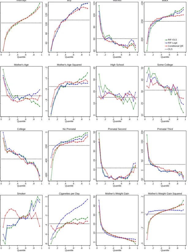
6 Empirical Applications 27 6.1 Determinants of Birthweight . . . 27
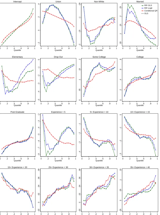
6.2 Unions and Wage Inequality . . . 28
6.2.1 Estimates of the Partial Effect of Unions . . . 28
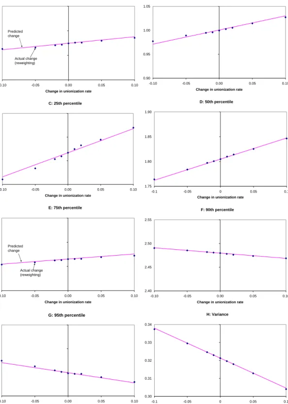
6.2.2 Estimates of the Policy Effect . . . 31
7 Conclusion 32
1
Introduction
One important reason for the popularity of OLS regressions in economics is that they pro-vide consistent estimates of the impact of an explanatory variable, X, on thepopulation unconditional mean of an outcome variable,Y. This important property stems from the fact that the conditional mean, E[Y|X], averages up to the unconditional mean, E[Y], due to the law of iterated expectations. As a result, a linear model for conditional means,
E[Y|X] =Xβ, implies that E[Y] =E[X]β, and OLS estimates ofβ also indicate what is the impact of X on the population average of Y. Many important applications of re-gression analysis crucially rely on this important property. For example, Oaxaca-Blinder decompositions of the earnings gap between blacks and whites or men and women, and policy intervention analyses (average treatment effect of education on earnings) all cru-cially depend on the fact that OLS estimates of β also provide an estimate of the effect of increasing education on the average earnings in a given population.
When the underlying question of economic and policy interest concerns other aspects of the distribution ofY, however, estimation methods that “go beyond the mean” have to be used. A convenient way of characterizing the distribution ofY is to compute its quan-tiles.1 This explains why conditional quantile regressions (Koenker and Bassett, 1978;
Koenker, 2005) have become increasingly popular. Unlike conditional means, however, conditional quantiles do not average up to their unconditional population counterparts. As a result, the estimates obtained by running a quantile regression cannot be used to estimate the impact ofX on the corresponding unconditional quantile. This implies that existing methods cannot be used to answer a question as simple as “what is the impact on median earnings of increasing everybody’s education by one year, holding everything else constant?”.
In this paper, we propose a new computationally simple regression method to estimate the impact of changes in the explanatory variables on the unconditional quantiles of the outcome variable. The method consists of running a regression of a transformation—the recentered influence function defined below—of the outcome variable on the explanatory variables. To distinguish our approach from commonly usedconditional quantile regres-sions, we call our regression method an unconditional quantile regression.2 Our approach
1Discretized versions of the distribution functions can be calculated using quantiles, as well many
inequality measurements such as, for instance, quantile ratios, inter-quantile ranges, concentration func-tions, and the Gini coefficient. This suggests modelling quantiles as a function of the covariates to see
how the whole distribution ofY responds to changes in the covariates.
2We obviously do not use the term “unconditional” to imply that we are not interested in the role
builds upon the concept of influence function (IF), a widely used tool in the robust esti-mation of statistical or econometric models. The IF represents, as its name suggests, the influence of an individual observation on a distributional statistic of interest. Influence functions of commonly used statistics are either well known or easy to derive. For exam-ple, the influence function of the mean µ=E[Y] is the demeaned value of the outcome variable, Y −µ.
Adding back the statistic to the influence function yields what we call theRecentered Influence Function (RIF). More generally, the RIF can be viewed as the contribution of an individual observation to a given distributional statistic. It is easy to compute the RIF for quantiles or most distributional statistics. For a quantile, the influence function IF (Y, qτ) is known to be equal to (τ −1I{Y ≤qτ})/fY (qτ), where 1I{·} is an indicator
function, fY (·) is the density of the marginal distribution of Y, and qτ = Qτ[Y] is the
population τ-quantile of the unconditional distribution of Y.3 As a result, RIF (Y;qτ) is
simply equal to qτ + IF (Y, qτ).
We call the conditional expectation of the RIF (Y;ν) modelled as a function of the explanatory variables,E[RIF (Y;ν)|X] = mν(X), the RIF-regression model. In the case
of the mean, since the RIF is simply the value of the outcome variable, Y, a regression of RIF (Y;µ) on X is the same as the standard regression of Y on X. This explains why, in our framework, OLS estimates are valid estimates of the effect of X on the unconditional mean of Y. More importantly, we show that this property extends to any other distributional statistic. For the τ-quantile, we show the conditions under which a regression of RIF (Y;qτ) onX can be used to consistently estimate the effect of X on the
unconditional τ-quantile of Y. In the case of quantiles, we call the RIF-regression model,
E[RIF (Y;qτ)|X] = mτ(X), an unconditional quantile regression. We define, in Section
4, the exact population parameters that we estimate using this regression. The first parameter is the partial (or marginal) effect of shifting the distribution of a covariate on the unconditional quantile. The second parameter is the effect of a more general change in the distribution of covariates that corresponds to Stock’s (1989) “policy effect”.
Importantly, we show that these two parameters are nonparametrically identified under sufficient assumptions that guarantee that the conditional distribution of the
out-outcome variableY, i.e. the distribution obtained by integrating the conditional distribution ofY given
X over the distribution ofX. Using “marginal” instead of “unconditional” would be confusing, however,
since we also use the word “marginal” to refer to the impact of small changes in covariates (marginal effects).
3We define the unconditional quantile operator as Q
τ[·]≡infqPr [· ≤q] ≥τ. Similarly, the
come variable Y does not change in response to a change in the distribution of covari-ates. We view our approach as an important contribution to the literature concerned with the identification of quantile functions. However, unlike contributions to that area such as Chesher (2003), Florens, Heckman, Meghir, and Vytlacil (2003), and Imbens and Newey (2005), which consider the identification of structural functions defined from conditional quantile restrictions, our approach is concerned solely with parameters that capture changes in the unconditional quantiles.
We also view our method as a very important complement to conditional quantile regressions. Of course, in some settings quantile regressions are the appropriate method to use.4 For instance, quantile regressions are a useful descriptive tool that provide a
parsimonious representation of the conditional quantiles. Unlike standard OLS regression estimates, however, quantile regression estimates cannot be used to assess the more general economic or policy impact of a change ofX on the corresponding quantile of the unconditional distribution of Y. While OLS estimates can be used as estimates of the effect of X on either the conditional or the unconditional mean, one has to be much more careful in deciding what is the ultimate object of interest in the case of quantiles.
For instance, consider one example of quantile regressions studied by Chamberlain (1994): the effect of union status on log wages. An OLS estimate of the effect of union on log wages of 0.2, for example, means that a decline of 1 percent in the rate of unionization would lower average wages by 0.2 percent. But if the estimated effect of unions (using quantile regressions) on the conditional 90th quantile is 0.1, this does not mean that a decline of 1 percent in the rate of unionization would lower the unconditional 90th quantile by 0.1 percent. In fact, we show in an empirical application in Section 6 that unions have a positive effect on the conditional 90th quantile, but a negative effect on
the unconditional 90th quantile. If we are interested in the overall effect of unions
on wage inequality, our unconditional quantile regressions should be used to obtain the effect of unions at different quantiles of the unconditional distribution. Using conditional quantile regressions to estimate the overall effect of unions on wage inequality would yield a misleading answer in this particular case.
The structure of the paper is as follows. In the next section, we present the basic model and define two key objects of interest in the estimation: the “unconditional quan-tile partial effect” (UQPE) and the “policy effect”. In Section 3, we present the general properties of recentered influence functions. We formally show how the recentered
in-4See, for example, Buchinsky (1994) and Chamberlain (1994) for applications of conditional quantile
fluence function can be used to compute what happens to a distributional statistic ν
when the distribution of the outcome variable Y changes in response to a change in the distribution of the covariates X. In Section 4, we focus on quantiles and show how un-conditional quantile regressions can be used to estimate either the policy effect or the UQPE. Considering an explicit structural model between Y and X, we discuss the links between the structural parameters and the UQPE for some specific examples and for the general case. Estimation issues are addressed in Section 5. Section 6 presents two applications of our method: the determinants of the distribution of infants’ birthweight (as in Koenker and Hallock, 2001) and the impact of unions on the distribution of log wages. We conclude in Section 7.
2
Model Setup and Parameters of Interest
Before presenting the estimation method, it is important to clarify exactly what the unconditional quantile regressions seek to estimate. Assume that we observe Y in the presence of covariates X, so that Y andX have a joint distribution,FY,X(·,·) :R× X →
[0,1], and X ⊂ Rk is the support of X. Assume that the dependent variable Y is a
function of observables X and unobservables ε, according to the following model:
Y =h(X, ε),
where h(·,·) is an unknown mapping. Note that using a flexible functionh(·,·) is impor-tant for allowing for rich distributional effect of X on Y.5
We are primarily interested in estimating two population parameters, the uncondi-tional quantile partial effect and the policy effect, using uncondiuncondi-tional quantile regres-sions. We now formally define these two parameters.
Unconditional Quantile Partial Effect (UQPE)
By analogy with a standard regression coefficient, our first object of interest is the effect on an unconditional quantile of a small increase t in the explanatory variable
5A number of recent studies also use general nonseparable models to investigate a number of related
issues. See, for example, Chesher (2003), Florens, Heckman, Meghir, and Vytlacil (2003), and Imbens and Newey (2005).
X. This effect of a small change in a continuous variable X on the τth quantile of the unconditional distribution of Y, is defined as:
α(τ) = lim
t↓0
Qτ[h(X +t, ε)]−Qτ[Y]
t
where Qτ[Y] is theτth quantile of the unconditional distribution of the random variable
Y.6
We call this parameter, α(τ), the unconditional quantile partial effect (UQPE), by analogy with Wooldridge (2004) unconditional average partial effect (UAPE), which is defined as E[∂E[Y|X]/∂x]. The link between α(τ) and Wooldridge’s UAPE can be established using a result of Section 3 where we show that for any statistic ν de-fined as a functional of the unconditional distribution of Y, α(ν) is exactly equal to
E[∂E[RIF(Y, ν)|X]/∂x]. In the case of the mean, since RIF(Y, µ) =Y, α(µ) is indeed equal to Wooldridge’s UAPE = limt↓0 E[h(X +t, ε)]−E[Y]
/t. In the case of quantiles, derived in Section 4, our parameter of interestα(τ) corresponds toE∂ERIF(Y, qτ)|X
/∂x and is named UQPE.
Similarly, by analogy with Wooldridge’s (2004) conditional average partial effect (CAPE) defined as ∂E[Y|X]/∂x, we can think of conditional quantile regressions as a method for estimating the partial effects of the conditional quantiles of Y given a par-ticular value X. We refer to this type of quantile partial effects as “conditional quantile partial effects” (CQPE) and define them as ∂Qτ[Y|X]/∂x= limt↓0 Qτ[h(X +t, ε)|X]
−Qτ[Y|X]
/t in Section 4.
Note that while the UAPE equals the average CAPE, the same relationship does not hold between the UQPE and the CQPE. We will indeed show in Section 4 that the UQPE is equal to a complicated weighted average of the CQPE over the whole range of conditional quantiles (i.e. for τ going from 0 to 1).
Policy Effect
We are also interested in estimating the impact of a more general change in X on the τth quantile ofY. Consider the “intervention” or “policy change” proposed by Stock
6To simplify the exposition we are treating X as univariate. However, this is easily generalized to
the multivariate case by defining for eachj = 1, ..., k,
αj(τ) = lim
tj↓0
Qτ[h([Xj+tj;X−j], ε)]−Qτ[Y]
tj
(1989) and Imbens and Newey (2005), where X is replaced by the function `(X), ` :
X → X.7 For example, if X represents years of schooling, a compulsory high school completion program aimed at making sure everyone completes grade twelve would be captured by the policy function`(·), where`(X) = 12 ifx≤12, and `(X) =xotherwise. We define δ`(τ) as the effect of the policy on the τth quantile of Y, where
δ`(τ) =Qτ[h(`(X), ε)]−Qτ[Y].
In the case of the mean we have
δ`(µ) =E[h(`(X), ε)]−E[Y] =E[E[h(`(X), ε)−h(X, ε)|X]]
which corresponds to the mean of the policy effect proposed by Stock (1989).
The main contribution of the paper is to show that a regression framework where the outcome variable Y is replaced by RIF(Y, qτ) can be used to estimate the unconditional
partial effect α(τ) and the policy effect δ`(τ) for quantiles. We show this formally in
Section 3, after having introduced some general concepts. Since these general concepts hold for any functional of the distribution of interest, the proposed regression framework extends to other distributional statistics such as the variance or the Gini coefficient.
Before introducing these general concepts, however, a few remarks are in order. First, both the UQPE and the policy effect involve manipulations of the explanatory variables that can be modelled as changes in the distribution of X, FX(x).
Un-der the “policy change”, `(X), the resulting counterfactual distribution is given by
GX(x) = FX(`−1(x)).8 Representing manipulations of X in terms of the
counterfac-tual distribution, GX(x), makes it easier to derive the impact of the manipulation on
FY (y), the unconditional distribution of the outcome variable Y. By definition, the
unconditional (marginal) distribution function of Y can be written as
FY (y) =
Z
FY|X(y|X =x)·dFX(x). (1)
Under the assumption that the conditional distributionFY|X(·) is unaffected by
ma-nipulations of the distribution of X, a counterfactual distribution of Y, GY, can be
7Here, we focus first on a policy function that is independent of the error term ε. That is, where
non-compliance, for example, would be random.
8If`(·) is not globally invertible, we may actually break down the support ofX in regions where the
function is invertible. This allowsGX(x) =FX `−1(x)
obtained by replacing FX(x) withGX(x):
GY (y)≡
Z
FY|X(y|X =x)·dGX(x). (2)
Although the construction of this counterfactual distribution looks purely mechanical, important economic conditions are imbedded in the assumption thatFY|X(·) is unaffected
by manipulations of X. Because Y = h(X, ε), a sufficient condition for FY|X(·) to be
unaffected by manipulations ofX is thatεis independent ofX. For the sake of simplicity, we implicitly maintain this assumption throughout the paper, although it may be too strong in specific cases.9 Sinceh(X, ε) can be very flexible, independence ofεandX still allows for unobservables to have rich distributional impacts.
A second remark is that, as in the case of a standard regression model for conditional means, there is no particular reasons to expect RIF regression models to be linear in X. In fact, in the case of quantiles we show in Section 4 that even for the most basic linear model, h(X, ε) = Xβ+ε, the RIF regression is not linear. Fortunately, the non-linear nature of the RIF regression is closely related to the problem of estimating a regression model for a dichotomous dependent variable. Widely available estimation procedures (Probit or logit) can thus used to deal the special nature of the RIF for quantiles. In the empirical Section 6 we show that, in practice, different regression methods yield very similar estimates of the UQPE. This finding is not surprising in light of the “common empirical wisdom” that Probits, logits, and linear probability models all yield very similar estimates of average marginal effects in a wide variety of cases.
A final remark is that while our regression method yields exact estimates of the UQPE, it only yields a first order approximation of the policy effect δ`(τ). In other words, how
accurate our estimates of δ`(τ) are in the case of larger changes in the distribution ofX
turns out to be an empirical question. We show in Section 6 that, in the case of unions and wage inequality, our method yields very accurate results even in case of economically large changes in the rate of unionization.
9The independence assumption can easily be relaxed. For instance, if X = (X
1, X2) and onlyX1
is being manipulated, it is sufficient to assume that ε is independent of X1 conditional on X2. This
conditional independence assumption is similar to the “ignorability” or “unconfoundedness” assumption
commonly used in the program evaluation literature. Independence between εand of X could also be
obtained by conditioning on a control function constructed using instrumental variables, as in Chesher (2003), Florens et al., (2003), and Imbens and Newey (2005).
3
General Concepts
In this section we first review the concept of the influence function, which arises in the von Mises (1947) approximation and is largely used in the robust statistics literature. We then introduce the recentered influence function, which is central to the derivation of unconditional quantile regressions. Finally, we apply the von Mises approximation, defined for a general alternative or counterfactual distribution, to the case of where this counterfactual distribution arises from changes in the covariates. The derivations are developed for general functionals of the distribution; they will be applied to quantiles (and the mean) in the next section.
3.1
Definition and Properties of Recentered Influence
Func-tions
We begin by recalling the theoretical foundation of the definition of the influence function, following Hampel et al. (1986). For notational simplicity, in this subsection we drop the subscript Y on FY and GY. Hampel (1968, 1974) introduced the influence function as
a measure to study the infinitesimal behavior of real-valued functionals ν(F), where
ν : Fν → R, and where Fν is a class of distribution functions such that F ∈ Fν if
|ν(F)| < +∞. In our setting, F is the CDF of the outcome variable Y, while ν(F) is a distributional statistic such as a quantile. Following Huber (1977), we say that ν(·) is Gˆateaux differentiable at F if there exists a real kernel functiona(·) such that for all G
in Fν: lim t↓0 ν(Ft,G)−ν(F) t = ∂ν(Ft,G) ∂t |t=0 = Z a(y)·dG(y), (3)
where 0 ≤t≤1, and where the mixing distributionFt,G
Ft,G≡(1−t)·F +t·G=t·(G−F) +F (4)
is the probability distribution that is t away from F in the direction of the probability distribution G.
The expression on the left hand side of equation (3) is the directional derivative of ν
(3) by d(G−F) (y), we get: lim t↓0 ν((1−t)·F +t·G)−ν(F) t = ∂ν(Ft,G) ∂t |t=0 = Z a(y)·d(G−F) (y) (5)
since R a(y)·dF(y) = 0, which follows by considering the case where G=F.
The concept of influence function arises from the special case whereG is replaced by ∆y , the probability measure that put mass 1 at the value y in the mixture Ft,G. This
yields Ft,∆y, the distribution that contains a blip or a contaminant at the point y,
Ft,∆y ≡(1−t)·F +t·∆y.
The influence function of the functional ν at F for a given point y is defined as
IF(y;ν, F) ≡ lim t↓0 ν(Ft,∆y)−ν(F) t = ∂ν Ft,∆y ∂t |t=0 = Z a(y)·d∆y(y) = a(y). (6)
By a normalization argument, IF(y;ν, F), the influence function of ν evaluated at y
and at the starting distribution F will be written as IF(y;ν). Using the definition of the influence function, the functional ν(Ft,G) itself can be represented as a von Mises linear
approximation (VOM):10
ν(Ft,G) =ν(F) +t·
Z
IF(y;ν)·d(G−F) (y) +r(t;ν;G, F) (7)
where r(t;ν;G, F) is a remainder term that converges to zero as t goes to zero at the general rateo(t). Depending on the functionalν considered, the remainder may converge faster or even be identical to zero. For example, for the mean µ, r(t;µ;G, F) = 0, while for the quantile qτ, r(t;qτ;G, F) = o(t). Also, if F = G, then r(t;ν;F, F) = 0 for any
t or ν. More generally, the further apart the distributions F and G are, the larger the remainder term should be.11
Now consider the leading term of equation (7) as an approximation forν(G), that is,
10This expansion can be seen as a Taylor series approximation of the real function A(t) = ν(F
t,G)
aroundt= 0 :A(t) =A(0) +A0(0)·t+Rem
1. But sinceA(0) =ν(G), andA0(0) =Ra1(y)d(G−F) (y),
where a1(y) is the influence function, we get the VOM approximation.
11If we fixνandt(for example, by making it equal to 1) and allowFandGto be empirical distributions
b
for t= 1:
ν(G)≈ν(F) +
Z
IF(y;ν)·dG(y). (8)
By analogy with the influence function, for the particular case G= ∆y, we call this first
order approximation term the Recentered Influence Function (RIF) RIF(y;ν, F) =ν(F) +
Z
IF(y;ν)·d∆y(y) =ν(F) + IF(y;ν). (9)
Again, by a normalization argument, we write RIF(y;ν, F) as RIF(y;ν). The recentered influence function RIF(y;ν) has several interesting properties:
Property 1 [Mean and Variance of the Recentered Influence Function]:
i) the RIF(y;ν) integrates up to the functional of interest ν(F)
Z
RIF(y;ν)·dF(y) =
Z
(ν(F) + IF(y;ν))·dF(y) =ν(F). (10)
ii) the variance of RIF(y;ν) under F equals the asymptotic variance of the functional
ν(F) Z
(RIF(y;ν)−ν(F))2·dF(y) =
Z
(IF(y;ν))2·dF(y) =AV (ν, F) (11)
where AV (ν, F) is the asymptotic variance of functional ν under the probability distri-bution F.
Property 2 [Recentered Influence Function and the Directional Derivative]:
i) the derivative of the functional ν(Ft,G)in the direction of the distributionGis obtained by integrating up the recentered influence function at F over the distributional differences between G and F
∂ν(Ft,G)
∂t |t=0= Z
RIF(y;ν)·d(G−F) (y). (12)
ii) the Von Mises approximation (7) can be written in terms of the RIF(y;ν) as
ν(Ft,G) =ν(F) +t·
Z
RIF(y;ν)·d(G−F) (y) +r(t;ν;G, F) (13)
where the remainder term is
r(t;ν;G, F) =
Z
(RIF(y;ν, Ft,G)−RIF(y;ν))·dFt,G(y).
proof is provided here. In fact, Property 1 follows from the usual definition of the influence function, while Property 2 combines equations (5), (6) and (9), and follows from the fact that densities integrate to one. Finally, note that properties 1 ii) and 2 i) and ii) are also shared by the influence function.
3.2
Impact of General Changes in the Distribution of
X
We now show that the recentered influence function provides a convenient way of assessing the impact of changes in the covariates on the distributional statistic ν without having to compute the corresponding counterfactual distribution of Y which is, in general, a difficult estimation problem. We first consider general changes in the distribution of covariates, from FX(x) to the counterfactual distribution GX (x). We then consider
the special case of a marginal change from X to X +t, and of the policy change `(X) introduced in Section 2.
In the presence of covariatesX, we can use the law of iterated expectations to express
ν in terms of the conditional expectation of RIF(y;ν) givenX,
Property 3 [The functional ν(FY) and the RIF-regression]:
The conditional expectation ofRIF(y;ν)givenX integrates up to the functional of interest
ν(FY) ν(FY) = Z RIF(y;ν)·dFY(y) = Z E[RIF(Y;ν)|X =x]·dFX(x) (14)
where we have substituted equation (1) into equation (10), and used the fact that
E[RIF(Y; ν)|X =x] = RyRIF(y;ν)·dFY|X(y|X =x). Property 3 is central to our
ap-proach. It provides a simple way of writing any functionalν of the distribution as an ex-pectation and, furthermore, to writeνas the mean of the RIF-regressionE[RIF(Y;ν)|X]. Comparing equation (1) and property 3 illustrates how our approach greatly simplifies the modelling of the effect of covariates on distribution statistics. In equation (1), the whole conditional distribution, FY|X(y|X =x), has to be integrated over the distribution ofX
to get the unconditional distribution ofY,FY.12 When we are only interested in a specific
distribution statistic ν(FY), however, we simply need to integrate overE[RIF(Y;ν)|X],
which is easily estimated using regression methods.
12This is essentially what Machado and Mata (2005) suggest to do, since they propose estimating the
whole conditional distribution by running (conditional) quantile regressions for each and every possible
quantile. See also Albrecht, Bj¨orklund and Vroman (2003), Gardeazabal and Ugidos (2005), and Melly
(2005) for related attempts at performing Oaxaca-Blinder type decompositions of unconditional quantiles using conditional quantile regressions.
Property 3 also suggests that the counterfactual values ofν can be obtained by inte-grating over a counterfactual distribution of X instead ofFX(x). The following theorem
indeed states that the effect (on the functionalν) of a small change in the distribution of covariates from FX in the direction of GX is given by integrating up the RIF-regression
function with respect to the change in distribution of the covariates,d(GX −FX).
Theorem 1 [Marginal Effect of a Change in the Distribution of X]:
πG(ν) ≡ ∂ν(FY,t,G) ∂t |t=0 = limt↓0 ν(FY,t,GY)−ν(FY) t = Z RIF(y;ν)·d(GY −FY) (y) = Z E[RIF(Y;ν)|X =x]·d(GX −FX) (x)
The proof, provided in the appendix, is based on applying the law of iterated expectations to equation (12).
Consider the implications of Theorem 1 for the policy effect and the unconditional partial effect introduced in Section 2. Given that πG(ν) captures the marginal effect of
moving the distribution of X from FX to GX, it can be used as the leading term of an
approximation, just like equation (12) is the leading term of the von Mises approximation (equation (13)). Our first corollary shows how this fact can be used to approximate the policy effect δ`(ν).
Corollary 1 [Policy Effect]: If a policy change from X to `(X) can be described
as a change in the distribution of covariates, that is, `(X) ∼ GX, where GX (x) =
FX(`−1(x)), then δ`(ν), the policy effect on the functional ν, consists of the marginal effect of the policy, π`(ν), and a remainder term r(ν, GY, FY):
δ`(ν) =ν(GY)−ν(FY) =π`(ν) +r(ν;GY, FY) where π`(ν) = Z E[RIF(Y;ν)|X =x]· dFX(`−1(x))−dFX(x) , and r(ν;GY, FY) = Z (E[RIF(Y;ν, GY)|X =x]−E[RIF(Y;ν)|X =x])·dFX(`−1(x)))
No proof for Corollary 1 is provided since, given Theorem 1, it is a immediate consequence of Property 2 ii) making t= 1. Note that the approximation errorr(ν;GY, FY) depends
on how different the means of RIF(Y;ν) and RIF(Y;ν, GY) are under the new distribution
of covariates GX.13
The next case is the unconditional partial effect ofXonν, defined asα(ν) in Section 2. The implicit assumption here is that X is a continuous covariate that is being increased from X to X+t. We consider the case where X is discrete in the third corollary below.
Corollary 2 [Unconditional Partial Effect: Continuous Covariate]: Consider
increasing a continuous covariate X by t, fromX to X +t. This change results in the counterfactual distribution FY,t∗ (y) =
R
FY|X(y|x)·dFX(x−t). The effect of X on the distributional statistic ν, α(ν), is α(ν) ≡ lim t↓0 ν F∗ Y,t −ν(FY) t = Z dE[RIF(Y;ν)|X =x] dx ·dF(x).
The proof is provided in the appendix. The corollary simply states that the effect (on
ν) of a small change in covariate X is equal to the average derivative of the recentered influence function with respect to the covariate.14
Finally, we consider the case where X is a dummy variable. The manipulation we have in mind here consists of increasing the probability that X is equal to one by a small amount t
Corollary 3 [Unconditional Partial Effect: Dummy Covariate]: Consider the
case where X is a discrete (dummy) variable, X ∈ {0,1}. Define PX ≡ Pr[X = 1]. Consider an increase from PX to PX +t. This results in the counterfactual distribution
FY,t∗ (y) =FY|X(y|1)·(PX +t) +FY|X(y|0)·(1−PX −t). The effect of a small increase in the probability that X = 1 is given by
αD(ν) ≡ lim t↓0 ν F∗ Y,t −ν(FY) t = E[RIF(Y;ν, F)|X = 1]−E[RIF(Y;ν, F)|X = 0]
The proof is, once again, provided in the appendix.
13We discuss this issue in more detail in Section 6.
4
Application to Unconditional Quantiles
In this section, we apply the results of Section 3 to the case of quantiles. We first derive the functional form of the RIF for quantiles and show that the UQPE can be obtained using RIF-regressions without reference to a specific functional form for the structural model Y =h(X, ε). We then look at a few specific structural models that help interpret the RIF-regressions in terms the underlying structural model and provide some guidance on the functional form of the RIF-regressions. We finally consider the case of a general model Y =h(X, ε) and derive the link between the UQPE and the underlying structural form. We also show the precise link between the UQPE and the CQPE, which is closely connected to the structural form.
4.1
Recentered Influence Functions for Quantiles
As a benchmark, first consider the case of the mean, ν(F) =µ. Applying the definition of the influence function (equation (6)) to µ = R y·dF(y), we get IF(y;µ) = y−µ, and RIF(y;µ) = µ+ IF(y;µ) = y. When the VOM linear approximation of equation (13) is applied to the mean, the remainder r(t;µ;G, F) equals zero since RIF(y;µ) = RIF(y;µ, Ft,G) =y.
Turning to our application of interest, consider theτth quantile,ν(F) =q
τ. Applying
the definition of the influence function to qτ, it follows that
IF(y;qτ) =
τ −1I{y≤qτ}
fY (qτ)
.
The influence function is simply a dichotomous variable that takes on the value −(1−τ)
/fY (qτ) when Y is below the quantileqτ, andτ /fY (qτ) whenY is above the quantileqτ.
The recentered influence function can thus be written as
RIF(y;qτ) =qτ+ IF(y;qτ) = qτ + τ −1I{y≤qτ} fY (qτ) = 1I{y > qτ} fY (qτ) +qτ − 1−τ fY (qτ) = c1,τ ·1I{y > qτ}+c2,τ.
where c1,τ = 1/fY (qτ) and c2,τ =qτ−c1,τ·(1−τ). Note that equation (10) implies that
the mean of the recentered influence function is the quantileqτ itself, and equation (11)
implies that its variance is τ ·(1−τ)/f2
The main results in Section 3 all involve the conditional expectation of the RIF. In the case of quantiles, we have
E[RIF(Y;qτ)|X =x] = c1,τ ·E[1I{Y > qτ} |X =x] +c2,τ
= c1,τ ·Pr [Y > qτ|X =x] +c2,τ. (15)
Since the conditional expectation E[RIF(Y;ν)|X =x] is a linear function of Pr[Y > qτ |X = x], it can be estimated using Probit or Logit regressions, or a simple OLS
regression (linear probability model). The parameters c1,τ and c2,τ can be estimated
using the sample estimate of qτ and a kernel density estimate of fY (qτ).15 Note that for
other functionalsνbesides quantiles, the estimation of the modelE[RIF(Y;ν)|X =x] =
mν(X) may be more appropriately pursued by nonparametric methods. These estimation
issues are discussed in detail in the next section.
The estimated model can then be used to compute either the policy effect or the UQPE defined in Corollaries 1 to 3. From Corollary 2, we have that the unconditional partial effect with continuous regressors , α(τ), is
U QP E(τ) = α(τ) = Z dE[RIF(Y;qτ)|X =x] dx ·dFX(x) (16) = 1 fY (qτ) · Z dPr [Y > qτ|X =x] dx ·dFX(x) (17) = c1,τ · Z dPr [Y > qτ|X =x] dx ·dFX(x) (18)
The integral in the above equation is the average “marginal” effect of the covariates in a probability response model (see, e.g., Wooldridge (2002)).16
Interestingly, the UQPE for a dummy regressor is also closely linked to a standard marginal effect in a probability response model. In this case, it follows from Corollary 3 that U QP E(τ) = αD(τ) = 1 fY (qτ) ·(Pr [Y > qτ|X = 1]−Pr [Y > qτ|X = 0]) = c1,τ ·(Pr [Y > qτ|X = 1]−Pr [Y > qτ|X = 0]).
15See Section 5 for more detail.
16Note that the marginal effect is often computed as the effect ofXon the probability for the “average
observation”,dPr [Y ≥qτ|X=x]/dx. This is how STATA, for example, computes marginal effects. The
At first glance, the fact that the UQPE is closely linked to standard marginal effects in a probability response model is a bit surprising. Consider a particular value y0 of Y
that corresponds to the τth quantile of the distribution ofY, qτ. Except for the scaling
factor 1/fY (qτ), our results mean that a small increase inX has the same impact on the
probability that Y is above y0, than on the τth unconditional quantile of Y. In other
words, we can transform a probability impact into an unconditional quantile impact by simply multiplying the probability impact by 1/fY (qτ). Roughly speaking, the reason
why the scaling factor 1/fY (qτ) provides the right transformation is that the function
that transforms probabilities into unconditional quantiles is the inverse of the cumulative distribution function, FY−1(y), and the slope of FY−1(y) is the inverse of the density, 1/fY (qτ). In essence, the proposed approach enables us to turn a difficult estimation
problem (the effect ofX on unconditional quantiles ofY) into an easy estimation problem (the effect of X on the probability of being above a certain value of Y).
4.2
The UQPE and the structural form
In Section 2, we first defined the UQPE and the policy effect in terms of the structural form Y = h(X, ε), where h(·) is now assumed to be strictly monotonic in ε. We now re-introduce the structural form to show how it is linked to the RIF-regression model,
E[RIF(Y;qτ)|X =x] = mτ(X). This is useful for interpreting the parameters of the
RIF-regression model, and for suggesting possible functional forms for the regression. We explore these issues using three specific examples of the structural form, and then discuss the link between the UQPE and the structural form in the most general case where h(·) is completely unrestricted (aside from the monotonicity in ε). Even in this general case, we show that the UQPE can be written as a weighted average of the CQPE, which is closely connected to the structural form, for different quantiles and values of X.
4.2.1 Case 1: Linear, additively separable model
We start with the simplest linear modelY =h(X, ε) =X|β+ε. As discussed in Section
2, we limit ourselves to the case where X and ε are independent. The linear form of the model implies that a small change t in a covariate Xj simply shifts the location of the
distribution of Y by βj ·t, but leaves all other features of the distribution unchanged.
As a result, the UQPE for any quantile is equal to βj. While β could be estimated using
a standard OLS regression in this simple case, it is nonetheless useful to see how it could also be estimated using our proposed approach.
For the sake of simplicity, assume that ε follows a distribution Fε. The resulting
probability response model is17
Pr [Y > qτ|X =x] = Pr [ε > qτ−x|β] = 1−Fε(qτ−x|β).
Thus if ε was normally distributed, the probability response model would be a standard Probit model. Taking derivatives with respect to Xj yields
dPr [Y > qτ|X =x]
dXj
=βj·fε(qτ−x|β),
wherefε is the density ofε, and the marginal effects are obtained by integrating over the
distribution of X Z
dPr [Y > qτ|X =x]
dxj
·dFX(x) =βj ·E[fε(qτ−X|β)],
where the expectation on the right hand side is taken over the distribution of X and the expression inside the expectation operator is simply the conditional density of Y
evaluated at Y =qτ: fε(qτ −x|β) =fY|X(qτ|X =x). It follows that
Z
dPr [Y > qτ|X =x]
dxj
·dFX (x) = βj·E[fY|X(qτ|X =x)] =βj·fY(qτ),
and by substituting back in equation (17), the UQPE is indeed found to equal βj
U QP Ej(τ) =
1
f(qτ)
·βj ·fY(qτ) =βj.
4.2.2 Case 2: Non-linear, additively separable model
A simple extension of the linear model is the index model h(X, ε) = ˜h(X|β+ε), where
˜
h is differentiable and strictly monotonic. When ˜h is non-linear, a small change t in a covariate Xj does not correspond to a simple location shift of the distribution ofY, and
the UQPE is no longer equal to β. One nice feature of the model, however, is that it yields the same probability response model as in Case 1. We have
Pr [Y > qτ|X =x] = Pr h ε >˜h−1(qτ)−x|β i = 1−Fε ˜ h−1(qτ)−x|β . 17Since q
The average marginal effects are now Z dPr [Y > qτ|X =x] dxj ·dFX(x) =βj ·E h fε ˜ h−1(qτ)−X|β i ,
and the UQPE is
U QP Ej(τ) =βj· Ehfε ˜ h−1(q τ)−X|β i fY(qτ) =βj·˜h 0˜ h−1(qτ) ,
where the last equality follows from the fact that
fY (qτ) = dPr [Y ≤qτ] dqτ = dE[Pr [Y ≤qτ|X]] dqτ = dEhFε ˜ h−1(q τ)−X|β i dqτ =E fε ˜ h−1(q τ)−X|β ˜ h0h˜−1(q τ) . Since ˜h0˜h−1(q τ)
depends on qτ, it follows that the UQPE is proportional, but not
equal, to the underlying structural parameter β. Also, the UQPE does not depend on the distribution of ε. The intuition for this result is simple. From Case 1, we know that the effect of Xj on the τth quantile of the index (X|β +ε) is βj. But since Y
and (X|β+ε) are linked by a rank preserving transformation ˜h(·), the effect on theτth
quantile of Y corresponds to the effect on the τth quantile of the index (X|β+ε) times the slope of the transformation function evaluated at this point, ˜h0
˜
h−1(qτ)
.18
4.2.3 Case 3: Linear, separable, but heteroskedastic model
A more standard model used in economics is the linear, but heteroskedastic model
h(X, ε) =X|β+σ(X)·ε, where X and εare still independent, but whereV ar(Y|X) =
σ2(X).19 The special case where σ(X) = X|ψ has the interesting implication that the conventional conditional quantile regression functions are also linear inX, an assumption
18Note that the UQPE could also be obtained by estimating the index model using a flexible form
for ˜h(·) (see, for example, Fortin and Lemieux (1998)). Estimating a flexible form for ˜h(·) and taking
derivatives is more difficult, however, than just computing average marginal effects and dividing them
by the density f(qτ). More importantly, since the index model is somewhat restrictive, it is important
to use a more general approach that is robust to the specifics of the structural formh(X, ε).
typically used in practice. To see this, consider the τth conditional quantile of Y,
Qτ[Y|X =x] =Qτ[X|β+ (X|ψ)·ε|X =x] = x|(β+Qτ[ε]·ψ),
where Qτ[ε] is the τth quantile of ε.20 This particular specification of h(X, ε) can also
be related to the quantile structural function (QSF) of Imbens and Newey (2005). In the case where ε is univariate, Imbens and Newey define the QSF as Qτ[Y|X =x] =
h(x, Qτ[ε]), which simply corresponds to x|(β +Qτ[ε]·ψ), the special linear case
con-sidered here.
The implied probability response model is the heteroskedastic model
Pr [Y > qτ|X =x] = Pr ε > −(x | β−qτ) x|ψ = 1−Fε qτ−x|β x|ψ . (19)
As is well known (e.g. Wooldridge, 2002), introducing heteroskedasticity greatly com-plicates the interpretation of the structural parameters (β and ψhere). The problem is that even ifβj and ψj are both positive, a change inX increases both the numerator and
the denominator in equation (19), which has an ambiguous effect on the probability. In other words, it is no longer possible to express the marginal effects as simple functions of the structural parameter, β, as we did in Cases 1 and 2.
Strictly speaking, after imposing a parametric assumption on the distribution of ε, such as ε∼ N(0,1), one could take this particular model at face value and estimate the implied non-linear Probit model using maximum likelihood, and then compute the Probit marginal effects to get the UQPE. A more practical solution, however, is to estimate a more standard flexible probability response model and compute the average marginal effects. We propose such a nonparametric approach in Section 5.
4.2.4 General case
One potential drawback of estimating a flexible probability response model, however, is that we then lose the tight connection between the UQPE and the underlying structural parameters highlighted, for example, in Case 2 above. Fortunately, it is still possible to
20For example, if ε is normal, the median Q
.5[ε] is zero and the conditional median regression is
Q.5[Y|X=x] = x|β. Similarly, the 90th quantileQ.9[ε] is 1.28 and the corresponding regression for
the 90th quantile isQ
.9[Y|X=x] =x|(β+ 1.28·ψ). Note also that this specific model yields a highly
restricted set of quantile regressions in a multivariate setting, since the vector of parametersψis mutiplied
by a single factor Qτ[ε]. Allowing for a more general specification would only make the results even
draw a useful connection between the UQPE and the underlying structural form, even in the general case.
By analogy with the UQPE, consider the conditional quantile partial effect (CQPE), which represents the effect of a small change of X on the conditional quantile of Y
CQP E(τ , x) ≡ lim t↓0 Qτ[h(X +t, ε)|X =x]−Qτ[Y|X =x] t = ∂Qτ[h(X, ε)|X =x] ∂x .
The CQPE is the derivative of the conditional quantile regression with respect to X. In the standard case of a linear quantile regression, the CQP E(τ , x) simply corresponds to the quantile regression coefficient for all X =x, which may be a source of misspecifica-tion.21 Using the definition of the QSF, we can also express the CQPE as
CQP E(τ , x) = ∂Qτ[h(X, ε)|X =x]
∂x =
∂h(x, Qτ[ε])
∂x .
Before we establish the link between the UQPE and the CQPE, let us define the following three auxiliary functions. The first one, ωτ : X → R+, will be used as a weighting
function and is basically the ratio between the conditional density givenX =x, and the unconditional density:
ωτ(x)≡
fY|X(qτ|x)
fY (qτ)
.
The second function, ετ : X →R, is the inversehfunctionh−1(·, qτ), which exists under
the assumption that his strictly monotonic in ε:
ετ(x)≡h−1(x, qτ).
Finally, the third function, ζτ : X → (0,1), can be thought as a “matching” function
that shows where the unconditional quantileqτ falls in the conditional distribution of Y:
ζτ(x)≡ {s:Qs[Y|X =x] =qτ}=FY|X(qτ|X =x).
We can now state our general result on the link between the UQPE and the CQPE
21Chamberlain (1994) shows that the union effects at different quantiles are also different by levels of
Proposition 1 [UQPE and its relation to the structural form]:
i) Assuming that the structural form Y =h(X, ε) is strictly monotonic in ε and that X
and ε are independent, the parameter U QP E(τ) will be:
U QP E(τ) =E ωτ(X)· ∂h(X, ετ(X)) ∂x
ii) We can also represent U QP E(τ) as a weighted average of CQP E(ζτ(x), x):
U QP E(τ) =E[ωτ(X)·CQP E(ζτ(X), X)].
The proof is provided in the Appendix. Under the hypothesis that X and ε are independent and h is strictly monotonic in ε, we may invoke the results of Matzkin (2003) that guarantee that both the distribution of ε, Fε, and the link function h are
nonparametrically identified under an additional normalization assumption. It follows that U QP E(τ) is also identified since it is a function of the structural h function and the distribution of unobservablesFεthat are nonparametrically identified. The important
point to be made here is that although h and Fε may be identified, we do not need to
estimate them in order to estimate the UQPE. In fact, as we will see, all we need to do is to estimate some average marginal effects. This is an important simplification when considering the alternative of comparing the original quantiles to those constructed from nonparametric estimates of h and Fε and a new counterfactual distribution ofX.
The proposition also shows formally that the effect ofX on conditional quantiles does not average up to the effect on the corresponding unconditional quantile, i.e. U QP E(τ)6=
E[CQP E(τ , X)]. Instead, the proposition shows that U QP E(τ) is equal to a weighted average (over the distribution of X) of the CQP E(ζτ(X), X) at the ζτ(X) conditional
quantile corresponding to the τth unconditional quantile of the distribution of Y, qτ.
This is better illustrated with a simple example. Suppose that we are looking at the UQPE for the median, U QP E(.5). If X has a positive effect on Y, then the overall median q.5 may correspond, for example, to the 30th quantile for observations with a
high value of X, but to the 70th quantile for observations with low values of X. In
terms of the ζτ(·) function, we have ζ.5(X =high) = .3 and ζ.5(X = low) = .7. Thus,
U QP E(.5) is an average of the CQPE at the 70th and 30th quantiles, respectively, which
may arbitrarily differ from the CQPE at the median. More generally, whether or not the
the distribution of X (and ωτ(X)).
In Case 1 above, the CQPE is the same for all quantiles (CQP E(τ , X) =β for allτ). Since UQPE is a weighted average of the CQPE’s, it trivially follows that U QP E(τ) =
CQP E(τ , X) = β. Another special case is when the function ζτ(X) does not vary very much and is more or less equal to τ for all values ofX. This would tend to happen when the model has little explanatory power, i.e. when most of the variation in Y is in the “residuals”. In the simple example above, we may have for instance ζ.5(X = high) =
.49 and ζ.5(X = low) = .51. By a simple continuity argument, CQP E(.49, X) and
CQP E(.51, X) would be very close to each other (and to CQP E(.5, X)) and we would have
U QP E(τ) =E[ωτ(X)·CQP E(ζτ(X), X)]≈E[ωτ(X)·CQP E(τ , X)]. (20)
When quantile regressions are linear (Qτ[Y|X =x] = x|βτ), we implicitly assume that
CQP E(τ , X) = CQP E(τ) = βτ, for all X. Then the right hand side of equation (20)
is equal to CQP E(τ) and it follows that U QP E(τ)≈CQP E(τ). These issues will be explored further in the context of the empirical examples in Section 6.
5
Estimation
In this section, we discuss the estimation of the U QP E(τ) and of the policy effectδ`(τ),
as approximated by the parameter π`(τ) in Corollary 1 using unconditional quantile
regressions. Before discussing the regression estimators, we first consider the estimation of the recentered influence function, which depends on two unknown objects: the quantile and the density of the unconditional distribution of Y. We thus start by presenting formally the estimators for qτ, fY (·), and RIF(y;qτ).
As discussed in Section 4, estimating the RIF-regression for quantiles, is closely linked to the estimation of a probability response model since
mτ(x)≡E[RIF(Y;qτ)|X =x] =c1,τ ·Pr [Y > qτ|X =x] +c2,τ.
It follows from equation (16) that:
U QP E(τ)≡ Z dmτ(x) dx ·dFX(x) =c1,τ · Z dPr [Y > qτ|X =x] dx ·dFX(x).
The remainder of the section present estimators of U QP E(τ) and π`(τ) based on
three specific regression methods: (i) RIF-OLS, (ii) RIF-Logit, and (iii) RIF-nonparame-tric, where the latter estimation method is based on a nonparametric version of the Logit model. Since, as show in Section 4, the U QP E(τ) is a function of average marginal effects, all three estimators may yield relative accurate estimates of U QP E(τ) given that marginal effects from a linear probability model (RIF-OLS) or a Logit (RIF-Logit or RIF-nonparametric) are often very similar, in practice. This issue will be explored in more detail in the empirical section (Section 6). The main asymptotic results for the estimators of U QP E(τ) for each one of these estimation methods can be found in the supplemental material to the paper.22
Though we discuss the estimation of RIF-regressions for the case of quantiles, the estimation approach can be easily extended to a general functional of the unconditional distribution ofY, ν(FY). In that general case, the parameters of interestα(ν) andδ`(ν)
would involve estimation of both E[RIF(Y;ν)|X =x] and the expectation of its deriva-tive,E[dE[RIF(Y;ν)|X]/dX] (in the case of the unconditional partial effect,α(ν)). As in the case of quantiles, one could, in principle, estimate those two objects using either an OLS regression or nonparametric methods (e.g. a series estimator). Estimators sug-gested in the literature on average derivative estimation (e.g., H¨ardle and Stoker, 1989) could be used to estimate E[dE[RIF(Y;ν)|X]/dX].
5.1
Recentered Influence Function and its Components
In order to estimate U QP E(τ) and π`(τ), we first have to obtain the estimated
recen-tered influence functions. SinceTτ is a non-observable random variable that depends on
the true unconditional quantileqτ, we use a feasible version of that variable
b
Tτ = 1I{Y >qbτ}.
The corresponding feasible version of the RIF is
d RIF(Y;qbτ) = qbτ+ τ−1I{Y ≤qbτ} b fY (qbτ) = bc1,τ ·Tbτ +bc2,τ,
22Estimators of the parameterπ
`(τ) will depend on the particular choice of policy change and therefore
which also involves two unknown quantities to be estimated,qbτ andfbY(bqτ). The estimator
of theτthpopulation quantile of the marginal distribution ofY isbqτ, the usualτth sample
quantile, which can be represented, as in Koenker and Bassett (1978), as
b qτ = arg min q N X i=1 (τ −1I{Yi−q≤0})·(Yi −q).
The estimator of the density of Y is fbY (·), the kernel density estimator. In the
em-pirical section we propose using the Gaussian kernel with associated optimal bandwidth. The actual requirements for the kernel and the bandwidth are described in the asymp-totics section of the appendix. Let KY (z) be a kernel function and bY a positive scalar
bandwidth, such that
b fY (bqτ) = 1 N ·bY · N X i=1 KY Yi−qbτ bY . (21)
Finally, the parameters c1,τ and c2,τ are estimated as bc1,τ = 1/fbY (qbτ) and bc2,τ =
b
qτ −bc1,τ ·(1−τ), respectively.
5.2
Three estimation methods
5.2.1 RIF-OLS Regression
The first estimator for U QP E(τ) and π`(τ) uses a simple linear regression. As in
the familiar OLS regression, we implicitly assume that the recentered influence function is linear in the covariates, X, which may however include higher order or non-linear transformations of the original covariates. If the linearity assumption seems inappropriate in particular applications, one can always turn to a more flexible estimation method proposed next. Moreover, OLS is known to produce the linear function of covariates that minimizes the specification error.
The RIF-OLS estimator for mτ(x) is
b
mτ ,RIF−OLS(x) =x|·bγτ,
vector is simply a projection coefficient b γτ = N X i=1 Xi·X | i !−1 · N X i=1 Xi·RIF(d Yi;qbτ). (22)
As mentioned earlier, the RIF-OLS estimator is closely connected to a linear prob-ability model for 1I{Y ≤qbτ}. The projection coefficients bγτ (except for the constant)
are equal to the coefficients in a linear probability model divided by the rescaling factor
b fY (qbτ).
The estimators for U QP E(τ) and π`(τ) are
\ U QP ERIF−OLS(τ) =bγτ, b π`,RIF−OLS =bγ|τ · 1 N · N X i=1 (`(Xi)−Xi).
5.2.2 RIF-Logit Regression
The second estimator exploits the fact that the regression model is closely connected to a probability response model since mτ(x) = c1,τ ·Pr [Tτ = 1|X =x] +c2,τ. Assuming a
logistic model
Pr [Tτ = 1|X =x] = Λ (x|θτ),
where is Λ (·) is the logistic CDF, we can estimateθτ by maximum likelihood by replacing
Tτ by its feasible counterpart Tbτ:
b θτ = arg max θτ N X i b Tτ ,i·Xi|θτ+ log (1−Λ (Xi|θτ))
The main advantage of the Logit model over the linear specification formτ(x) is that
it allows heterogenous marginal effects, that is, for dmτ(x)/dx to depend on x:
dmτ(x) dx =c1,τ · dPr [Tτ = 1|X =x] dx =c1,τ ·θτ ·Λ (x | θτ)·(1−Λ (x|θτ)).