Quantum Fast Algorithm Computational Intelligence PT I: SW / HW Smart Toolkit

Artificial Intelligence Advances

https://ojs.bilpublishing.com/index.php/aia

ARTICLE

Quantum Fast Algorithm Computational Intelligence PT I: SW / HW

Smart Toolkit

Ulyanov S.V.

*

State University "Dubna", Universitetskaya Str.19, Dubna, Moscow Region, 141980, Russia

ARTICLE INFO ABSTRACT

Article history

Received: 12 March 2019 Accepted: 18 April 2019 Published Online: 30 April 2019

A new approach to a circuit implementation design of quantum algorithm

gates for quantum massive parallel fast computing implementation is

pre-sented. The main attention is focused on the development of design meth

-od of fast quantum algorithm operators as superposition, entanglement and interference which are in general time-consuming operations due to the number of products that have to be performed. SW & HW support sophisticated smart toolkit of supercomputing accelerator of quantum algorithm simulation is described. The method for performing Grover’s interference without product operations as Benchmark introduced. The background of developed information technology is the "Quantum / Soft Computing Optimizer" (QSCOptKBTM) software based on soft and quantum computational intelligence toolkit. Quantum genetic and quantum fuzzy inference algorithm gate design considered. The quantum information technology of imperfect knowledge base self-organization design of fuzzy robust controllers for the guaranteed achievement of

intelligent autonomous robot the control goal in unpredicted control situ-ations is described.

Keywords:

Quantum algorithm gate Superposition Entanglement Interference Quantum simulator 　 *Corresponding Author: Ulyanov S.V.,

State University "Dubna", Universitetskaya Str.19, Dubna, Moscow Region, 141980, Russia; Email: [email protected]

1. Introduction: Role of Quantum Synergetic

Effects in AI and Intelligent Control Models

R.

Feynman and Yu. Manin, independently, suggested and correctly shown that quantum

computing can be effectively applied for simu-lation and searching of solutions of classically intractable quantum systems problems using quantum programmable

computer (as physical devices). Recent research shows

successful engineering application of end-to-end quantum computing information technologies (as quantum

sophisti-cated algorithms and quantum programming) in searching

of solutions of algorithmic unsolved problems in classical

dynamic intelligent control systems, artificial intelligence,

intelligent cognitive robotics etc.

Concrete developments are the cognitive “man-robot” interactions in collective multi-agent systems, “brain-com

-puter-device” interface of autism children supporting with robots for service use, and so on. These applications are

examples successful result applications of efficient clas-sical simulation of quantum control algorithms in the al-gorithmic unsolved problems of classical control systems robustness in unpredicted control situations.

Related works. Many interesting results are published as fundamentals and applications of quantum / classical hybrid approach to design of different smart classical or

quantum dynamic systems. For example, an error mitiga -tion technique and classical post-processing can be

con-veniently applied, thus offering a hybrid quantum-clas -sical algorithm for currently available noisy quantum

processors [1] _{or Quantum Triple Annealing Minimization}

(QTAM) algorithm utilizes the framework of simulated annealing, which is a stochastic point-to-point search method: The quantum gates that act on the quantum states formulate a quantum circuit with a given circuit height

and depth [2]_{. A new local fixed-point iteration plus global}

sequence acceleration optimization algorithm for general

variational quantum circuit algorithms in [3] _{is described.}

The basic requirements for universal quantum computing have all been demonstrated with ions and quantum algo

-rithms using few-ion-qubit systems have been implement -ed [4]_{. Quantum computing is finding a vital application} in providing speed-ups for machine learning problems, critical in “big data” world. Machine learning already per

-meates many cutting-edge technologies, and may become instrumental in advanced quantum technologies. Aside from quantum speed-up in data analysis, or classical ma

-chine learning optimization used in quantum experiments, quantum enhancements have also been (theoretically) demonstrated for interactive learning tasks, highlighting

the potential of quantum-enhanced learning agents [5]_{. In} [6]

the system PennyLane as a Python 3 software framework for optimization and machine learning of quantum and hybrid quantum / classical computations is introduced. A plugin system makes the framework compatible with any gate-based quantum simulator or hardware and provided plugins for Strawberry Fields, Rigetti Forest, Qiskit, and ProjectQ, allowing PennyLane optimizations to be run on publicly accessible quantum devices provided by Rigetti and IBM Q. On the classical front, PennyLane interfaces with accelerated machine learning libraries such as Ten

-sorFlow, PyTorch, and auto grad. PennyLane can be used for the optimization of variational quantum eigensolvers, quantum approximate optimization, quantum machine learning models, and many other applications. The first industry-based and societal relevant applications will be

as a quantum accelerator. It is based on the idea that any end-application contains multiple parts and the properties of these parts are better executed by a particular

acceler-ator which can be either an FPGA, a GPU or a TPU. The

quantum accelerator added as an additional coprocessor.

The formal definition of an accelerator is indeed a co-pro

-cessor linked to the central pro-cessor and that executes

much faster certain parts of the overall application [7]_.

Limited quantum memory is one of the most important

constraints for near-term quantum devices. Understanding whether a small quantum computer can simulate a larger quantum system, or execute an algorithm requiring more qubits than available, is both of theoretical and practical

importance and in [8] _{is discussed. One prominent platform}

for constructing a multi-qubit quantum processor involves

superconducting qubits, in which information is stored in the quantum degrees of freedom of nanofabricated,

anharmonic oscillators constructed from

superconduct-ing circuit elements. The requirements imposed by larger quantum processors have shifted of mindset within the community, from solely scientific discovery to the devel

-opment of new, foundational engineering abstractions as

-sociated with the design, control, and readout of multi-qu

-bit quantum systems. The result is the emergence of a new discipline termed quantum engineering, which serves to bridge the basic sciences, mathematics, and computer science with fields generally associated with traditional

engineering [9, 10]_.

Moreover, new synergetic effects defined and extract -ed from the measurement of quantum information (that hidden in classical control states of traditional controllers

with time-dependent coefficient gain schedule) are the

information resource for the increasing of the control sys-tem robustness and guarantee the achievement of control

goal in hazard situations. The background of this syner

-getic effect is the creation of new knowledge from exper

-imental response signals of imperfect knowledge bases

on unpredicted situations using quantum algorithm of

knowledge self-organization as quantum fuzzy inference. The background of developed information technology is the "Quantum / Soft Computing Optimizer" (QSCOptKB TM) software based on soft and quantum computational intelligence toolkit.

Algorithmic constraints on mathematical models of

data processing in classical form of computing (based on

Church-Turing thesis and using background of classical physics laws) are dramatically differs from physical con -straints on resources limitation in data information pro-cessing models that based on quantum mechanical models

such as information transmission, information bounds on the extraction of knowledge, amount of quantum acces

-sible experimental information, quantum Kolmogorov’s complexity, speed-up quantum limit of data processing,

quantum channel capacity etc. Meaning exploring of the

Landauer’s thesis as “Information is physical” has pre

-pared as result the background for changing, clarification and expanding the Church-Turing thesis, and introduce the R&D idea of quantum computing exploring and quan -tum computer development for successful solving many classically algorithmic unsolved (intractable in classical

mean) problems.

The classification of quantum algorithms is demonstrat

Quantum Algorithms Decision Making

Searching

Deutsch’s

Deutsch-Jozsa’s Grover’s Shor’s

Quantum Genetic Search Algorithm

Robust Knowledge Base Design for Fuzzy Controllers on QFI

Quantum Fuzzy Control Quantum Fuzzy Modelling System

Algor ithm Libr ary D esi gn sy st em

Figure 1. Classification of Quantum Algorithms and In

-terrelations with Quantum Fuzzy Control

Quantum algorithms are in general random: decision making quantum algorithms of Deutch-Jozsa and quan

-tum search algorithms (QSA) of Shor and Grover are ex -amples of successful applications of quantum effects and

constraints from introduction new classes computational basis quantum operators as superposition, entanglement

and interference that are absent in classical computational

models. These effects given the possibility to introduce new types of computation as quantum parallel massive computing using superposition operator, operator of en

-tanglement (super-correlation or quantum oracle) created the possibility of “good” (in general unknown) solution

search and operator of quantum interference help extract

searching “good” solutions with maximal amplitude probability . All of these operators are reversible, clas

-sical irreversible operator of measurement (as example, coin) extract the result of quantum algorithm computing. Note, that quantum effects that described above absent in

classical models of computation and demonstrated the ef-fectiveness of quantum constraints in classical models of computations.

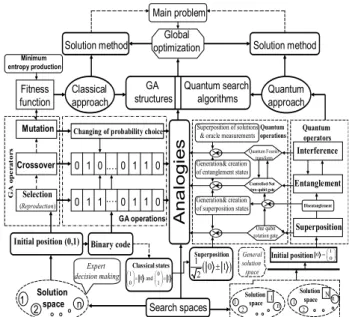
Figure 2 demonstrate the computing analogy between

soft and quantum algorithms and its operators that are used in quantum soft computing information technology.

Superposition

n Interference

… Main problem

Solution method _optimizationGlobal Solution method GA

structures Quantum search algorithms

A nal ogi e s Search spaces Classical approach Fitness function Minimum entropy production Quantum approach Mutation Crossover Selection Initial position (0,1)

Changing of probability choice

0 1 0 0 1 1 0 .… 0 1 1 .… 0 1 1 0 Binary code Classical states 1 0 0 and 1 0 1  ₌  ₌         Superposition ( ) 1 0 1 2 ± Generation& creation of entanglement states Generation& creation of superposition states Superposition of solutions

& oracle measurements

Initial position 1 0 0   =     Solution space 2 1 _n Solution space 2 n 1 1 Quantum Fourier transform One qubit rotation gate Controlled-Not two-qubit gate Solution space 2 1 N (Reproduction) G A o p era to rs GA operations General solution space Quantum operators Quantum operations ⊗ Disentanglement ⊗ ⊗ ⊗ Expert decision making Entanglement

Figure 2. Interrelations between Soft and Quantum Oper

-ators in Genetic and Quantum Algorithms

From quantum programming a quantum computer point view there no exist currently the general methodology of

quantum computing and simulation of dynamic systems

but it was developed many proposals of quantum simula

-tors (see, for example, the large list of quantum simula-tors available on [https://quantiki.org/wiki/list-qc-simulators]).

Remark. The purpose of this article is concerned with

the problem of discovering new QAs. Same as D-Wave,

processor supercomputing processes in a quantum com-puter can be described as a synergetic union of hybrid

quantum / classical HW, and quantum SW with quantum

soft support of quantum programming.

Remark. To understand more clearly the fundamental

capabilities and limitations of quantum computation we are to discover efficient QAs for interesting engineering

problems as intelligent cognitive control systems. One the most important open problem in computer sci-ence is to estimate the possibility of quantum speed-up for the search of computational problems solution.

Oracular, or black-box, problems are the first exam

-ples of problems that can be solved faster with a quantum computer than with a classical computer. The computer in the black box model is given access to oracle (or a black box) that can be queried to acquire information about the problem. To find the solution to the problem using as few

queries to the oracle as possible is the computation goal

[11-13]_.

1.1 Goal and Problem Solving

This article consider the design possibility a family of quantum decision-making and search algorithms (QA’s)

(see, Fig. 1) that it is the background of quantum com

-putational intelligence for solving the problems of Big & Mining data, deep quantum machine learning (based on quantum neural network), global optimization in intelli

-gent quantum control (using quantum genetic algorithms) etc. (see, in details Pt II).

1.2 Method of Solution and Smart Toolkit

The presented method and relative hardware implements

matrix and algorithmic forms of quantum operators that

are used in a QA (entanglement or oracle operators, and interference operator as in second and third steps of QA implementation) that increasing computational speed-up with respect to the corresponding SW realization of a traditional and a new QSA. A high level structure of a generic entanglement block that uses logic gates as

analogy elements is described. Method for

perform-ing Grover interference without products is introduced

[14, 15]. QUANTUM ALGORITHM ACCELATOR

COMPUTING: SW / HW SUPPORT

A. General Structure of Quantum Algorithm

The problem solved by a QA can be stated in the sym -bolic form:

Input A function f: {0,1}n_→{0,1}m

Problem Find a certain property of function f

A given function f is the map of one logical state into

another and QA estimate qualitative properties of function f .

General description of QA on Fig. 3 is demonstrated

(physically the type of operator

U

F describes the

qualita-tive properties of the function

f

).

Figure 4 shows the steps of QA that includes almost

of described qualitative peculiarities of function f and

physical interpretation of applied quantum operators.

In the scheme diagram of Fig. 5 the structure of a QA

is outlined.

|x>

H

UF |0>

Input Superposition Entanglement Interference Output

H |0> INT .. . n |x> m _.. . .. . .. . h S S h h h Repeated k times .. . .. . M E A S U R E M E N T bit bit bit bit

Figure 3. General Description of QAG

Qualitative properties of function

Problem

Quantum Fourier

transformation Problem orientedoperator transformationHadamard

Answer _{QAG design}

Quantum oracle as black box

Coding of function properties Qualitative properties of function Classical input QC output SCO Quantum KB optimizer

(

Interference Quantum oracle Superposition

)(

) (

)

fin initial

ψ = _ _ ψ

Quantum massive parallel computing

Figure 4. General Structure of QA

Encoder f→F ; F→U_F f INPUT U_F Quantum Block Basis Vectors Decoder Answer OUTPUT Binary strings level Complex Hilbert space Map Table and

Interpretation Spaces

Figure 5. Scheme Diagram of QA - structure

As above mentioned QA estimates (without numerical computing) the qualitative properties of the function f. Thus with QAs we can study qualitative properties of function

f without quantitative estimation of function values. For example, Fig. 6 represents the general approach to Grover’ QAG design.

Figure 6. Circuit and Quantum Gate Representation of

As a termination condition criterion minimum-entropy

based method is adopted [13]_.

The structure of a QAG in Fig. 3 in general form de

-fined as following:

(

_n

)

h 1 _{n m}

F

QAG

=





Int

⊗

I U

⋅





+

⋅





H

⊗

S





₍₁₎

Where I is the identity operator; S is equal to I or H and

dependent on the problem description.

Fast algorithms design to simulate most of known QAs

on classical computers [15-17] _{and computational}

intelli-gence toolkit is following: 1) Matrix based approach; 2)

Model representations of quantum operators in fast QAs;

3) Algorithmic based approach, when matrix elements are

calculated on “demand”; 4) Problem-oriented approach, where we succeeded to run Grover’s algorithm with up to 64 and more qubits with Shannon entropy calculation (up to 1024 without termination condition); 5) Quantum algorithms with reduced number of operators

(entangle-ment-free QA, and so on).

Remark. In this article we describe briefly main blocks

[13-17] _{in Fig. 6: i) unified operators; ii) problem-oriented} operators; iii) Benchmarks of QA simulation on classical computers; and iv) quantum control algorithms based on quantum fuzzy inference (QFI) and quantum genetic al

-gorithm (QGA) as new types of QSA (see, more in details Part II of this article).

Let us consider matrix based and problem-oriented

approaches to simulate most of known QAs on classical

computers and small quantum computer.

I. Quantum operator’s description: SW&HW smart toolkit support

We consider from simulation viewpoint the structure of quantum operators as superposition, entanglement and

interference [14,16,18,19,23-26] _{in matrix based approach.}

Superposition operators of QA’s.

The superposition operator consists in general form of

the combination of the tensor products Hadamard

H

op-erators with identity operator

I

:

1 1

1 0

1

,

1

1

0 1

2

H

=









I

=









−









.

The superposition operator of most QAs can be ex

-pressed (see Fig. 3 and Eq. (1)) as:

1 1 n m i i

Sp

H

S

= =



 



= ⊗



 

⊗ ⊗





 



,

Where

n

and

m

are the numbers of inputs and of

outputs respectively. Numbers of outputs

m

as well as

structures of corresponding superposition and interference

operators in [12, 13] _{for different QAs presented.}

Elements of the Walsh-Hadamard operator could be

obtained as following:

( )

* / 2 / 2 , 1, if is even 1 1 1, if is odd 2 2 i j n n n i j i j H i j ∗ −    = = _   _{− ∗ (2)}

Where_i=0,1,...,2 ,n _j=0,1,...,2n_{. Its elements could be}

obtained by the simple replication according to the rule

presented in Eq. (2).

Interference operators of main QA’s

Interference operators for Grover’s algorithm [18, 19] _writ

-ten as a block matrix:

/2 , /2 /2 /2 1 2 , 1 1 1 1 , , 2 2 2 Grover n n n i j n n n i j i j Int D I I I I i j I I I i j = ≠     = ⊗ =_ − _⊗ =   _{ } − =  _{− +} _⊗  _{⊗ =}      _≠      , (3) where _i=0,...,2 1,n_{− j=}0,...,2 1n_{− ,} n D refers to diffu-sion operator:

[ ]

1 ( ) / 2 , ( 1) 2 AND i j n i j n

D = − = [4,8]_{. Note that with}

bigger number of qubits, gain coefficient will become

smaller.

Entanglement operators of main QA’s

Operators of entanglement in general form are the part

of QA and the information about the function (being ana

-lyzed) is coded as “input-output” relation. In the general

approach for coding binary functions into corresponding entanglement gates arbitrary binary function considered as: f: 0,1{ }n→{ }0,1 ,m _{such that} f x( ,...,₀ xn−₁) ( ,...,= y₀ ym−₁)

. Firstly irreversible function f transfer into reversible function _F, as following: _F: 0,1

{ }

m n+ _→

{ }

0,1m n+ ,

and

(

0,..., n1, ,...,0 m1

)

( ,...,0 n1, ( ,...,0 n1) ( ,...,0 m1))

F x x− y y− = x x− f x x− ⊕ y y− ,

where

⊕

denotes addition modulo 2. This transfor -mation create unitary quantum operator and performs the

similar transformation. With reversible function

F

it is

possible design an entanglement operator matrix

accord-ing to the followaccord-ing rule:

[U

F

]

_iB_{, j}B =1 ( )iff F jB =iB, ,i j∈ 0,..,0;1,..,1; 

 

n m+ n m+ 

B denotes binary coding.

A diagonal block matrix of the form:UF=

            M 0 0  M 0 2 1n− is actually resulted entanglement operator.

Each block , 0,...,2 1n i

M i= − _{, can be obtained as fol}

-lowing 1 0 , iff ( , ) 0 , iff ( , ) 1 m i _k I F i k M C F i k − = =  = ⊗  ₌  (4)

And consists of

m

tensor products of

I

or of

C

op-erators, where

C

stays for NOT operator.

Note that entanglement operator (4) is a sparse matrix

and according to this property, the simulation of entangle -ment operation accelerated.

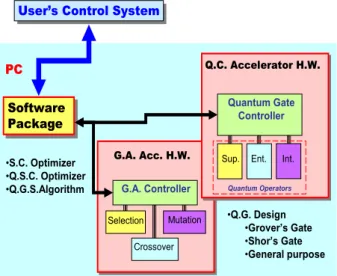
II. QA computing accelerator: SW&HW support Figure 7 shows the structure of intelligent quantum

computing accelerator. Software Package Software Package PC •S.C. Optimizer •Q.S.C. Optimizer •Q.G.S.Algorithm •Q.G. Design •Grover’s Gate •Shor’s Gate •General purpose Selection Crossover G.A. Controller Mutation

G.A. Acc. H.W. _{Sup. Ent. Int.}

Quantum Gate Controller

Quantum Operators Q.C. Accelerator H.W.

User’s Control System

User’s Control System

Figure 7. Intelligent Quantum Soft Computing Accelera

-tor Structure

HW of quantum computing accelerator is based on

standard silicon element background.

QA structure implementation for HW and MatLab is on Fig. 8 demonstrated (see, Fig. 23).

a Out put Input Background of HW implementation Int ellig ent co m pu ta tio n op er at or s Digital computation of Shannon entropy Stop Criterion Super pos itio n Int er fer en ce Ent ang lem ent Pre-In ter

Figure 8. QA Structure Presentation for HW (a) and Mat

-Lab (b) Implementations

Different structures of QA can be realized as shown in Table 1 below.

Table 1. Quantum Gate Types for QA’s Structure Design

Title Type of Algorithm

Symbolic Form of QAG:

( ) _ 1 h m n m F Superposition Entanglement Interference Int I U H S +   _{ }  _{⊗ ⋅}  _{⋅ ⊗ }     _{ }      Deutsch-Jozsa (D. – J.) m=1, S=H(x=1) Int=n_H k=1 h=0

(

)

(

)

. . 1 n D J n F H I U_{⊗ ⋅} − _⋅ +H Simon (Sim) m=n,S=I (x=0)Int=n_H k=O(n) h=0

(

)

(

)

n n Sim n n F H⊗ I U⋅ ⋅ H⊗ I Shor (Shr) m=n, S=I (x=0)Int=QFTn k=O(Poly(n)) h=0

(

)

(

)

n Shr n n n F QFT⊗ I U⋅ ⋅ H⊗ I Grover (Gr) m=1, S=H(x=1) Int=Dn k=1, h=O(2n/2₎

(

)

(

)

1 Gr n n F D _{⊗ ⋅}I U _⋅ +H 1.3 Information Analysis of QA and Criterion for Solution of the QSA-termination Problem

The communication capacity gives an index of efficiency

of a quantum computation [19]_{. The measure of Shannon}

information entropy is used for optimization of the termi

-nation problem of Grover’s QSA. Information analysis of Grover’s QSA based on of Eq. (5), gives a lower bound on

necessary amount of entanglement for searching of

suc-cess result and of computational time: any QSA that uses

the quantum oracle calls

{ }

Os as I−2s s must call the

oracle at least 1 1 2 e log P T N N π π  −  ≥_ + _   times to achieve a probability of error Pe [20].

The information intelligent measure of QA as ℑT

( )

ψ

of the state ψ is [12, 21]_:

( )

1

( )

( )

. Sh VN T T T S _TS

ψ

ψ

ψ

− ℑ = − (6)

With respect to the qubits in T and to the basis

{

1 n

}

B= i ⊗ ⊗_ i

The measure (6) is minimal (i.e., 0) when

( )

Sh T S y =T _and VN

( )

0 T S y = _{, it is maximal (i.e., 1)}

whenSTSh

( )

y =STVN

( )

y . Thus the intelligence of the QA

state is maximal if the gap between the Shannon and the von Neumann entropy for the chosen result qubit is mini -mal.

Information QA-intelligent measure (6) and interrela

-tions between information measures in Table 1 are used together with the step-by-step natural majorization

princi-ple for solution of QA-termination problem and interrela

-tions between information measures Sh

( )

VN

( )

T T

S ψ ≥S ψ _are

used together with entropic relations of the step-by-step natural majorization principle for solution of QA-termi

-nation problem [12]_{. From Eq. (6) we can see that (for pure} states)

( )

( )

( )

max 1 min Sh VN T T T S _TS ψ ψ ψ  −  ℑ −     

( )

( )

minS_TSh ψ , S_TVN ψ =0  _{, (7)}

i.e. from Eq. (6) the principle of Shannon entropy min

-imum is as follows.

Figure 9 shows digital block of Shannon entropy min -imum calculation and the main idea of the termination

criterion based on this minimum of entropy [13, 14]_.

(a)

b

Scheme background for SW implementation

Search space

of solutions Intelligent computation _operators

Information stopping criteria Measurement of result SW additional functions (b)

Figure 9. Digital Block of Shannon Entropy Minimum

Calculation (a) and MatLab (b) Implementations Number of iterations of QA defined during the calcula -tion process of minimum entropy search.

The structure of HW implementation of main quantum

operators.

Figure 10 shows the structure of superposition and in -terference operator simulation.

Shor Grover Deutsch-Jozsa Common Part Superposition Operator Quantum Algorithm 1 1 n+_{H H H= ⊗}n 1 1 n+_{H H H= ⊗}n n_{H I H I⊗ = ⊗}n n n n_H n_H n_H Shor Grover D.-Jozsa Common Part Interference Operator Quantum Algorithm ( ) 0 phase n n n QFT⊗I ⇒= H I⊗ n D I⊗ = H I⊗ H I⊗ H I⊗ n_{H I n H I⊗ = ⋅ ⊗} 1 0 0 0 0 1 0 0 0 0 1 0 0 0 0 1 n n H H I × ₋                      − ⊗           Sup. Int. I ⊗ n H Level 1 Level 2 Level 3 Software Software Hardware n H⋅ H I⊗ Controller

Figure 10. Computation of Superposition and Interference

Operators

The superposition state is created by appli -cation of Hadamard matrix to column vector

as

[

]

(

)

T 1 1 0 1 1 0 1 1 0 1       − =_{     }= + = − − −       . According to

this rule of quantum computing the superposition

model-ing circuit is developed [16]_.

Figure 11 shows the superposition modeling circuit.

The first operations needed are H|0>, H|0> and H|1>. Neglecting the factor 1/20.5_{, it can be} written:

H UF |0>

Input SuperpositionEntanglement

H |0> . . . n |1> H . . . h11=1 1 1+ + + --h21=1 1 |h22|=1 0 1 0 h12=1 0 0 [1 --1] T |0> |0>             − ⊗             − ⊗             −1 01 11 11 01 11 11 10 1 1 1

Direct product can be performed via AND gates. In fact

(2 qubits)

Final superposition state

0 ) 0 1 ( 0 * 1 ; 1 ) 1 1 ( 1 * 1 ; 1 1 1 1 * 1 = ∧ = − =− ∧ =− = ∧ =

Figure 11. Superposition (Qubit) Modeling Circuit

Qubits simulation circuits with tensor product on Fig. 12 is shown.

Note: no multipliers are introduced 2-qubit superposition 1 0 1 1 1 1 0 0 1 0 1 1 0 0                           = 0 1 0 1 0 1 0 1 1 0 1 1 1 1 0 0             = 0 1 0 1       = ⊗             = ⊗       0 0 1 or 1 1 A A A A A 3-qubit superposition

Figure 12. Qubits Simulation Circuits with Tensor Prod

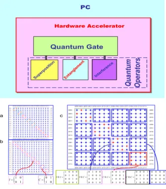
Figure 13 shows the computation of entanglement op -erators. PC Supe rposit ion Entan gleme nt Interf erence Quantum Gate Hardware Accelerator Qua nt um Ope ra to rs a c

Entanglement operators of quantum algorithms: a -Deutsch-Jozsa’s; b –Grover’s; c –Shor’s

b       = 1 0 0 1 I =_ _ 0 1 1 0 C             = ⊗ 1 0 0 0 0 1 0 0 0 0 1 0 0 0 0 1 I I             = ⊗ 0 1 0 0 1 0 0 0 0 0 0 1 0 0 1 0 C I             = ⊗ 0 0 1 0 0 0 0 1 1 0 0 0 0 1 0 0 I C             = ⊗ 0 0 0 1 0 0 1 0 0 1 0 0 1 0 0 0 C C             0 0 0 0 0 0 0 0 0 0 0 0 0 0 0 0

Figure 13. The Computation of Entanglement Operators

Figure 14 shows the entanglement creation circuit.

f(x) 0 1 0 0

Idea: to avoid encoding steps by acting directly on entanglement output vector via function f.

The output of entanglement can be realized by using couples of XOR gates:

g1 g2 g3 g4 g5 g6 g7 g8

00 01 10 11

y1 y2 y3 y4 y5 y6 y7 y8

Superposition Output Entanglement Output

Figure 14. The Entanglement Creation Circuit

Thus it is possible to obtain output of entanglement

G=UF ×Y without calculate matrix product and have only

knowledge of corresponding row of diagonal UF matrix

(see, Fig. 13).

Finally output vector

G

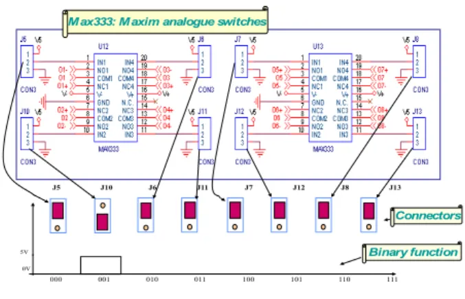
can write as following (Fig. 15):     _{= + + −} = , 0 ) 1 ( 2 1 ) ( , 2 1 2 / elsewhere j x f i if g n j n i 11 C⊗C Forn= 2 10 01 00 f(x) C⊗I I⊗C I⊗I Mi Example ofU_F

Figure 15: Equivalent form of Output Vector G

.

000 001 010 011 100 101 110 111

5V 0V

J5 J10 J6 J11 J7 J12 J8 J13

Max333: Maxim analogue switches

Connectors Binary function

Figure 16. Entanglement Circuit Realization

Figure 17 shows the circuit realization of interference operator according to the scheme in Fig. 10.

I-b:

Pre – interference

.

Let us consider the output V of

the entanglement block.

V=[v1 v2…… vi…… v2n+1]

In fact, if Y is the interference

output vector, its elements y_iare

TL081 OPAMP

(not implemented, being even = -odd)        − − =

∑

∑

= − = − − even i for v v odd i for v v y i j j n i j j n i n n , 2 1 , 2 1 2 1 2 1 2 1 2 1 1 I-c:Interference . TL084 OPAMP (not implemented, being even = -odd)

       − − =

∑

∑

= − = − − even i for v v odd i for v v y i j j n i j j n i n n , 2 1 , 2 1 2 1 2 1 2 1 1 2 1 ith_element processing unit Inti vi yi

Figure 17. Interference Circuit Realization

Let us consider briefly applications of QAG design ap

-proach in highly structured QSA; and in AI, informatics,

computer sciences and intelligent control problems (see

Part II).

SIMULATION OF QA - COMPUTING ON CLAS-SICAL COMPUTER

We discuss the general outline of the Grover’s QAs us

-ing the quantum gate (QAG) as

(

)

h

(

1

)

Gr n

n F

QAG

=



D

⊗ ⋅

I U



⋅

⊗ +

H





(7)

General method design of QAGs in [13, 14] _{is developed}

and is briefly described.

Figure 18a represents QAG of Grover’s algorithm (7) as control system, and Fig. 18b describe a general struc

-ture scheme of Grover's QSA (see, Fig. 1 and Table 1) [13]_.

0 1 n ⊗ Superposition 1 n _H ⊗ + Information Source Unmarked States Entanglement F U Quantum Oracle R.S.

ε

Information Optimization Wise Controlleru* Termination Interference n D ⊗I Control Object

Local Control Feed-back

Global Information Feed-back

POV Measure Measurement Process Decision-Making Feed-Forward Answer Information Comparator Physical Comparator Marked States min( ) Sh vN S −S Qualitative Properties Initial States POV: Positive Operator-Valued (a)

Grover Quantum Gate

The output is Φ = [(Dn⊗I) ⋅UF]h⋅(n+1H)       − = ₁1 1₁ 2 1 H              =       = 1 0 1 0 1 0 1 0 1 0 c c i = + ϕ Basis qubits    ≠ = − = −₋ j i j i dij n_n1 1 2 / 1 1 2 / 1 With: |1> H UF |0>

INPUT STEP 1 STEP 2 STEP 3 OUTPUT

H H |0> Dn .. . n h h h bit bit bit (b)

Figure 18. General Structure Scheme of Grover QSA

The Hadamard gates (Step 1) are the basic components for the superposition operation, the operator

U

F (Step 2)

performs entanglement operation and

D

n (Step 3) is the

diffusion matrix related to the interference operation. Our

composed of classical gates AND, NAND, XOR etc.) that simulate the quantum operations of Grover QSA. To this

aim all quantum operators must be expressed in terms of functions easily and efficiently described by classical

components. When we try to make the HW components

that perform this basic operations according to the

classi-cal scheme we encounter two main difficulties.

High-level gate design of Grover’s QSA (Model

based approach)

In this section we present a new model based HW im

-plementing the functional steps of Grover’s QSA from a high-level gate design point of view. According to the high-level scheme in Eq. (7) introduced in Fig. 4, the pro

-posed circuit can be divided into two main parts.

Part I: (Analogue) Step-by-step calculation of output

values. This part is divided into the following subparts:

I-a: Superposition; I-c: Pre-Interference (for vector’s approach);

I-b: Entanglement; I-d: Interference

Part II: (Digital) Entropy evaluation, vector storing for

iterations and output visualization. This part also provides

initial superposition of basis vectors

0

and

1

.

Figure 19 shows a general structure scheme of the HW realization for the Grover’s QSA-circuits and itself can be

considered as a classical prototype of intelligent control quantum system.

Figure 19. A General HW-scheme of the Grover’s QSA

Example. The most interesting novelty involves the

structure of interference: in fact the generic element

v

i

(interference output) can be written in function of

g

i

(en-tanglement output) as the following

2 2 1 1 1 2 2 1 1 1 _, 2 1 _, 2 n n j i n j i j i n j g g for i odd v g g for i even − − = − =  −   =   ₋ 

∑

∑

₍₈₎

Figures 20a and 20b show the Simulink schematic de

-sign and circuit realization of superposition, entanglement and interference operator’s blocks of the Grover’s QAG.

I-a II I I-c I-b A nal ogu e P ar t Digital Part: Stop Criterion Minimum of Shannon entropy S upe rpos ed input M ai n boa rd Entanglement Interference CPLD Board

Figure 20a. Simulink Scheme of 3-qubits Grover Search

System Superposition Superposition Entanglement Entanglement In te rf er en ce In te rf er en ce Pre

Pre--InterferenceInterference

Figure 20b. Pre Prototype Scheme Circuit of Grover’s

QAG

Referring to Fig. 19, pre-interference operation evalu

-ates a weighted sum of odd (even) output elements of en

-tanglement, while interference itself uses this contribution in order to provide (by means of difference with

g

i) the

respective

v

i. This simple (but powerful) result in Eq. (8)

has several consequences.

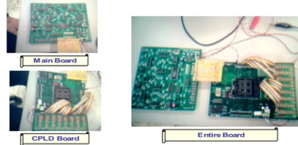
Figure 21 shows experimental HW evolution of Gro -ver’s quantum search algorithm for three qubits.

Main Board

CPLD Board Entire Board

Remark. Regarding to speed-up of computation, a

great improvement has been provided due to the smaller number of products (only one for each element of the

out-put vector) and more precisely

2

n+1 _against

4

n+1 _{of the}

classical approach. Also additions are less than 2 2 1n

(

n+

)

instead of

4

n+1_{). But the most important fact is that all}

these operation can be easily implemented in HW with few operational amplifiers

(

2n+2

)

.

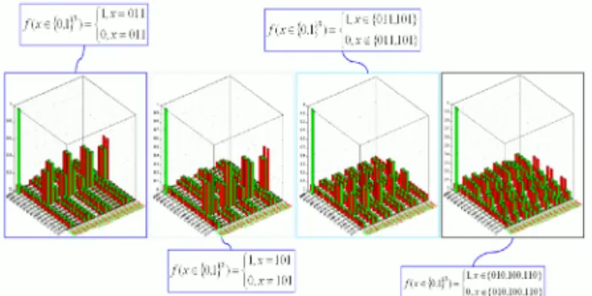
Example. Figure 22a - d shows the experimental

probability evolution of finding each of the database’s

elements (from Iteration #1 - to Iteration #4). At this step (Iteration #2) the probabilities of finding one of the 8 ele

-ments of the database are comparable. In the following

Figure 22. Experimental Results of 3-qubits HW-imple

-mentation of Grover’s QSA

Figure 23 shows the result of entropy analysis for Gro

-ver’s QSA according to Eq. (6), case n=7,f x

( )

0 =1.

Figure 23. Shannon Entropy Simulation of QSA with 7-

inputs

In Fig. 22c the probability of finding the second ele

-ment of the database begins to increase with respect to the probabilities of finding the others elements. After some other iterations of the algorithm, the difference between

the probability of finding the second element and the

probabilities to find the others is increased. Finally the

probability of extracting the second element of the

data-base is greater than the probabilities of finding any other elements. Figures 22b, 22c and 22d show the evolution of quantum searching using Grover’s QAG. It is a clear demonstration of how we can perform Grover’s algorithm

by a classical computer. Similar approach can be used for the realization of quantum fuzzy computing [27]_.

Application of Grover’s QAG is classical efficient sim

-ulation process for realization of quantum search compu

-tation on classical computer (see in details [17]_).

QUANTUM ALGORITHM ACCELATOR COMPUT

-ING: SW SUPPORT: EXAMPLES (matrix approach) The software system into two general sections is divid

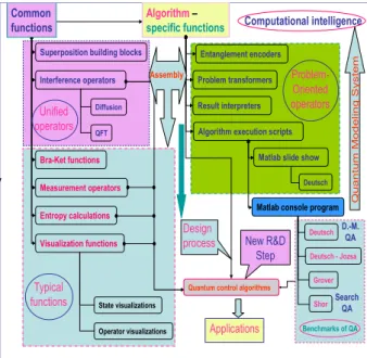
-ed (see, Fig. 24). Search QA Computational intelligence Q uant u m M odel in g S ys te m Algorithm– specific functions

Superposition building blocks

Bra-Ket functions Measurement operators Entropy calculations Visualization functions State visualizations Operator visualizations Entanglement encoders Interference operators Result interpreters Problem transformers Diffusion QFT

Matlab slide show

Deutsch

Matlab console program

Deutsch Deutsch - Jozsa

Shor Grover

Algorithm execution scripts

Quantum control algorithms

Benchmarks of QA Typical functions Problem-Oriented operators Applications Design process Unified operators D.-M. QA New R&D Step Assembly Common functions

Figure 24. Structure of QFMS and SW Toolkit

The first section involves common functions. The sec

-ond section involves algorithm-specific functions for real

-izing the concrete algorithms.

Figure 25 shows of quantum mechanical representation in SW of (bra – ket) vectors and calculation of quantum

states as density matrices. Quantum-mechanics

bra-ket definitions Density

matrix computing Fidelity Cla ssic al ope rati ons Quantum ope ration SW implem entation

Figure 25. SW Representation of Density Matrix and

Fidelity Calculation

Example: Quantum Shor’s Algorithm (Quantum

facto-rization promise). Figure 26 shows the factorization prob

-lem. Figure 27 shows the quantum Shor algorithm and its describing circuit (see Table 1). We can observe UF block

that is a diagonal matrix of

2

2n

×

2

2n _{dimension. Final}

block composed of Quantum Fourier Transform (QFT)

and identity matrix I. The output of entire algorithm is

therefore the vector obtained after application of opera-torQFTn⊗nI. 1. Classical factorization - 1024 bits: 105_years - 2048 bits: 5x1015_years - 4096 bits: 3x1029_years 2. Quantum factorization •1024 bits: 4.5 min •2048 bits: 36 min •4096 bits: 4.8 hours

Fast integer numbers Factorization

Figure 26. Fast Factorization Problem and Its Solutions

Entanglement and interference operators UF, QFT for Shor Algorithm

      − = 1 1 1 1 2 1 H

Figure 27. Quantum Shor’s Algorithm Circuit and Main

Quantum Operators

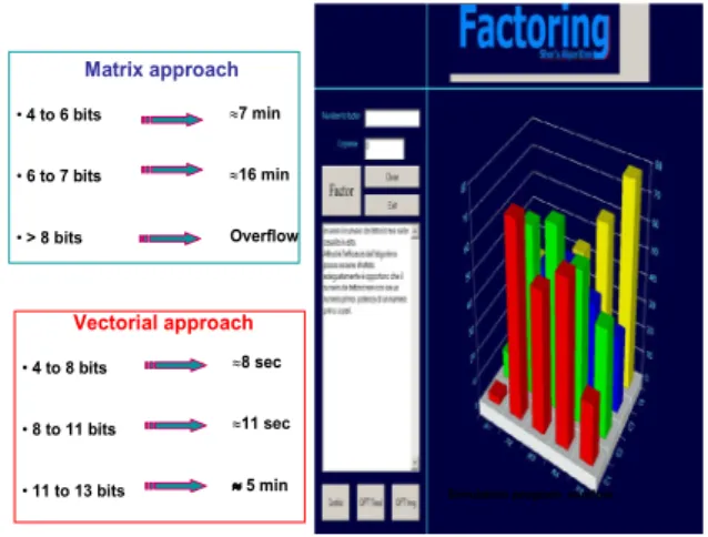
Factorization time using matrix and vector approach are here reported (see, Fig. 28).

Matrix approach Vectorial approach •4 to 8 bits •8 to 11 bits •11 to 13 bits ≈8 sec ≈11 sec ≈5 min •4 to 6 bits •6 to 7 bits •> 8 bits ≈7 min ≈16 min Overflow

Simulation program window

Figure 28. SW Simulation of Shor’s Quantum Factoriza

-tion Algorithm

Example: Command line simulation of the Grover’s

quantum search algorithm The example of the Grover’s

algorithm script is presented in Figs 29 and 30.

Figure 29. Example of Grover Algorithm Simulation

Script (Visualization of the Quantum Operators Sp, Ent,

Int and G = (Int)(Ent)(Sp))

Figure 30. Example of Grover Algorithm Simulation

Script (Visualization of the Input and of the Output Quan

-tum States)

In Fig. 29, the algorithm-related script is presented. It prepares the superposition (SP), entanglement (ENT) and interference (INT) operators of the Grover’s algorithm with 3 q-bits (including the measurement q-bit). Then it

assembles operators into the quantum gate G.

Then the script creates an input state in = 001 and

calculates the output state out = ×G in . The result of

this algorithm in Matlab is an allocation of the operator

matrices and of the state vectors in the memory. Code displays the operator matrices in Fig. 29 in 3D visualiza -tion. In this case the vertical axis corresponds to the am-plitudes of the corresponding matrix elements. Indexes of

the elements are marked with the ket notation. Input |in> and the output |out> states are demonstrated in Fig. 25. In this case, the vertical axis corresponds to the probability amplitudes of the state vector components. The horizontal

axis corresponds to the index of the state vector

compo-nent, marked using the ket notation.

The title of the Fig. 30 contains the values of the Shan

-non and of the von Neumann entropies of the correspond

Other known QA can be formulated and executed using similar scripts, and by using the corresponding equations taken from the previous section.

Simulation of QAs as dynamic control system

In order to simulate behavior of the dynamic systems

with quantum effects, it is possible to represent the QA as a dynamic system in the form of a block diagram and then simulate its behavior in time. Figure 31 is an example of a Simulink diagram of the quantum circuit for calculation of the fidelity a a of the quantum state and for the

calcula-tion of the density matrix a a of the quantum state. Bra

and ket functions are taken from the common library. This

example demonstrates the usage of the common functions

for the simulation of the QA dynamics.

In Fig. 31, input is provided to the ket function. The output of the ket function is provided to the first input of

the matrix multiplier and as a second input of the matrix

multiplier. Input is also provided to the bra function. The

output of the bra function is provided to the second input

of the matrix multiplier and as a first input of the matrix

multiplier. Output of the multiplier is a density matrix of

the input state. Output of the multiplier is the fidelity of

the input state.

Figure 31. Simulink Diagram for the Simulation of the

Arbitrary Quantum Algorithm

Figure 32 shows Simulink structure of an arbitrary QA. Such a structure can be used to simulate a number of quantum algorithms in Matlab / Simulink environment.

Figure 32. Simulink Diagram for the Simulation of the

Arbitrary QA

Simulation result of Grover’s QSA on Fig. 33 is shown.

Figure 33. Evolution of Grover’s Quantum Search Algo

-rithm: Quantum Simulator on Classical Computer (Matrix Approach)

Dynamic evolution of successful results of algorithm

execution for the first iteration of Grover’s QAG for initial

qubits state 0001 and different answer search is shown

in Fig. 34.

Figure 34. Grover’s QSA: Algorithm Execution [First

Iteration]

Figure 35 shows algorithm execution results for Gro

-ver’s QSA with different number of iterations for success

-ful results with different searching answer number.

Figure 35. Grover’s QA: Step 2. Algorithm Execution

Figure 36 is a 3D dynamic representation of Grover’s QAG probabilities evolution (step 2 of Fig. 33) for differ

-ent cases of answer search.

Figure 36. Grover’s QA: Step 2 [Algorithm Execution 3D

Dynamics: Probabilities]

Algorithm execution results of Grover’s QAG (step 2 of Fig. 33) with different stopping iteration for searching answers are shown in Fig. 35.

Example: Interpretation of measurement results in

simulation of Grover’s QSA-QAG.

In the case of Grover’s QSA this task is achieved

(according to the results of this section) by preparing

the ancillary qubit of the oracle of the transformation:

( )

: , , f U x a _ x f x ⊕a _{in the state} 0 1 0 1

(

)

2 a = − .

The operator I x0 is computationally equivalent to Uf:

( ) ( ) ( ) ( ) _ ( ) _ 0 0 0 1 _{0 1} 1 _{0 1} 2 2 1 ₀ 1 ₁ 2 2 f x x x Measurement Measurement Computation Result Computation Result

U x I x I x I x  _{⊗ −}  _{=  ⊗ −}           = _{ } ⊗ − _{ }⊗  

and the operator Uf is constructed from a controlled

0

x

I _{and two one qubit Hadamard transformations. Fig}

-ure 37 shows the interpretation of results of the Grover QAG.

Figure 37. Grover’s QA: Step 2 [Result Interpretation]

Measured basis vector is computed from the tensor

product between the computation qubit results and ancil -lary measurement qubit. In Grover’s searching process the ancillary qubit does not change during the quantum com-puting.

As described above operator

U

f is constructed from

two Hadamard transformations and the Hadamard trans

-formation H (modeling the constructive interference) ap

-plied on the state of the standard computational basis can

be seen as implementing a fair coin tossing. Thus, if the

matrix 1 1 1 1 1 2 H = _ _ −

  is applied to the states of the

stan-dard basis then _H2 _{0 = −1 , H}2 _{1 = 0 and therefore}

2

H acts in measurement process of computational result

as a NOT-operation up to the phase sign. In this case the

measurement basis separated with the computational basis (according to tensor product).

Figures 38 and 39 shows the measurement result and

final results of entropy dynamic evolution interpretation

of Grover’s QSA for search of successful results with different number of marked states (in computational basis

{

0 , 1

}

). These results represent the possibility of the classical efficient simulation of Grover’s QSA.

Figure 38. Interpretation of Measurement Results of QSA

Figure 39. Shannon Entropy Dynamics after 31 Steps of

Grover’s QSA

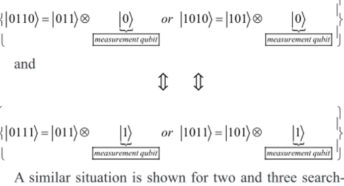
Remark. Figure 38 (b) shows the results of computation

on a classical computer and shows two possibilities:





0110

011

0

Result measurement qubit







=

⊗















and









0111

011

1

Result measurement qubit







=

⊗















.

Figure 38 (b) demonstrates also two searching marked states:

 

0110 011 0 1010 101 0

measurement qubit measurement qubit

or    _{= ⊗ = ⊗}        and





  0111 011 1 1011 101 1

measurement qubit measurement qubit

or    _{= ⊗ = ⊗}       

A similar situation is shown for two and three search

-ing marked states in Fig. 37 (b).

Using a random measurement strategy based on a fair

coin tossing in the measurement basis

{

0 , 1

}

one can

independently receive with certainty the searched marked

states from the measurement basis result.

The measurement results based on a fair coin tossing measurement are shown in Fig. 38 (c) and shows accurate results of searching of corresponding marked states. Figure 38 (c) shows also that for both possibilities in implementing

a fair coin tossing type of measurement process the search

for the answer is successful.

Final results of interpretation for Grover’s algorithm are shown in Fig. 38.

Let us describe briefly the main blocks in Fig. 2: i) uni

-fied operators; ii) problem-oriented operators; iii) Bench

-marks of QA simulation on classical computers; and iv) quantum control algorithms based on quantum fuzzy inference (QFI) and quantum genetic algorithm (QGA) as new types of QSA (see, Part II of this article).

Let us consider problem-oriented operators description. Problem-oriented approach based on structural pattern of

QA state vector with compressed vector allocation.

Let

n

be the input number of qubits. In the Grover

algorithm (as mentioned above) half of all

2

n+1 _elements

of a vector making up its even components always take values symmetrical to appropriate odd components and, therefore, need not be computed.

Odd

2

n_{elements can be classified into two categories:}

• The set of m elements corresponding to truth points of

input function (or oracle); and • The remaining

2

n

−

m

elements.

The values of elements of the same category are always

equal.

As discussed above, the Grover QA only requires two

variables for storing values of the elements. Its limitation in this sense depends only on a computer representation of

the floating-point numbers used for the state vector proba

-bility amplitudes. For a double-precision software realiza

-tion of the state vector representa-tion algorithm, the upper

reachable limit of q-bit number is approximately 1024 [13]_.

Figure 40 shows a state vector representation algorithm for the Grover QA.

Figure 40. State Vector Representation Algorithm for

Grover’ Quantum Search

Remark. In Fig. 40,

i

is an element index, f is an input

function, vx and va corresponds to the elements’ category,

and v is a temporal variable. The number of variables used

for representing the state variable is constant. A constant number of variables for state vector representation allow

reconsideration of the traditional schema of quantum search simulation.

Classical gates are used not for the simulation of ap

-propriate quantum operators with strict one-to-one corre -spondence but for the simulation of a quantum step that changes the system state. Matrix product operations are

replaced by arithmetic operations with a fixed number of

parameters irrespective of qubit number.

Figure 41 shows a generalized schema for efficient simulation of the Grover QA built upon three blocks, a superposition block H, a quantum step block UD and a

termination block T.

Figure 41. Generalized Schema of Simulation for Grover’

QSA

block.

Remark. The UD block includes a U block and a D

block. The input state from the input block is provided to the superposition block. A superposition of states from the

superposition block is provided to the U block. An output

from the U block is provided to the D block. An output

from the D block is provided to the termination block. If

the termination block terminates the iterations, then the state is passed to the output block; otherwise, the state

vector is returned to the U block for iteration.

As shown in Fig. 42, the superposition block H for

Grover QSA simulation changes the system state to the

state obtained traditionally by using n + 1 times the tensor product of Walsh-Hadamard transformations. In the

pro-cess shown in Fig. 41, vx:= hc, va:= hc, and vi:= 0, where

hc = 2 - (n+1) / 2 _{is a table value.}

Figure 42. Superposition Block for Grover’s QSA

The quantum step block UD that emulates the

entan-glement and interference operators is shown on Figs 43 (a

- c).

Figure 43 (a). Emulation of the Entanglement Operator

Application of Grover’s QSA

Figure 44 (b). Emulation of Interference Operator Appli

-cation of Grover’s QSA

Figure 44 (c). Quantum Step Block for Grover’ Quantum

Search

The UD block reduces the temporal complexity of the

quantum algorithm simulation to linear dependence on the

number of executed iterations. The UD block uses recal

-culated table values dc1 =

2

n

−

m

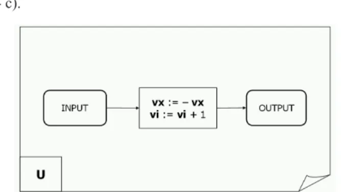
and dc2 = 2 n-1_.

Remark. In the U block shown in Fig. 44 (a), vx:= - vx

and vi:= vi + 1. In the D block shown in Fig. 44 (b), v:=

m*vx+dc1*va, v:= v/dc2, vx:= v - vx, and va:= v - va in

the UD block shown in Fig. 44 (c), v:= dc1*va = m*vx,

v:=v/dc2, vx:=v + vx, va:= v - va, and vi:= vi + 1.

The termination block T is general for all QAs, in

-dependently of the operator matrix realization. Block T provides intelligent termination condition for the search

process. Thus, the block T controls the number of

itera-tions through the block UD by providing enough itera-tion to achieve a high probability of arriving at a correct

answer to the search problem. The block T uses a rule based on observing the changing of the vector element

values according to two classification categories. The T

block during a number of iterations, watches for values

of elements of the same category monotonically increase

or decrease while values of elements of another category

changed monotonically in reverse direction. If after some

number of iteration the direction is changed, it means that an extremum point corresponding to a state with maxi

-mum or mini-mum uncertainty is passed. The process can

using direct values of amplitudes instead of considering

Shannon entropy value, thus, significantly reducing the

required number of calculations for determining the mini-mum uncertainty state that guarantees the high probability

of a correct answer.

The termination algorithm realized in the block T can

be used one or more of five different termination models:

o Model 1: Stop after a predefined number of iterations;

o Model 2: Stop on the first local entropy minimum;

o Model 3: Stop on the lowest entropy within a pre

-defined number of iterations;

o Model 4: Stop on a predefined level of acceptable en

-tropy; and/or

reachable entropy within the predefined number of itera -tions.

Note that models 1 - 3 do not require the calculation of

an entropy value.

Figures 45 – 47 show the structure of the termination condition blocks T.

Figure 45. Termination Block for Method 1

Figure 46. Component B for the Termination Block

Figure 47 (a). Component PUSH for the Termination

Block

Figure 47 (b). Component POP for the Termination Block

Since time efficiency is one of the major demands on such termination condition algorithm, each part of the ter

-mination algorithm is represented by a separate module, and before the termination algorithm starts, links are built between the modules in correspondence to the selected termination model by initializing the appropriate func -tions’ calls.

Table 2 shows components for the termination condi

-tion block T for the various models. Flow charts of the termination condition building blocks are provided in Figs

45 – 50

Table 2. Termination Block Construction

Model T B’ C’ 1 A -- --2 B PUSH --3 C A B 4 D -- --5 C A E

The entries A, B, PUSH, C, D, E, and PUSH in Table 2 correspond to the flowcharts in Figs 40 – 45 respectively.

Figure 49. Component D for the Termination Block

Figure 50. Component E for the Termination Block

Remark: Peculiarities of QA termination models in

model 1, only one test after each application of quantum

step block UD is needed. This test is performed by block

A. So, the initialization includes assuming A to be T, i.e.,

function calls to T are addressed to block A. Block A is

shown in Fig. 45 and checks to see if the maximum num

-ber of iterations has been reached, if so, then the simula

-tion is terminated, otherwise, the simula-tion continues.

In model 2, the simulation is stopped when the direc

-tion of modifica-tion of categories’ values are changed. Model 2 uses the comparison of the current value of vx

category with value mvx that represents this category val-ue obtained in previous iteration:

(i) If vx is greater than mvx, its value is stored in mvx,

the vi value is stored in mvi, and the termination block

proceeding to the next quantum step;

(ii) If vx is less than mvx, it means that the vx maximum

is passed and the process needs to set the current (final)

value of vx: = mvx, vi := mvi, and stop the iteration pro

-cess. So, the process stores the maximum of vx in mvx and

the appropriate iteration number vi in mvi. Here block B,

shown in Fig. 46 is used as the main block of the termina -tion process.

The block PUSH, shown in the Fig. 47 (a) is used for

performing the comparison and for storing the vx value in

mvx (case a). A POP block, shown in Fig. 47 (b) is used

for restoring the mvx value (case b). In the PUSH block

of Fig. 47 (a), if |vx| > |mvx|, then mvx: = vx, mva: = va,

mvi: = vi, and the block returns true; otherwise, the block

returns . In the POP block of Fig. 47 (b), if |vx| <= |mvx|,

then vx: = mvx, va:= mva, and vi:= mvi.

The model 3 termination block checks to see that a pre

-defined number of iterations do not exceed (using block A

in Fig. 43):

• If the check is successful, then the termination block

compares the current value of vx with mvx. If mvx is less

than, it sets the value of mvx equal to vx and the value of

mvi equal to vi. If mvx is less using the PUSH block, then

perform the next quantum step;

• If the check operation fails, then (if needed) the final

value of vx equal to mvx, vi equal to mvi (using the POP

block) and the iterations are stopped.

The model 4, the termination block uses a single com

-ponent block D, shown in Fig. 48. The D block compares the current Shannon entropy value with a predefined ac

-ceptable level. If the current Shannon entropy is less than the acceptable level, then the iteration process is stopped; otherwise, the iterations continue.

The model 5 termination block uses the A block to

check that a predefined number of iterations do not ex

-ceeded (see, Fig. 45). If the maximum number is exceed

-ed, then the iterations are stopped. Otherwise, the D block is then used to compare the current value of the Shannon entropy with the predefined acceptable level. If acceptable level is not attained, then the PUSH block is called and the iterations continue. If the last iteration was performed, the POP block is called to restore the vx category maximum and appropriate vi number and the iterations are ended.

Figure 51 shows measurement of the final amplitudes

in the output state to determine the success or failure of the search.

Figure 51. Final Measurement Emulation

If |vx| > |va|, then the search was successful; otherwise,

the search was not successful.

Table 3 lists results of testing the optimized version of Grover QSA simulator on personal computer with Penti

-um 4 processor at 2GHz.

Table 3 High Probability Answers for Grover QSA

Qbits Iterations Time

36 205887 0.018 40 823549 0.077 44 3294198 0.367 48 13176794 1.385 52 52707178 2.267 56 210828712 20.308 60 843314834 81.529 64 3373259064 328.274 Simulation results

The theoretical boundary of this approach is not the number of qubits, but the representation of the float

-ing-point numbers. The practical bound is limited by the front side bus frequency of the personal computer. Using the above algorithm, a simulation of a 1000 qubit Grover QSA requires only 96 seconds for 108 _iterations.

Figure 52 shows the simulation result of Grover’s algo

-rithm [problem-oriented approach with compressed vector

allocation] [14]_.

In less than 2 minutes

100 000 000 Iterations 1000 qubit Grover’s algorithm simulation ( 21000elements in DB)

Figure 52. Simulation Results of Problem Oriented

Grover’s QSA According to Approach 4 with 1000 Qubit (Simulator Window Snapshot)

The described method is differed from [23-44]_.

Let us discuss briefly the applications of QAG ap

-proach in design of new types of quantum search algo -rithm as quantum genetic algo-rithm.

Quantum fuzzy inference and quantum genetic algo

-rithm: Quantum simulator

Intelligent control systems (ICS) based on the use of soft computing, fuzzy logic, evolutionary algorithms and neural networks. Basis of management systems - propor

-tional–integral–derivative (PID) controller, which is used in 70% of the industrial automation, but often can`t cope with the task of managing and does not work well in un

-predicted control situations. The use of quantum comput

-ing and quantum search algorithms, as a special example, quantum fuzzy inference (QFI), allows increasing robust