Performance of IMERG as a Function of Spatiotemporal Scale
1Jackson Tan∗
2
Universities Space Research Association, and NASA Goddard Space Flight Center, Greenbelt, Maryland
3
4
Walter A. Petersen
5
Earth Sciences Office, ZP-11, NASA Marshall Space Flight Center, Huntsville, Alabama
6
Pierre-Emmanuel Kirstetter
7
School of Civil Engineering and Environmental Sciences, University of Oklahoma, Norman, Oklahoma, and NOAA/National Severe Storms Laboratory, Norman, Oklahoma
8
9
Yudong Tian
10
Earth System Sciences Interdisciplinary Center, University of Maryland, College Park, College Park, Maryland, and NASA Goddard Space Flight Center, Greenbelt, Maryland
11
12
∗Corresponding author address: Jackson Tan, NASA Goddard Space Flight Center, Code 613
Building 33 Room C327, 8800 Greenbelt Road, Greenbelt, MD 20771.
13
14
E-mail: [email protected]
15
ABSTRACT
The Integrated Multi-satellitE Retrievals for GPM (IMERG), a global high-resolution gridded precipitation data set, will enable a wide range of applica-tions, ranging from studies on precipitation characteristics to applications in hydrology to evaluation of weather and climate models. These applications focus on different spatial and temporal scale and thus average the precipita-tion estimates to coarser resoluprecipita-tions. Such a modificaprecipita-tion of scale will impact the reliability of IMERG. In this study, the performance of the Final run of IMERG is evaluated against ground-based measurements as a function of
in-creasing spatial resolution (from 0.1◦to 2.5◦) and accumulation periods (from
0.5 h to 24 h) over a region in the southeastern US. For ground reference, a product derived from the Multi-Radar/Multi-Sensor suite, a radar- and gauge-based operational precipitation dataset, is used. The TRMM Multisatellite Precipitation Analysis (TMPA) is also included as a benchmark. In general, both IMERG and TMPA improve when scaled up to larger areas and longer time periods, with better identification of rain occurrences and consistent im-provements in systematic and random errors of rain rates. Between the two satellite estimates, IMERG is slightly better than TMPA most of the time. These results will inform users on the reliability of IMERG over the scales relevant to their studies.
16 17 18 19 20 21 22 23 24 25 26 27 28 29 30 31 32 33 34
1. Introduction
35
Satellite retrievals of precipitation are instrumental in understanding the distribution of
precip-36
itation around the globe. In regions with sparse measurements, such as mountainous areas and
37
oceans, these remotely sensed estimates help to bridge gaps and constrain the errors in
ground-38
based data. This is typically achieved through the use of gridded high resolution precipitation
39
datasets, such as the Integrated Multi-satellitE Retrievals for GPM (IMERG; Huffman et al. 2015),
40
the TRMM Multisatellite Precipitation Analysis (TMPA; Huffman et al. 2007), Climate Prediction
41
Center morphing algorithm (CMORPH; Joyce et al. 2004; Joyce and Xie 2011), and Precipitation
42
Estimation from Remotely Sensed Information using Artificial Neural Networks Cloud
Classifi-43
cation Scheme (PERSIANN-CCS; Hong et al. 2004). These gridded precipitation datasets use a
44
blend of data from various sources with advanced techniques to provide a near-global coverage
45
with high spatial and temporal resolution.
46
However, to understand and benchmark the performances of these datasets, they need to be
47
evaluated against ground measurements. To this end, a whole range of ground validation efforts
48
have been undertaken to evaluate these datasets based on different criteria. Some studies focus on
49
different rain systems (e.g. Ebert et al. 2007; Habib et al. 2009; Roca et al. 2010; Mei et al. 2014).
50
Some studies analyze the performance by terrain or surface (e.g. Tian and Peters-Lidard 2007;
51
Kubota et al. 2009; Stampoulis and Anagnostou 2012; Chen et al. 2013b; Liu 2016). Some studies
52
investigate the downstream impact of the estimates on hydrologic modeling (e.g. Gottschalck et al.
53
2005; Xue et al. 2013; Falck et al. 2015; Tang et al. 2016b). Some studies focus on a better
54
understanding of the errors in these datasets themselves (e.g. Maggioni et al. 2014; Tang et al.
55
2015; Tan et al. 2016).
The aim of this study is to quantify the performance of IMERG as a function of spatial and
57
temporal scale. Similar analyses have been performed for other products. For example, Tian et al.
58
(2007) compared TMPA and CMORPH at daily, seasonal and annual time scales against ground
59
radar and gauges, finding that CMORPH is better at daily resolution while TMPA is superior at
60
the longer time scales. On the other hand, Hossain and Huffman (2008) examined the
sensitiv-61
ity of various metrics to spatial and temporal scale in PERSIANN-CCS against rain gauges, and
62
found that the probability of detection of rain is most sensitive to scale, followed by correlation
63
length. Gourley et al. (2010) evaluated TMPA and PERSIANN-CCS against a radar-based
prod-64
uct as a function of spatial scale, temporal scale and intensity, showing that TMPA is better than
65
PERSIANN-CCS, though both had reduced skill at higher intensities. Habib et al. (2012)
in-66
vestigated the performance of CMORPH against gauges and radar across a range of spatial and
67
temporal scales, with the conclusion that random error decreases with increasing scale. Sarachi
68
et al. (2015) proposed a statistical model to quantify the uncertainties in gridded satellite estimates
69
by deriving parameters to a generalized normal distribution as a function of scale.
70
In this study, we build on these studies and evaluate the IMERG Final run on its ability to identify
71
rain occurrences and rain rates over a range of spatial and temporal scales against a ground-based
72
dataset derived from the Multi-Radar/Multi-Sensor product over a region in the United States.
73
Our goal is to examine how various aspects of IMERG change as it is averaged over larger areas
74
and longer periods. For example, it is expected that random errors would decrease with more
75
averaging; indeed, our study will show that averaging the estimates in a 0.1◦grid box from 0.5 h
76
to 24 h will reduce the normalized root-mean-square error from 1.7 to 1.0. Hence, our results also
77
provide users with quantitative information on the performance of IMERG at a scale suitable to
78
their purposes.
2. Data
80
a. IMERG
81
The Integrated Multi-satellitE Retrievals for GPM (IMERG) is a gridded precipitation product
82
that merges measurements from a network of satellites in the GPM constellation (Huffman et al.
83
2015). IMERG uses the GPM Core Observatory satellite, which has a dual-frequency
precipita-84
tion radar and a 13-channel passive microwave imager, as a reference standard to intercalibrate
85
and merge precipitation estimates from individual passive microwave (PMW) satellites in the
con-86
stellation (Hou et al. 2014). Lagrangian time-interpolation is then applied to these estimates using
87
displacement vectors derived from infrared (IR) measurements on geosynchronous satellites to
88
produce gridded high resolution estimates of rainfall. This process, known as morphing, was first
89
introduced as the central component in CMORPH (Joyce et al. 2004; Joyce and Xie 2011). This
90
gridded estimate is further supplemented via a Kalman filter with microwave-calibrated rainfall
91
estimates calculated directly from IR measurements following the PERSIANN-CCS algorithm
92
(Hong et al. 2004). The final satellite estimate is then calibrated, either directly for the
post-93
real-time product or indirectly for the near-real-time products, using gauge data from the Global
94
Precipitation Climatology Centre monthly precipitation dataset following the approach employed
95
in TMPA (Huffman et al. 2007).
96
IMERG has a high resolution of 0.1◦ every half-hour covering up to ±60◦ latitudes. Three
97
choices of IMERG runs are available depending on user requirements. The Early run, available
98
at a 6-hour delay for real-time applications such as for hazard predictions, is limited to rainfall
99
morphing only forward in time. The Late run, with a 18-hour delay for purposes such as crop
100
forecasting, employs morphing both forward and backward in time. The Final run is at a 4-month
101
delay for research applications. Both the Early and Late runs have climatological gauge adjustment
while the Final run uses monthly gauge adjustments to reduce bias. Moreover, runs with longer
103
delays will use more PMW estimates due to latency in data delivery. Note that these delays will
104
eventually be reduced towards the targets of 4-hour, 12-hour and 2-month respectively. This study
105
focuses on the calibrated estimate from Final run of IMERG, which is available from Apr 2014
106
onwards.
107
Currently, IMERG ingests data from Version 3 of GPM, which uses algorithms implemented at
108
the launch of the GPM Core Observatory in Feb 2014 and is thus subject to further improvements
109
as measurements are collected. The release of an updated IMERG using Version 4 of the GPM
110
products is imminent and may involve potential improvements. We do not expect this new version
111
of IMERG to introduce major changes to the results of our study; however, should any significant
112
difference arise, we will address the changes in a follow-up paper. IMERG can be downloaded
113
from http://pmm.nasa.gov/data-access.
114
b. TMPA
115
The TRMM Multisatellite Precipitation Analysis (TMPA; also known as TRMM 3B42) is the
116
gridded precipitation product from the TRMM project. Just as with IMERG, TMPA uses the
117
TRMM satellite to calibrate and combine PMW estimates from different platforms. Estimates
118
derived from geosynchronous IR measurements calibrated against PMW estimates on a monthly
119
basis are used to fill in the gaps in the PMW field.
120
TMPA is available at a resolution of 0.25◦ every 3-hour covering up to ±50◦ latitudes. Two
121
different products of TMPA are available: the real-time product (with a 9-hour delay) and the
122
research product. This study uses the research product, which is available beginning 1998.
123
The research product utilizes the TRMM Precipitation Radar on board the satellite for
tion and has the additional monthly gauge adjustment step. TMPA can be downloaded from
125
http://pmm.nasa.gov/data-access.
126
Due to the decommissioning of the TRMM satellite, the TMPA research product switches, in
127
Oct 2014, from calibration with the Precipitation Radar to a climatological calibration modified
128
from the real time product. While this change may introduce a discontinuity from Sep to Oct
129
2014, the use of gauge adjustment should minimize, if not eliminate, artifacts for estimates over
130
land (Bolvin and Huffman 2015).
131
c. Reference
132
The Multi-Radar/Multi-Sensor (MRMS; formerly National Mosaic and Multi-Sensor QPE)
sys-133
tem is a gridded product by NOAA/NSSL based primarily on the US WSR-88D network (Zhang
134
et al. 2011b). Reflectivity data are mosaicked onto a 3D grid over the United States with quality
135
control for beam blockages and bright band. From the reflectivity structure and environmental field
136
at each grid point, a precipitation regime (e.g. snow, stratiform rain, convective rain) is determined
137
using physically-based heuristic rules and a corresponding reflectivity-precipitation relationship is
138
applied to estimate the surface precipitation rate. These precipitation rates are bias-corrected using
139
gauge data from the Hydrometeorological Automated Data System1and regional rain gauge
net-140
works. A radar quality index (RQI) is produced alongside each precipitation estimate in MRMS
141
(Zhang et al. 2011a), providing a numerical value that reflects sampling and estimation
uncer-142
tainty, such as beam issues relating to orography and bright bands. Evaluation of MRMS shows
143
better performances with the gauge correction and the quantitative benefit of the RQI filter (Chen
144
et al. 2013a; Kirstetter et al. 2015a).
145
For the analysis herein, we use a reference dataset processed from the MRMS suite in support
146
of the GPM mission for ground validation, available from Jun 2014 onwards (Kirstetter et al.
147
2012, 2014, 2015b; Gebregiorgis et al. 2016). This product aggregates the MRMS rain rates to
148
produce a half-hourly accumulated rain rates over the conterminous United States (20◦–55◦N,
149
130◦–60◦W) with a high spatial resolution of 0.01◦. For this reference product, the RQI ranges
150
from 0 (lowest quality) to 100 (highest quality). We mask pixels with RQI less than 100, thus
151
keeping only perfect-RQI pixels in computing the areal averages. A perfect RQI indicates an
152
absence of blockage and a radar beam below the bright band. We also exclude all pixels in which
153
frozen precipitation is identified. Thus, this study focuses only on the most reliable estimates of
154
liquid precipitation.
155
3. Approach
156
We restrict our analysis to 30.0–41.5◦N, 93.5–83.5◦W, a region within which the reference is
157
highly reliable due to good radar coverage, high density of gauges and absence of significant
158
orography. The RQI in this region is generally high (Fig. 1). This flat topography, together with a
159
lack of frozen surfaces at most times of the year, also means that satellite retrievals are generally
160
more accurate, though the reliance on ice scattering in retrievals over land will lead to challenges
161
in the estimation of warm rain. Within this region, we randomly sample an ensemble of 100
162
square boxes of length 0.1◦ and extract the IMERG and reference precipitation rates in each of
163
these boxes over the period of 19 months (Jun 2014 to Dec 2015). We then do the same for square
164
boxes of length 0.2◦ (i.e. 2 × 2 IMERG grid boxes), repeating it at 0.1◦ increments up to and
165
including 2.5◦. From these rates as a function of spatial scale, we average them to get rates over
166
periods of 1 h, 3 h, 6 h, 12 h and 24 h. This is also done separately for TMPA and the reference,
167
at increments of 0.25◦to 2.50◦ and periods of 3 h, 6 h, 12 h and 24 h. Therefore, for each spatial
and temporal scale, we have 100 sets of precipitation rates between IMERG and the reference as
169
well as TMPA and the reference, from which we can derive the statistics for each pair of rain rates
170
and take the average across the ensemble to reduce sampling bias. Note that we are working with
171
precipitation rate and not accumulated precipitation; in other words, the units of the precipitation
172
are mm / h over 1 hr, 3 hr, ... , 24 h instead of mm.
173
The period of this analysis covers 19 months over 2014 and 2015 without a distinction between
174
different seasons. Additional analyses for the warm season (Apr 2015 to Sep 2015) and the cold
175
season (Oct 2014 to Mar 2014) show that the difference is generally an offset in the performance
176
of IMERG, with the warm season slightly better than the cold season as consistent with previous
177
studies (Guo et al. 2016; Liu 2016). However, as the behavior of the performance as a function
178
of scale is generally similar between the two seasons, we will not distinguish between the two
179
seasons in the following sections. Instead, readers interested in the results for each season can
180
refer to the Supplementary Material.
181
We evaluate IMERG and TMPA against the reference on two aspects: (i) rain occurrences, i.e.
182
if they agree that it is raining above a certain threshold or not; and (ii) rain rates, i.e. when both
183
are raining, the degree to which the rates are similar. This follows the approach advocated in
184
Tang et al. (2015). As such, our analyses may depend considerably on the chosen threshold. This
185
presents an immediate challenge as rain rates are a function of scale, a situation well exemplified
186
in Fig. 2, which shows better agreement between IMERG and the reference at longer and larger
187
scales. While we expect rain rates to decrease with increasing scale due to coarsening, the fraction
188
of raining events actually increase, as demonstrated in Fig. 3 through a fixed threshold of 0.2 mm
189
/ h. This will have a bearing on the results because many aspects of rainfall evaluation, such as the
190
probability of detecting rain, are a function of the number of raining events.
Instead of using a fixed threshold at all scales, we reduce the threshold with increasing scale.
192
Since the purpose of a threshold is to account for measurement uncertainty, this uncertainty and
193
thus the threshold should decline as we consider more grid boxes. In the limit of a very large scale,
194
measurement uncertainty should be infinitesimally small. This then leads to the next question of
195
how the threshold should decline with scale. To resolve this, we draw our inspiration from the
196
Central Limit Theorem (Wilks 2011), whereby the standard deviation of a sample mean is the
197
population standard deviation divided by√N, whereNis the number of samples. In our case, we
198
set our threshold at box lengthl and time periodt asT(l,t) =T(0.1◦,0.5 h)/√N, whereNis the
199
number of grid boxes and time steps that we averaged over. This leads to
200 T(l,t) = T(0.1 ◦,0.5 h) q l 0.1◦× l 0.1◦× t 0.5 h . (1)
We setT(0.1,0.5 h) =0.2 mm / h, which is the minimum nonzero value of IMERG rain rates
201
prior to gauge adjustment (personal comm., G. Huffman, 2014). Fig. 4 shows the thresholds as a
202
function of scale calculated in this way. In the Supplementary Material, we provide an alternative
203
set of figures, showing values calculated using a constant threshold of 0.2 mm / h.
204
With a scale-consistent set of thresholds, we consider an estimate to be raining if the
precipita-205
tion rate is at least that of the threshold and not raining if it is below the threshold. This approach
206
allows us to construct a contingency matrix (hits, misses, false alarms, and correct negatives) for
207
each ensemble member of every scale, from which we can calculate the probability of detection,
208
false alarm ratio, bias in detection, and Heidke skill score (Wilks 2011). The probability of
de-209
tection is the fraction of actual rain occurrences that the estimate detected; a perfect score is 1.
210
The false alarm ratio is the fraction of rain occurrences in the estimates that are wrong; a perfect
211
score is 0. The bias in detection quantifies the tendency for the estimate to overestimate (> 1)
212
or underestimate (< 1) the number of rain occurrences; a perfect score is 1. Bias in detection,
also known as bias ratio (Wilks 2011), should not be confused with “bias”, which is a measure of
214
rain rate. The Heidke skill score is a generalized skill score than quantifies whether the estimate
215
is worse (< 0) or better (>0) than random chance; a perfect score is 1. Then, for the subset of
216
the hits, we calculate the correlation, normalized mean error, normalized mean absolute error and
217
root-mean-squared error, as well as parameters used in the multiplicative error model of Tian et al.
218
(2013). These quantities are defined in Appendix. In the following sections, we will present these
219
quantities as a function of scale, averaged over all ensemble members. Note that as we are using
220
square boxes, an increase in spatial scale correspond to a squared increase in the actual area (e.g.
221
double the box length from 0.1◦to 0.2◦increases the area by a factor of 4).
222
4. Evaluation of Rain Occurrences
223
We begin our evaluation by examining the ability of the satellite estimates to identify the rain
oc-224
currences. Fig. 5 gives the average percentages of hits, misses, false alarms and correct negatives
225
between IMERG/TMPA and the reference. The percentage of hits increases monotonically with
226
increasing scale for IMERG and TMPA, which is expected since there are more rain occurrences
227
even with a constant threshold (Fig. 3), much less for a threshold that decreases with scale. For the
228
same reason, the percentage of correct negatives decreases monotonically for both IMERG and
229
TMPA. The percentage of misses (false negatives) in IMERG increases with scale but converge to
230
between 8% and 9% at 2.5◦. The increase itself may be a consequence of the lower threshold at
231
coarser scales, but the fact that the percentage of misses approaches a common value may be an
232
indication of the merit of Eq. (1). On the other hand, for TMPA, whether the percentage of misses
233
increases with spatial scale depends on the temporal scale, and vice versa. For example, the
per-234
centage of misses at 3 h increases with spatial scale while that at 24 h decreases with spatial scale.
235
Interestingly, IMERG at 24 h also exhibits a similar behavior at coarser spatial scales, though
with a more muted decline. Finally, for false alarms (false positives), the percentage in IMERG
237
increases with scale, though remaining below 8% over the range of scales considered. Likewise,
238
the percentage of false alarms for TMPA increase with scale, though with larger magnitudes and
239
at a faster rate. The percentage of false alarms is higher in the cold season than in the warm season
240
(not shown).
241
From the rain occurrences, we can calculate the probability of detection, false alarm ratio, bias
242
in detection and Heidke skill score as a function of scale (Fig. 6). The probabilities of detection for
243
both IMERG and TMPA rise monotonically with scale. This means that both datasets are better at
244
identifying rain occurrences at coarser scales. Between IMERG and TMPA, the former is better
245
at finer scales, but the probability of detection for TMPA increases more rapidly with spatial scale
246
and outperforms IMERG after 1.0◦ to 1.5◦. At 24 h and 2.5◦, the probability of detection is 0.87
247
for IMERG and 0.90 for TMPA. The probability of detection remains above 0.5 at all scales.
248
The false alarm ratios for IMERG decline rapidly with scale, but the improvement diminishes
249
at coarser scales (Fig. 6). This means that, of all the occurrences which the estimates classify
250
as raining, the fraction that are false positives decreases as IMERG estimates are averaged over
251
larger areas and longer periods. For TMPA, the false alarm ratios remain roughly constant with
252
spatial scales, but is lower at longer periods. This behavior of constant performance with spatial
253
scale is due to the decreasing thresholds; when we use a constant threshold of 0.2 mm / h, the false
254
alarm ratios for TMPA decrease with spatial scale just like in IMERG (Supplementary Material).
255
Regardless of the threshold or scale, IMERG has consistently lower false alarm ratios than TMPA.
256
Taking together the fact that TMPA has higher probability of detection but also higher false alarm
257
ratios than IMERG, it suggests the possibility that TMPA identifies more rain events than IMERG.
258
The bias in detection of IMERG remains below one for the range of scales considered here (Fig.
259
6). This means that IMERG is underestimating the number of rain occurrences, though there is
a gradual increase towards one with increasing grid box size. For TMPA, the bias in detection
261
does not differ between different temporal scales, but it increases sharply with the size of the box,
262
overshooting the ideal value of one at about 1.0◦. Therefore, on the number of rain occurrences,
263
TMPA underestimates in grid boxes smaller than 1.0◦but overestimates in grid boxes larger than
264
1.0◦. The behavior of the bias in detection in both IMERG and TMPA reflect the asymmetry in
265
how the percentages of misses and false alarms change (Fig. 5). Since the bias in detection has
266
false alarms in the numerator and misses in the denominator (see Appendix), the greater increase
267
in misses than in false alarms meant that bias in detection will increase. Using a constant threshold
268
of 0.2 mm / h, the bias in detection of both IMERG and TMPA are roughly constant with scale,
269
with TMPA being closer to one than IMERG (Supplementary Material).
270
Finally, the Heidke skill scores for IMERG and TMPA are well above zero for all scales (Fig. 6),
271
with IMERG consistently outperforming TMPA. This means that both datasets are better at
identi-272
fying rain occurrences than random chance. For IMERG, the scores generally increase with spatial
273
and temporal scale, though reaching an asymptotic value of about 0.70. However, for TMPA, the
274
Heidke skill score either remains constant or declines with scale, though this is primarily due to
275
the decreasing threshold: using a constant threshold of 0.2 mm / h results in an improvement in
276
scale similar to IMERG (Supplementary Material).
277
In summary, Figs. 5 and 6 evaluate the performance of IMERG and TMPA in identifying rain
278
occurrences. They showed that IMERG is in general better at identifying rain occurrences at larger
279
spatial scale and longer temporal scale, though this improvement is not always monotonic. TMPA,
280
on the other hand, provides mixed results with increasing scale. Between IMERG and TMPA,
281
the former is generally better, primarily due to the lower percentage of false alarms. However,
282
these results are strongly affected by the thresholds (Fig. 4) as alternative figures for a constant
283
threshold of 0.2 mm / h have shown (Supplementary Material). Therefore, even though we see that
the aggregation of rainfall estimates over longer periods and larger areas improve the performance,
285
results on rain occurrences are sensitive to the chosen threshold. Because of this, we also provide,
286
in the Supplementary Material, the data computed in this section over a range of thresholds (i.e.
287
instead of fixing the threshold, we have three dependence variables on top of spatial and temporal
288
scale).
289
5. Evaluation of Rain Rates
290
The previous section evaluated the ability of IMERG and TMPA to identify rain occurrences.
291
In this section, we select the subset of hits, i.e. cases in which both the satellite estimate and the
292
ground reference are equal or above the thresholds, and further investigate how well the
satellite-293
retrieved rain rates match those from ground measurements. We begin by examining the
correla-294
tion coefficient between IMERG/TMPA and the reference (Fig. 7). On this measure, both IMERG
295
and TMPA shows a clearly increasing correlation with increasing scale though with diminishing
296
returns at coarser scales. Notably, IMERG has significantly higher correlations than TMPA at the
297
same scale. For example, at 3 h and 0.5◦, IMERG has a correlation of 0.68 whereas TMPA has a
298
correlation of only 0.56. In fact, even the 1 h IMERG correlations are better than the 3 h TMPA
299
correlations.
300
A similar improvement in the rain rates as a function of scale is also present in the three errors
301
calculated (Fig. 8). All three errors generally decrease at coarser scales. For normalized mean
302
error, with the exception of IMERG at 0.5 h, the errors decline with increasing spatial scale but
303
rapidly levels off at about zero after 1.0◦. This implies that some spatial aggregation of IMERG
304
and TMPA will remove most of the systematic error. For IMERG at 0.5 h, the normalized mean
305
error becomes negative in grid boxes larger than 0.3◦, but this underestimation is largely due to the
306
decreasing thresholds with scale as negative normalized mean errors is not present when a constant
threshold is used (Supplementary Material). Regardless, it should be noted that the magnitudes of
308
normalized mean errors are small, being mostly below±0.1 as compared to mostly above +0.5 in
309
the normalized mean absolute error. This lower value in the normalized mean error is expected
310
due to the cancellation of positive and negative errors in a dataset that has been gauge-adjusted
311
for systematic error. What is also shown in Fig. 8 that averaging over larger spatial scales further
312
reduces the systematic error in general.
313
Both normalized mean absolute error and normalized root-mean-square error show comparable
314
behavior. Both errors have higher magnitudes than normalized mean error. Since they are more
315
strongly influenced by random error, the reduction of the two errors with a greater degree of
316
averaging is not surprising. One puzzling observation in Fig. 8 is how the two errors for 0.5 h
317
declines with scale faster than for 1 h and 3 h, such that the 0.5 h estimates actually have lower
318
errors than the 1 h and 3 h estimates; the reason for this is unclear. One salient distinction between
319
the two errors is that IMERG is better than TMPA in normalized mean absolute error whereas the
320
reverse is true for normalized root-mean-square error. Since normalized root-mean-square error
321
is affected by outliers to a greater degree, this suggests that IMERG has more outliers and/or the
322
outliers have larger magnitudes. One plausible explanation for this is the fact that IMERG uses a
323
pre-launch GPM database (Version 3); it is likely that the transition to a full GPM database will
324
improve the accuracy of IMERG.
325
One drawback of correlations and the errors employed thus far is the assumptions of additive
326
errors and Gaussian distribution that underpin their formulation. As rain rates are not normally
327
distributed, such assumptions may not adequately represent the statistics of rainfall, resulting in
328
problems such as a changing variance with rain rate and the failure to properly distinguish between
329
systematic and random errors (Tian et al. 2013, 2016). As such, here we adopt the multiplicative
330
error model, a framework that has greater validity for rainfall. This approach fits the estimate and
the reference in a power-law relationship, with two parametersα andβ expressing the systematic 332
error and the parameter σ representing the bias-adjusted random error (see Appendix for more
333
details).
334
The three parameters of the multiplicative error model have different responses to increasing
335
spatial and temporal scales (Fig. 9). At the finest scales,α is positive but rapidly becomes negative
336
with just a slight increase in scale, both spatially and temporally. While there is some improvement
337
at the coarsest scale,α remains negative throughout. On the other hand,β shows a more expected
338
response consistent with the normalized mean error: a gradual increase with spatial and temporal
339
scale towards the perfect value of 1. In fact, IMERG has aβ of one at 24 h and 2.5◦. To interpret
340
the combined behavior ofα andβ, we must bear in mind thatα represents a multiplicative offset
341
whileβ represents the dynamic range (see Fig. A1). In this light, what our results suggest is that,
342
with upscale averaging, IMERG and TMPA are better able to capture the actual range of the rain
343
rates, but this comes at a cost of a bias towards lower values on the whole.
344
As for the bias-adjusted random error, σ clearly decreases with longer temporal scale as
ex-345
pected, but its behavior with spatial scale is inconsistent with what we have observed in
normal-346
ized mean absolute error and root-mean-square error. Instead of a monotonic decline,σ actually
347
rises sharply until about 0.5◦before falling very gradually. This bizarre behavior inσ is apparently
348
due to how our thresholds are chosen in Eq. (1). Indeed, when we use a fixed threshold of 0.2 mm
349
/ h,σ decreases with coarser scales similar to normalized root-mean-square error (Supplementary
350
Material).
351
In summary, Figs. 7, 8 and 9 evaluate the performance of IMERG and TMPA in identifying
352
rain rates of raining events. They showed that both satellite estimates generally have improved
353
performance at larger spatial scale and longer temporal scale, both for systematic and random
354
errors. The decomposition using the more relevant multiplicative error model, however, suggests
that the improvement is more subtle: upscaling improves the range of rain rates in the estimates
356
as compared to the reference, but it also adds an overall bias towards lower values. In general,
357
IMERG is better than TMPA. The impact of our chosen thresholds is lower for rain rates than
358
for rain occurrences, with its effect only evident forσ. Just as with the quantities calculated in
359
Sec. 4, the Supplementary Material contains data for the quantities in this section over a range of
360
thresholds.
361
6. Conclusion
362
In this study, we evaluated IMERG, the gridded satellite rainfall product from GPM, against a
363
ground-based reference dataset derived from MRMS as a function of spatial and temporal scale,
364
using TMPA as a benchmark. The motivation behind this study is to acquaint users of IMERG
365
with its performance at a scale that is relevant to their purpose. This evaluation is performed
366
over a region where the reference is reliable due to dense radar coverage and general absence of
367
significant orography. We examined IMERG based on two aspects: (i) whether it can identify rain
368
occurrences above a specified threshold, and (ii) whether it can capture the correct rain rates when
369
it correctly identifies rain occurrences.
370
In general, both IMERG and TMPA improve when scaled up to larger areas and longer time
371
periods. In terms of identifying rain occurrences, there is an increase in misses and false alarms
372
at coarser scales due to our threshold definition, but the four skill scores demonstrate that IMERG
373
is on average better able to identify rain occurrences at coarser scales than TMPA. However, these
374
results on rain occurrences are sensitive to the chosen rain/no-rain threshold. In terms of the rain
375
rates, there are consistent improvements in correlations and both systematic error and random
er-376
ror. This reduction in random error with scale is also reported in similar studies (e.g. Roca et al.
377
2010; Habib et al. 2012). However, results from multiplicative error model suggest that these
improvements may have subtle compensating changes. Between the two products, IMERG is
379
slightly better than TMPA at identifying rain occurrences and estimating rain rates. This is
consis-380
tent with early studies on IMERG, finding that it has generally comparable or better performance
381
than TMPA (Guo et al. 2016; Tang et al. 2016a,b).
382
Our results provide a reference for IMERG users on its performance specific to their purpose.
383
For example, in an evaluation of daily precipitation in a climate model with resolution of 1.0◦, our
384
results show that IMERG can correctly identify whether it is raining or not (at a threshold of 0.004
385
mm / h) 85% of the time with a Heidke skill score of 0.68, and the rain rates have a normalized
386
root-mean-square error of 0.9. Alternatively, if IMERG were to be used for hydrological modeling
387
over a basin of area equivalent to 2.5◦ × 2.5◦ at hourly resolution, it will miss 8.5% of the rain
388
occurrences (≥0.008 mm / h), falsely identify a positive 5.5% of the time, and have a correlation
389
of 0.78 on its rain rates.
390
While the results in this study are restricted to land and over a limited range of latitudes, the
391
relative performance between different scales should be applicable to all regions. Furthermore,
392
the values in this study may be “transferred” to other regions according to our understanding of
393
how satellite retrievals of rain rates perform over different regions. For example, for regions that
394
are similar to our area of study, i.e. land surfaces in the low to mid-latitude with some vegetation
395
cover and no significant orography, our results should be directly applicable. Over oceans, it is
396
likely that the performance of IMERG will be better due to better microwave retrieval over ocean.
397
On the other hand, we would expect IMERG to perform poorer over mountainous areas, so the
398
results here may indicate a likely upper bound. In a similar way, since we do not expect the Early
399
and Late runs of IMERG to be better than the Final runs, the results here set an upper limit for
400
the performance of these estimates. As such, with the knowledge of the relative performance of
microwave retrievals between the region of interest and the region considered here, the results
402
herein will be useful for IMERG users in better understanding the performance of the dataset.
403
Acknowledgments. We are grateful to George Huffman, David Bolvin and Ali Tokay for
discus-404
sions on the direction of this study, as well as three anonymous reviewers for their detailed
sugges-405
tions on improving the manuscript. JT is supported by an appointment to the NASA Postdoctoral
406
Program at Goddard Space Flight Center, administered by Universities Space Research
Associa-407
tion through a contract with NASA. WAP acknowledges support from the GPM Mission (Project
408
Scientist, Gail S.-Jackson, and GV Systems Manager, Mathew Schwaller) and also PMM Science
409
Team funding provided by Dr. Ramesh Kakar. YT is supported by the National Aeronautics and
410
Space Administration Precipitation Science Program under solicitation NNH09ZDA001N. The
411
IMERG and TMPA data were provided by the NASA/Goddard Space Flight Center’s PMM and
412
PPS teams, which develop and compute IMERG and TMPA as a contribution to GPM and TRMM
413
respectively, and archived at the NASA GES DISC. All codes used in this analysis are freely
414
available at [URL to be provided upon publication].
415
APPENDIX
416
Definition of Metrics, Errors and the Multiplicative Error Model
417
We evaluate the satellite estimate against the ground reference based on its ability to identify
418
(i) rain occurrences and (ii) rain rates of the hits. To evaluate rain occurrences, we count the
419
number of hits (both estimate and reference are raining), misses (estimate is below threshold while
420
reference passes the threshold), false alarms (estimate passes the threshold when reference is below
421
threshold), and correct negatives (both estimate and reference are below threshold). We denote
422
these asH,M,F, andCrespectively. We remind readers that our threshold varies with scale (Fig.
4). Then, we can calculate the probability of detection, false alarm ratio and bias in detection, 424 defined as, 425 probability of detection= H H+M, (A1)
false alarm ratio= F
H+F, (A2)
bias in detection= H+F
H+M, (A3)
Heidke skill score= H+C−He
N−He , (A4)
where
426
He=no. of correct rain occurrences by chance= 1
N((H+M)(H+F) + (C+M)(C+F)),
(A5)
andNis the sample size (Wilks 2011). It may help to recall thatH+Mis the number of rain events
427
according to the reference whileH+F is the number of rain events according to the estimate.
428
Probability of detection is also sometimes called hit rate; bias in detection is also known as bias
429
ratio and should not be confused with rain rate bias.
430
The perfect value for probability of detection, bias in detection and Heidke skill score is one; the
431
perfect value for false alarm ratio is zero. We compute these scores for each ensemble member,
432
and then average across the ensemble to obtain the mean scores as a function of scale.
433
For the hits, we can further evaluate their rain rates using normalized mean error, normalized
434
mean absolute error and root-mean-square error, define as,
435
normalized mean error=
1
n∑i(yi−xi)
x , (A6)
normalized mean absolute error=
1 n∑i|yi−xi| x , (A7) root-mean-square error= q 1 n∑i(yi−xi)2 x , (A8)
wherexiandyiare the reference and estimate respectively,x= 1n∑ixiis the mean of the reference, 436
andn is the number of hits. Perfect values are zero. Note that normalized mean error is
some-437
times also defined as “bias”, but we avoid this terminology due to potential confusion with bias in
438
detection.
439
We can also examine the rain rates of the hits using the multiplicative error model (Tian et al.
440
2013), which expresses the estimate and the reference through the relationship,
441
yi=eαxβ
i e
εi, (A9)
whereα andβ characterize the systematic errors andεirepresents the bias-corrected random error
442
with a normal distribution of mean 0 and standard deviationσ. With a logarithmic transformation,
443
this relationship becomes
444
log(yi) =α+βlog(xi) +εi, (A10)
which can be fitted using ordinary least squares. The perfect value ofα is zero; the perfect value
445
ofβ is one; and the perfect value ofσ is zero.
446
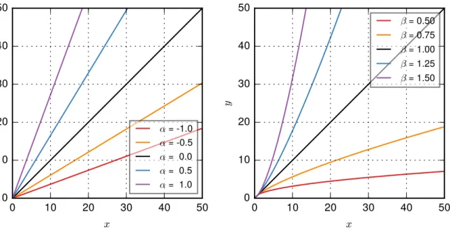
One way to visualize this is via Fig. A1, which shows the effects ofα andβ on linear axes for
447
xandy. α quantifies the “tilt” from the one-to-one line: with a perfectβ, the deterministic part of
448
the model becomesy=eαx, withα determining the gradient of the relationship. β characterizes
449
the departure from linearity: with a perfectα, the deterministic part of the model becomesy=xβ,
450
withβ being the exponent in the power-law relationship. With a logarithmic transformation, the
451
model becomes a straight line in log-log axes, withβ being the slope and α being the intercept
452
atx= 1. σ, on the other hand, quantifies the stochastic component in the model, representing the
453
spread of the points from the best fit curve ofy=eαxβ. As such, it can be considered as the spread
454
of the points after removing any systematic errors.
References
456
Bolvin, D. T., and G. J. Huffman, 2015: Transition of 3B42/3B43
Re-457
search Product from Monthly to Climatological Calibration/Adjustment.
458
https://pmm.nasa.gov/sites/default/files/document files/3B42 3B43 TMPA restart.pdf.
459
Chen, S., and Coauthors, 2013a: Evaluation and Uncertainty Estimation of NOAA/NSSL
Next-460
Generation National Mosaic Quantitative Precipitation Estimation Product (Q2) over the
Con-461
tinental United States.J. Hydrometeorol.,14 (4), 1308–1322, doi:10.1175/JHM-D-12-0150.1.
462
Chen, S., and Coauthors, 2013b: Similarity and difference of the two successive V6 and V7
463
TRMM multisatellite precipitation analysis performance over China. J. Geophys. Res.
Atmo-464
spheres,118 (23), 13,060–13,074, doi:10.1002/2013JD019964.
465
Ebert, E. E., J. E. Janowiak, and C. Kidd, 2007: Comparison of Near-Real-Time Precipitation
466
Estimates from Satellite Observations and Numerical Models.Bull. Am. Meteorol. Soc.,88 (1),
467
47–64, doi:10.1175/BAMS-88-1-47.
468
Falck, A. S., V. Maggioni, J. Tomasella, D. A. Vila, and F. L. Diniz, 2015: Propagation of satellite
469
precipitation uncertainties through a distributed hydrologic model: A case study in the
To-470
cantins–Araguaia basin in Brazil.J. Hydrol.,527, 943–957, doi:10.1016/j.jhydrol.2015.05.042.
471
Gebregiorgis, A., P.-E. Kirstetter, Y. Hong, N. Carr, J. J. Gourley, and Y. Zheng, 2016:
Under-472
standing Overland Multi-Sensor Satellite Precipitation Error in TRMM TMPA-RT Products.J.
473
Hydrometeorol., In Revision.
474
Gottschalck, J., J. Meng, M. Rodell, and P. Houser, 2005: Analysis of multiple precipitation
475
products and preliminary assessment of their impact on global land data assimilation system
476
land surface states.J. Hydrometeorol.,6 (5), 573–598, doi:10.1175/JHM437.1.
Gourley, J. J., Y. Hong, Z. L. Flamig, L. Li, and J. Wang, 2010: Intercomparison of Rainfall
478
Estimates from Radar, Satellite, Gauge, and Combinations for a Season of Record Rainfall.J.
479
Appl. Meteorol. Climatol.,49 (3), 437–452, doi:10.1175/2009JAMC2302.1.
480
Guo, H., S. Chen, A. Bao, A. Behrangi, Y. Hong, F. Ndayisaba, J. Hu, and P. M. Stepanian, 2016:
481
Early assessment of Integrated Multi-satellite Retrievals for Global Precipitation Measurement
482
over China.Atmospheric Res.,176-177, 121–133, doi:10.1016/j.atmosres.2016.02.020.
483
Habib, E., A. T. Haile, Y. Tian, and R. J. Joyce, 2012: Evaluation of the High-Resolution
484
CMORPH Satellite Rainfall Product Using Dense Rain Gauge Observations and Radar-Based
485
Estimates.J. Hydrometeorol.,13 (6), 1784–1798, doi:10.1175/JHM-D-12-017.1.
486
Habib, E., A. Henschke, and R. F. Adler, 2009: Evaluation of TMPA satellite-based research
487
and real-time rainfall estimates during six tropical-related heavy rainfall events over Louisiana,
488
USA.Atmospheric Res.,94 (3), 373–388, doi:10.1016/j.atmosres.2009.06.015.
489
Hong, Y., K.-L. Hsu, S. Sorooshian, and X. Gao, 2004: Precipitation estimation from remotely
490
sensed imagery using an artificial neural network cloud classification system.J. Appl. Meteorol.,
491
43 (12), 1834–1853.
492
Hossain, F., and G. J. Huffman, 2008: Investigating Error Metrics for Satellite Rainfall Data at
493
Hydrologically Relevant Scales.J. Hydrometeorol.,9 (3), 563–575, doi:10.1175/2007JHM925.
494
1.
495
Hou, A. Y., and Coauthors, 2014: The Global Precipitation Measurement Mission. Bull. Am.
496
Meteorol. Soc.,95 (5), 701–722, doi:10.1175/BAMS-D-13-00164.1.
Huffman, G. J., D. T. Bolvin, D. Braithwaite, K. Hsu, R. Joyce, C. Kidd, E. J. Nelkin, and P. Xie,
498
2015: Algorithm Theoretical Basis Document (ATBD) Version 4.5. NASA Global Precipitation
499
Measurement (GPM) Integrated Multi-satellitE Retrievals for GPM (IMERG). NASA.
500
Huffman, G. J., and Coauthors, 2007: The TRMM Multisatellite Precipitation Analysis (TMPA):
501
Quasi-Global, Multiyear, Combined-Sensor Precipitation Estimates at Fine Scales.J.
Hydrom-502
eteorol.,8 (1), 38–55, doi:10.1175/JHM560.1.
503
Joyce, R. J., J. E. Janowiak, P. A. Arkin, and P. Xie, 2004: CMORPH: A method that produces
504
global precipitation estimates from passive microwave and infrared data at high spatial and
tem-505
poral resolution. J. Hydrometeorol., 5 (3), 487–503, doi:10.1175/1525-7541(2004)005h0487:
506
CAMTPGi2.0.CO;2.
507
Joyce, R. J., and P. Xie, 2011: Kalman Filter–Based CMORPH.J. Hydrometeorol.,12 (6), 1547–
508
1563, doi:10.1175/JHM-D-11-022.1.
509
Kirstetter, P.-E., J. J. Gourley, Y. Hong, J. Zhang, S. Moazamigoodarzi, C. Langston, and
510
A. Arthur, 2015a: Probabilistic precipitation rate estimates with ground-based radar networks.
511
Water Resour. Res.,51, 1422–1442, doi:10.1002/2014WR015672.
512
Kirstetter, P.-E., Y. Hong, J. J. Gourley, Q. Cao, M. Schwaller, and W. Petersen, 2014: Research
513
Framework to Bridge from the Global Precipitation Measurement Mission Core Satellite to the
514
Constellation Sensors Using Ground-Radar-Based National Mosaic QPE. Geophysical
Mono-515
graph Series, V. Lakshmi, D. Alsdorf, M. Anderson, S. Biancamaria, M. Cosh, J. Entin, G.
Huff-516
man, W. Kustas, P. van Oevelen, T. Painter, J. Parajka, M. Rodell, and C. R¨udiger, Eds., John
517
Wiley & Sons, Inc, Hoboken, NJ, 61–79.
Kirstetter, P.-E., Y. Hong, J. J. Gourley, M. Schwaller, W. Petersen, and Q. Cao, 2015b: Impact
519
of sub-pixel rainfall variability on spaceborne precipitation estimation: Evaluating the TRMM
520
2A25 product: Impact of Sub-Pixel Rainfall Variability on TRMM 2A25. Q. J. R. Meteorol.
521
Soc.,141 (688), 953–966, doi:10.1002/qj.2416.
522
Kirstetter, P.-E., and Coauthors, 2012: Toward a Framework for Systematic Error Modeling
523
of Spaceborne Precipitation Radar with NOAA/NSSL Ground Radar–Based National Mosaic
524
QPE.J. Hydrometeorol.,13 (4), 1285–1300, doi:10.1175/JHM-D-11-0139.1.
525
Kubota, T., T. Ushio, S. Shige, S. Kida, M. Kachi, and K. ’ichi Okamoto, 2009: Verification
526
of High-Resolution Satellite-Based Rainfall Estimates around Japan Using a Gauge-Calibrated
527
Ground-Radar Dataset.J. Meteorol. Soc. Jpn.,87A, 203–222, doi:10.2151/jmsj.87A.203.
528
Liu, Z., 2016: Comparison of Integrated Multisatellite Retrievals for GPM (IMERG) and TRMM
529
Multisatellite Precipitation Analysis (TMPA) Monthly Precipitation Products: Initial Results.J.
530
Hydrometeorol.,17 (3), 777–790, doi:10.1175/JHM-D-15-0068.1.
531
Maggioni, V., M. R. P. Sapiano, R. F. Adler, Y. Tian, and G. J. Huffman, 2014: An Error Model for
532
Uncertainty Quantification in High-Time-Resolution Precipitation Products.J. Hydrometeorol.,
533
15 (3), 1274–1292, doi:10.1175/JHM-D-13-0112.1.
534
Mei, Y., E. N. Anagnostou, E. I. Nikolopoulos, and M. Borga, 2014: Error Analysis of Satellite
535
Precipitation Products in Mountainous Basins. J. Hydrometeorol., 15 (5), 1778–1793, doi:10.
536
1175/JHM-D-13-0194.1.
537
Roca, R., P. Chambon, I. Jobard, P.-E. Kirstetter, M. Gosset, and J. C. Berg`es, 2010: Comparing
538
Satellite and Surface Rainfall Products over West Africa at Meteorologically Relevant Scales
during the AMMA Campaign Using Error Estimates.J. Appl. Meteorol. Climatol.,49 (4), 715–
540
731, doi:10.1175/2009JAMC2318.1.
541
Sarachi, S., K.-l. Hsu, and S. Sorooshian, 2015: A Statistical Model for the Uncertainty
Anal-542
ysis of Satellite Precipitation Products. J. Hydrometeorol., 16 (5), 2101–2117, doi:10.1175/
543
JHM-D-15-0028.1.
544
Stampoulis, D., and E. N. Anagnostou, 2012: Evaluation of Global Satellite Rainfall Products
545
over Continental Europe.J. Hydrometeorol.,13 (2), 588–603, doi:10.1175/JHM-D-11-086.1.
546
Tan, J., W. A. Petersen, and A. Tokay, 2016: A Novel Approach to Identify Sources of Errors
547
in IMERG for GPM Ground Validation. J. Hydrometeorol., 17 (9), 2477–2491, doi:10.1175/
548
JHM-D-16-0079.1.
549
Tang, G., Y. Ma, D. Long, L. Zhong, and Y. Hong, 2016a: Evaluation of GPM Day-1 IMERG
550
and TMPA Version-7 legacy products over Mainland China at multiple spatiotemporal scales.
551
J. Hydrol.,533, 152–167, doi:10.1016/j.jhydrol.2015.12.008.
552
Tang, G., Z. Zeng, D. Long, X. Guo, B. Yong, W. Zhang, and Y. Hong, 2016b: Statistical and
Hy-553
drological Comparisons between TRMM and GPM Level-3 Products over a Midlatitude Basin:
554
Is Day-1 IMERG a Good Successor for TMPA 3B42V7? J. Hydrometeorol., 17 (1), 121–137,
555
doi:10.1175/JHM-D-15-0059.1.
556
Tang, L., Y. Tian, F. Yan, and E. Habib, 2015: An improved procedure for the validation of
557
satellite-based precipitation estimates. Atmospheric Res., 163, 61–73, doi:10.1016/j.atmosres.
558
2014.12.016.
Tian, Y., G. J. Huffman, R. F. Adler, L. Tang, M. Sapiano, V. Maggioni, and H. Wu, 2013:
Model-560
ing errors in daily precipitation measurements: Additive or multiplicative? Geophys. Res. Lett.,
561
40 (10), 2060–2065, doi:10.1002/grl.50320.
562
Tian, Y., G. S. Nearing, C. D. Peters-Lidard, K. W. Harrison, and L. Tang, 2016: Performance
563
Metrics, Error Modeling, and Uncertainty Quantification. Mon. Weather Rev., 144 (2), 607–
564
613, doi:10.1175/MWR-D-15-0087.1.
565
Tian, Y., and C. D. Peters-Lidard, 2007: Systematic anomalies over inland water bodies in
566
satellite-based precipitation estimates. Geophys. Res. Lett., 34 (14), L14 403, doi:10.1029/
567
2007GL030787.
568
Tian, Y., C. D. Peters-Lidard, B. J. Choudhury, and M. Garcia, 2007: Multitemporal Analysis
569
of TRMM-Based Satellite Precipitation Products for Land Data Assimilation Applications. J.
570
Hydrometeorol.,8 (6), 1165–1183, doi:10.1175/2007JHM859.1.
571
Wilks, D. S., 2011: Statistical Methods in the Atmospheric Sciences. 3rd ed., No. 100,
Interna-572
tional geophysics series, Elsevier/Acad. Press, Amsterdam.
573
Xue, X., Y. Hong, A. S. Limaye, J. J. Gourley, G. J. Huffman, S. I. Khan, C. Dorji, and
574
S. Chen, 2013: Statistical and hydrological evaluation of TRMM-based Multi-satellite
Pre-575
cipitation Analysis over the Wangchu Basin of Bhutan: Are the latest satellite
precipita-576
tion products 3B42V7 ready for use in ungauged basins? J. Hydrol., 499, 91–99, doi:
577
10.1016/j.jhydrol.2013.06.042.
578
Zhang, J., Y. Qi, K. Howard, C. Langston, and B. Kaney, 2011a: Radar quality index (RQI)—A
579
combined measure of beam blockage and VPR effects in a national network.Proc. Eighth Int.
580
Symp. on Weather Radar and Hydrology, 388–393.
Zhang, J., and Coauthors, 2011b: National Mosaic and Multi-Sensor QPE (NMQ) System:
582
Description, Results, and Future Plans. Bull. Am. Meteorol. Soc., 92 (10), 1321–1338, doi:
583
10.1175/2011BAMS-D-11-00047.1.
LIST OF FIGURES
585
Fig. 1. A map of the average RQI for 2015. The red box shows our region of analysis: 30.0–41.5◦N, 586
93.5–83.5◦W. . . 30
587
Fig. 2. A scatter diagram between IMERG and the reference at different scales: (a) 0.1◦×0.1◦grid 588
box at 0.5 h, (b) 0.1◦×0.1◦grid box at 24 h, (c) 2.5◦×2.5◦grid box at 0.5 h, and (d) 2.5◦ 589
×2.5◦grid box at 24 h. . . 31
590
Fig. 3. Fraction of occurrences for which the reference is at least 0.2 mm / h. These fractions are 591
obtained by sampling different spatial and temporal scales a hundred times. . . 32 592
Fig. 4. Thresholds for raining events as a function of scale. Solid lines are for IMERG comparisons 593
while dashed lines are for TMPA comparisons. . . 33
594
Fig. 5. Hits, misses, false alarms and correct rejections in IMERG (solid lines) and in TMPA 595
(dashed lines) as a function of scale. . . 34
596
Fig. 6. Probability of detection, false alarm ratio, bias in detection, and Heidke skill score of 597
IMERG (solid lines) and of TMPA (dashed lines) as a function of scale. . . 35
598
Fig. 7. Correlations of the hits between IMERG and the reference (solid lines), and TMPA and the 599
reference (dashed lines) as a function of scale. . . 36
600
Fig. 8. Normalized mean errors, normalized mean absolute errors and normalized root-mean-square 601
errors (RMSE) of the hits in IMERG (solid lines) and in TMPA (dashed lines) as a function 602
of scale. . . 37
603
Fig. 9. Multiplicative error model parameters of the hits in IMERG (solid lines) and in TMPA 604
(dashed lines) as a function of scale. . . 38
605
Fig. A1. The effects ofα withβ = 1 (left) andβ withα = 0 (right) from the multiplicative error 606
model on a linear axes. . . 39
30°N 41.5°N 93.5°W 83.5°W 20°N 40°N 60°N 130°W 110°W 90°W 70°W 0 10 20 30 40 50 60 70 80 90 100
FIG. 1. A map of the average RQI for 2015. The red box shows our region of analysis: 30.0–41.5◦N, 93.5– 83.5◦W.
608 609
10-1 100 101 102 10-1 100 101 102 IMERG (mm / h) (a) 0.1°, 0.5 h 10-1 100 101 102 10-1 100 101 102 (b) 0.1°, 24 h 10-1 100 101 102 reference (mm / h) 10-1 100 101 102 IMERG (mm / h) (c) 2.5°, 0.5 h 10-1 100 101 102 reference (mm / h) 10-1 100 101 102 (d) 2.5°, 24 h
FIG. 2. A scatter diagram between IMERG and the reference at different scales: (a) 0.1◦×0.1◦grid box at 0.5 h, (b) 0.1◦×0.1◦grid box at 24 h, (c) 2.5◦×2.5◦grid box at 0.5 h, and (d) 2.5◦×2.5◦grid box at 24 h. 610
0.0 0.5 1.0 1.5 2.0 2.5 box length (°)
0.10 0.15 0.20
fraction of events with at least 0.2 mm / h
0.5 h 1 h 3 h 6 h 12 h 24 h
FIG. 3. Fraction of occurrences for which the reference is at least 0.2 mm / h. These fractions are obtained by sampling different spatial and temporal scales a hundred times.
612 613
0.0 0.5 1.0 1.5 2.0 2.5 box length (°) 0.00 0.05 0.10 0.15 0.20 0.25 threshold (mm / h) 0.5 h 1 h 3 h 6 h 12 h 24 h
FIG. 4. Thresholds for raining events as a function of scale. Solid lines are for IMERG comparisons while dashed lines are for TMPA comparisons.
614 615
0 10 20 30 40 50 60 hit (%) 3 4 5 6 7 8 9 10 11 12 miss (%) 0.5 h 1 h 3 h 6 h 12 h 24 h 0.0 0.5 1.0 1.5 2.0 2.5 box length (°) 2 4 6 8 10 12 14 16 false alarm (%) 0.0 0.5 1.0 1.5 2.0 2.5 box length (°) 20 30 40 50 60 70 80 90 100 correct rejection (%)
FIG. 5. Hits, misses, false alarms and correct rejections in IMERG (solid lines) and in TMPA (dashed lines) as a function of scale.
616 617
0.50 0.55 0.60 0.65 0.70 0.75 0.80 0.85 0.90 probability of detection 0.05 0.10 0.15 0.20 0.25 0.30 0.35 0.40 0.45
false alarm ratio
0.5 h 1 h 3 h 6 h 12 h 24 h 0.0 0.5 1.0 1.5 2.0 2.5 box length (°) 0.80 0.85 0.90 0.95 1.00 1.05 1.10 1.15 bias in detection 0.0 0.5 1.0 1.5 2.0 2.5 box length (°) 0.45 0.50 0.55 0.60 0.65 0.70
Heidke skill score
FIG. 6. Probability of detection, false alarm ratio, bias in detection, and Heidke skill score of IMERG (solid lines) and of TMPA (dashed lines) as a function of scale.
618 619
0.0 0.5 1.0 1.5 2.0 2.5 box length (°) 0.3 0.4 0.5 0.6 0.7 0.8 0.9 correlation 0.5 h 1 h 3 h 6 h 12 h 24 h
FIG. 7. Correlations of the hits between IMERG and the reference (solid lines), and TMPA and the reference (dashed lines) as a function of scale.
620 621
−0.10 −0.05 0.00 0.05 0.10 0.15
norm. mean error
0.4 0.5 0.6 0.7 0.8 0.9 1.0
norm. mean abs. error
0.5 h 1 h 3 h 6 h 12 h 24 h 0.0 0.5 1.0 1.5 2.0 2.5 box length (°) 0.8 1.0 1.2 1.4 1.6 1.8 norm. RMSE
FIG. 8. Normalized mean errors, normalized mean absolute errors and normalized root-mean-square errors (RMSE) of the hits in IMERG (solid lines) and in TMPA (dashed lines) as a function of scale.
622 623
−0.8 −0.6 −0.4 −0.2 0.0 0.2 0.4 ® 0.5 h 1 h 3 h 6 h 12 h 24 h 0.4 0.5 0.6 0.7 0.8 0.9 1.0 1.1 ¯ 0.0 0.5 1.0 1.5 2.0 2.5 box length (°) 0.95 1.00 1.05 1.10 1.15 1.20 1.25 1.30 ¾
FIG. 9. Multiplicative error model parameters of the hits in IMERG (solid lines) and in TMPA (dashed lines) as a function of scale.
624 625
0 10 20 30 40 50 x 0 10 20 30 40 50 y ® = -1.0 ® = -0.5 ® = 0.0 ® = 0.5 ® = 1.0 0 10 20 30 40 50 x 0 10 20 30 40 50 y ¯ = 0.50 ¯ = 0.75 ¯ = 1.00 ¯ = 1.25 ¯ = 1.50
Fig. A1. The effects ofαwithβ = 1 (left) andβ withα= 0 (right) from the multiplicative error model on a
linear axes. 626