Avoiding Liquidity Traps

(1)

ECONOMIC RESEARCH REPORTS

C.V. STARR CENTER

FOR APPLIED ECONOMICS

NEW YORK UNIVERSITY

FACULTY OF ARTS AND SCIENCE

DEPARTMENT OF ECONOMICS

WASHINGTON SQUARE

NEW YORK, NY 10003-6687

Avoiding Liquidity Traps

By

Jess Benhabib,

Stephanie Schmitt-Grohe,

&

Martin Uribe

RR# 99-21

December 1999

(2)

Avoiding Liquidity Traps

∗

Jess Benhabib

†

New York University

Stephanie Schmitt-Groh´

e

‡

Rutgers University and CEPR

Mart´ın Uribe

§

University of Pennsylvania

January 1, 2000

Abstract

Once the zero bound on nominal interest rates is taken into account, Taylor-type interest-rate feedback rules give rise to unintended self-fulfilling decelerating inflation paths and aggregate fluctuations driven by arbitrary revisions in expectations. These undesirable equilibria exhibit the essential features of liquidity traps, as monetary pol-icy is ineffective in bringing about the government’s goals regarding the stability of output and prices. This paper proposes several fiscal and monetary policies that pre-serve the appealing features of Taylor rules, such as local uniqueness of equilibrium near the inflation target, and at the same time rule out the deflationary expectations that can lead an economy into a liquidity trap.

JELClassiﬁcation Numbers: E52, E31, E63.

Keywords: Taylor rules, liquidity traps, zero bound on nominal interest rates.

∗_{We thank the C.V. Starr Center of Applied Economics at New York University for technical assistance.} †_{Phone: 212 998-8066. Email: [email protected].}

‡_{Phone: 732 932 2960. Email: [email protected].} §_{Phone: 215 898 6260. Email: [email protected].}

(3)

1

Introduction

In recent years, there has been a revival of empirical and theoretical research aimed at understanding the macroeconomic consequences of monetary policy regimes that take the form of interest-rate feedback rules. One driving force of this renewed interest can be found in empirical studies showing that in the past two decades monetary policy in the United States is well described as following such a rule. In particular, an influential paper by Taylor (1993) characterizes the Federal Reserve as following a simple rule whereby the federal funds rate is set as a linear function of inflation and the output gap with coefficients of 1.5 and 0.5, respectively. Taylor emphasizes the stabilizing role of an inflation coefficient greater than unity, which loosely speaking implies that the central bank raises real interest rates in response to increases in the rate of inflation. After his seminal paper, interest-rate feedback rules with this feature have become known as Taylor rules. Taylor rules have also been shown to represent an adequate description of monetary policy in other industrialized economies (see, for example, Clarida, Gal´ı, and Gertler, 1998).

At the same time, a growing body of theoretical work has argued that Taylor rules contribute to macroeconomic stability. Researchers have arrived at this conclusion following different routes. For example, Levin, Wieland, and Williams (1999) use a non-optimizing, rational expectations model and find that a Taylor rule is the optimal interest-rate feedback rule in the sense that it minimizes a quadratic loss function of inflation and output deviations from their respective target levels. Rotemberg and Woodford (1999) find a similar result using a dynamic, optimizing, general equilibrium model and a welfare criterion for policy evaluation. Leeper (1991), Bernanke and Woodford (1997), and Clarida, Gal´ı, and Gertler (1997) argue that Taylor rules contribute to aggregate stability because they guarantee the uniqueness of the rational expectations equilibrium whereas interest rate feedback rules with an inflation coefficient of less than unity, also referred to as passive rules, are destabilizing because they render the equilibrium indeterminate, thus allowing for expectations-driven fluctuations.

(4)

Two important elements are common across these methodologically diverse studies: first, they restrict attention to local dynamics, or small fluctuations, around a target level of inflation; and second, they do not take into account the fact that nominal interest rates are bounded below by zero. These two simplifications have serious consequences for aggregate stability. In Benhabib, Schmitt-Grohé and Uribe (2000), we show, in the context of dynamic, optimizing, general equilibrium models, with and without nominal rigidities, that if the zero bound on nominal rates is taken into account and global dynamics are characterized, then Taylor rules may in fact lose their appealing stability properties. In particular, equilibria emerge in which inflation and the nominal interest rate start arbitrarily close to the intended targets and converge gradually to a different long-run equilibrium in which both variables are below target and monetary policy is passive. Moreover, this unintended long-run equilibrium fails to be locally unique. For in its neighborhood stationary sunspot equilibria exist in which inflation, interest rates, and aggregate activity fluctuate in response to non-fundamental revisions in expectations.1

When the economy falls into this type of decelerating inflation dynamics, it is headed to a situation of low and possibly negative inflation and low and possibly zero interest rates in which monetary policy becomes ineffective in bringing about the government’s goals regarding the stability of output and prices. This state of matters has all the essential characteristics of a liquidity trap, at the heart of which there is a central bank that is powerless to reverse the downward slide in prices through expansionary monetary policy in the form of lower and lower interest rates.

The central focus of this paper is the design of ﬁscal and monetary policies that preserve the Taylor rule, and with it all its desirable local properties, around the target rate of inﬂation and real activity, and at the same time eliminate equilibrium dynamics leading to the liquidity trap.

1_{A branch of the literature has focused on the limitations that the zero bound on nominal interest rates}

imposes on the government’s ability to conduct countercyclical monetary policy. Model-based assessments of the costs associated with these limitations are contained in Fuhrer and Madigan (1997), Orphanides and Wieland (1998), Reifschneider and Williams (1999), and Wolman (1999).

(5)

Two broad approaches to avoiding liquidity traps are presented. In the first one, liquidity traps are ruled out by means of fiscal policy while maintaining the assumption that monetary policy follows everywhere an interest-rate rule. The proposed stabilization policy features a strong fiscal stimulus that is automatically activated when inflation begins to decelerate. Specifically, the fiscal rule consists of an inflation sensitive budget surplus schedule that calls for lowering taxes when inflation subsides. As the economy approaches the liquidity trap, fiscal deficits become large enough so that this low-inflation steady state becomes fiscally unsustainable and ceases to be a rational expectations equilibrium.

This result thus provides theoretical support for the recent policy proposals—emanating most notably from the U.S. Department of Treasury—suggesting that economies with near-zero nominal interest rates and thus little room for monetary stabilization policy, such as Japan, should spend their way out of the liquidity trap.2 However, we arrive at this policy recommendation for very different reasons. The fiscal stimulus eliminates the liquidity trap not through the traditional Keynesian multiplier, as is the conventional wisdom, but rather by affecting the intertemporal budget constraint of the government. The channel thorough which the liquidity trap is eliminated here is more akin to Pigou’s argument on the implau-sibility of liquidity traps. In a closed economy, the intertemporal budget constraint of the government is the mirror image of the intertemporal budget constraint of the representative household. A decline in taxes increases the household’s after-tax wealth, which induces an aggregate excess demand for goods. As a consequence the price level must increase in order to re-establish equilibrium in the goods market.

The second approach consists of switching from an interest rate rule to a money growth rate peg should inflation embark on a self-fulfilling decelerating path. This alternative is a popular one, frequently mentioned in the policy debate: when caught in a low inflation equilibrium, governments should simply start printing money to jump start the economy.

2_{See, for example, the June 24, 1998 testimony of Lawrence Summers, then deputy secretary of the}

Treasury, before a Senate Foreign Aﬀairs subcommittee and his remarks to the World Economic Development Congress held on October 1, 1998 in Washington, DC.

(6)

Krugman (1998), for example, argues forcefully for this type of policy as a way to bring Japan out of its current recession. However, this recommendation is typically made without any reference to the accompanying fiscal policy. An important result of this paper is that switching to a money growth rate rule is a successful tool to avoid or escape a liquidity trap only if coupled with the “right” fiscal policy. For instance, if the fiscal regime in place at the time of the switch to a money growth rule is one that guarantees fiscal sustainability under all circumstances, then printing money may in fact be counterproductive as it is likely to accelerate the deflationary spiral. In general, what is needed to make the switch to a money growth rate rule successful is a fiscal policy that, as nominal interest rates approach zero, makes the government intertemporally insolvent.

The remainder of the paper is organized in five sections. Section 2 presents the model and the baseline monetary-fiscal regime. Section 3 shows how the economy can fall into a liquidity trap when monetary policy takes the form of a Taylor-type interest-rate feedback rule. Sections 4 and 5 develop, respectively, fiscal and monetary instruments capable of eliminating liquidity traps. Section 6 closes the paper by discussing the robustness of the results to important model perturbations such as the introduction of nominal frictions, the treatment of time as discrete, and the inclusion of Gesell taxes, which have been suggested in the related literature as a possible way to avoid liquidity traps.

2

The model

In this section we use a simple economic environment to illustrate how a monetary–fiscal regime frequently advocated on the basis of aggregate stability can in fact lead to expecta-tional traps. The difference between our analysis and that found in the related literature is twofold: first, we do not restrict the analysis to local dynamics around a particular station-ary state. Second, we take explicit account of the zero bound on nominal interest rates in the specification of interest rate feedback rules.

(7)

2.1

Households

Consider an endowment economy populated by a large number of identical inﬁnitely lived households with preferences deﬁned over consumption and real balances and described by the utility function

_∞

0

e−rtu(c, M/P)dt, (1)

wherecdenotes consumption, M denotes nominal money balances, andP denotes the price level. The instantaneous utility index u is assumed to be increasing in both arguments, concave, and to satisfy ucm > 0, so that consumption and real balances are Edgeworth

complements, and limm→∞ u_um(_c(_y,my,m₎) = 0∀y >0, which implies that money demand approaches

inﬁnity as the nominal interest rate vanishes. In addition to ﬁat money, the representative household has access to nominal government bonds, denoted by B, that pay the nominal interest rateR. The household is endowed with a constant stream of perishable goodsy and pays real lump-sum taxes τ. Its instant budget constraint is then given by

P c+P τ + ˙M + ˙B =RB+P y.

Lettingm≡M/P denote real balances anda ≡(M+B)/P real ﬁnancial wealth, the above constraint can be written as

c+τ + ˙a= (R−π)a−Rm+y, (2)

where π ≡ P /P˙ denotes the instant rate of inﬂation. The right-hand side of this budget constraint represents the sources of income: real interest on the household’s assets net of the opportunity cost of holding money and the endowment. The left hand side shows the uses of income: consumption, tax payments, and savings. Households are also subject to a

(8)

borrowing limit of the form

lim

t→∞e

−R₀t[R(s)−π(s)]ds_a₍_t₎_≥₀ ₍₃₎

that prevents them from engaging in Ponzi games. This no-Ponzi-game constraint says that the household is not permitted to implement consumption and money-holding plans that imply that its real debt position net of money holdings grows at a rate higher than or equal to the real interest rate. Clearly, because the utility function is increasing in consumption and real balances, the household will always ﬁnd it optimal to satisfy the above borrowing limit with equality. The representative household chooses paths for consumption, real balances, and wealth so as to maximize (1) subject to the instant budget constraint (2) and the borrowing limit (3), given its initial real wealth, a(0), and the paths of taxes, inﬂation, and nominal interest rates. The associated optimality conditions are (2), (3) holding with equality, and

uc(c, m) =λ (4)

um(c, m) =λR (5)

˙

λ=λ[r+π−R], (6)

where λ is a Lagrange multiplier associated with the instant budget constraint.

2.2

Monetary and ﬁscal policy

We assume that the monetary authority follows an interest-rate feedback rule of the form

R =R(π). (7)

We refer to monetary policy as active at an inﬂation rate π if R(π) > 1 and as passive if

(9)

interest rate in response to an increase in inﬂation and is passive if the central bank fails to do so.

Three assumptions regarding the form of this feedback rule are of great consequence for the subsequent results: ﬁrst, we assume that the nominal interest rate is non-decreasing in inﬂation, that is,

R(π)≥0 ∀π.

Second, the interest rate feedback rule satisﬁes the zero bound on nominal interest rates in that regardless of how low the inﬂation rate may be, the monetary authority will never threaten to implement a negative nominal rate. Thus,

R(π)≥0 ∀π.

Third, we assume that the central bank targets a rate of inflation π∗ > −r and that, in the spirit of Taylor (1993), it conducts an active monetary policy around its inflation target by responding to increases (decreases) in inflation with a more than one-for-one increase (decrease) in the nominal interest rate. Formally,

∃ π∗ >−r : R(π∗) =r+π∗ and R(π∗)>1. (8) The government ﬁnances its deﬁcits by printing money, M, and issuing nominal bonds,

B, that pay the nominal interest rateR. We assume that public consumption is zero and that the government levies real lump-sum taxes, τ. Therefore, the sequential budget constraint of the government is given by ˙B =RB−M˙ −P τ, which can be written as

˙

(10)

By deﬁnition, the initial condition a(0) satisﬁes

a(0) = A(0)

P(0), (10)

where A(0) ≡ M(0) +B(0) > 0 denotes the initial level of total nominal government lia-bilities. Following Benhabib, Schmitt-Grohé, and Uribe (1999), we classify fiscal policies as either Ricardian or Non-Ricardian. Ricardian fiscal policies are those that ensure that the present discounted value of total government liabilities converges to zero—that is,

lim

t→∞e

−R₀t[R(s)−π(s)]ds_a₍_t_{) = 0} ₍₁₁₎

is satisfied under all possible, equilibrium or off-equilibrium, paths of endogenous variables, such as the price level, the money supply, inflation, or the nominal interest rate. In this section, we restrict attention to one particular Ricardian fiscal policy that takes the form

τ +Rm=α a, (12)

where the sequence α is chosen arbitrarily by the government subject to the constraint that it is positive and bounded below by some α > 0. This policy states that consolidated government revenues, that is, tax revenues plus interest savings from the issuance of money, are always higher than a certain fraction α of total government liabilities. A special case of this type of policy is a balanced-budget rule whereby tax revenues are equal to interest payments on the debt, which results when α = R, provided R is bounded away from zero (Benhabib, Schmitt-Groh´e, and Uribe, 1999).

(11)

2.3

Equilibrium

Equilibrium in the goods market requires that consumption be equal to the endowment

c=y. (13)

Given the assumptions regarding the form of the instant utility function, equations (4), (5), and (13) deﬁne a decreasing function linking λ and R:

λ=L(R); L <0. (14)

Combining the feedback rule (7) with (4) and (14), we obtain the following ﬁrst-order dif-ferential equation describing the equilibrium dynamics of inﬂation

R(π) ˙π= −L(R(π))

L(R(π)) [R(π)−π−r]. (15)

In turn, combining the government budget constraint (9) with the monetary and ﬁscal policy rules, equations (7) and (12), yields

˙

a = (R(π)−π−α)a (16)

Finally, using (7) to eliminate R from (11), the transversality condition becomes

lim

t→∞e

−R₀t[R(π(s))−π(s)]ds_a₍_t_{) = 0} ₍₁₇₎

A perfect-foresight competitive equilibrium is defined as an initial price levelP(0) and func-tions of time π and a satisfying (10) and (15)-(17), given the initial condition A(0). Note that because of the assumed Ricardian nature of the fiscal policy regime, given a function π, equations (10) and (16) imply a path for athat satisfies the transversality condition for any initial price level P(0) > 0. It follows immediately that if an equilibrium exists, then the

(12)

initial price level is indeterminate. However, this nominal indeterminacy is not the focus of

our analysis. We are instead concerned with real determinacy, that is, the determinacy of

the function π, which in turn governs the determination of real balances and thus welfare.

3

Falling into liquidity traps

Consider ﬁrst the steady-state solutions to equation (15), that is, constant inﬂation rates satisfying

R(π) =r+π.

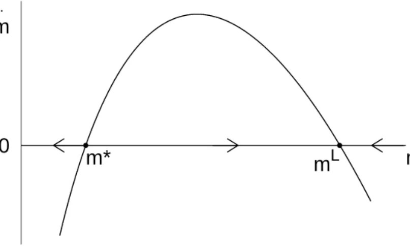
By the assumption given in (8), π∗ represents a steady-state inﬂation rate. Because π is a non-predetermined variable, π∗ is, in fact, a perfect-foresight equilibrium. But π∗ is not the only equilibrium. To see this, note that the existence of a steady state at which monetary policy is active together with the assumptions that the interest-rate feedback rule is non-decreasing and non-negative imply the existence of an inﬂation rate πL < π∗ satisfying

R(πL) = r+πL. To facilitate the analysis, we assume that R(π) is smooth and strictly increasing and that R(πL₎_>_{0. The case that} _R₍_πL_{) = 0 is treated in the appendix, where}

we show that the results of this section also obtain in this case. Clearly, πL _represents

a steady-state equilibrium. This second steady-state equilibrium has the properties that monetary policy is passive and that the inﬂation rate is below the target inﬂation rate.3 Figure 1 illustrates the multiplicity of steady-state equilibria.

Consider now the existence of equilibria other than the steady states. Note that, because

−L/(LR) is always positive, the sign of ˙π in equation (15) is the same as the sign of

R(π)−π−r. Because R(π∗)>1, it follows that the high-inﬂation, active steady state π∗

3_{In the context of the present ﬂexible-price, endowment economy, the low-inﬂation steady-state}

equilib-rium πL is in fact preferred to the target steady-state equilibriumπ∗ for it is associated with higher real balances and thus higher levels of utility. However, as shown in Benhabib, Schmitt-Groh´e, and Uribe (2000), in the presence of nominal rigidities, the low inﬂation equilibrium may be welfare inferior to the target steady state.

(13)

Figure 1: The liquidity trap in a ﬂexible price model

π

*

π

L

π

⋅

<0

π

⋅

>0

π

>0

⋅

r+

π

R(

π

)

is unstable, in the sense that trajectories initiating near π∗ diverge from π∗. Thus, if one limits the analysis to equilibria in which π remains forever in a small neighborhood around

π∗, then the only perfect-foresight equilibrium is the active steady state itself. This local uniqueness result has served as one key theoretical argument for advocating the use of active, or Taylor-type, interest-rate feedback rules to ensure aggregate stability (e.g., Leeper, 1991; and Clarida, Gal´ı, and Gertler, 1997).

The local equilibrium dynamics in the neighborhood of the low-inﬂation steady state πL

are quite diﬀerent from those around the target steady stateπ∗. SinceR(πL₎_<_{1, it follows}

that ˙π is decreasing inπ for πnear πL_{. This implies that inﬂation trajectories originating in}

the vicinity of πL converge to πL and thus can be supported as perfect-foresight equilibria. Therefore, the low-inﬂation steady state is not locally unique. The local indeterminacy of equilibrium around πL gives rise to aggregate instability in the form of stationary sunspot equilibria.4

4_{For a general result on the existence of stationary sunspot equilibria in continuous-time models displaying}

(14)

In addition, as is evident from ﬁgure 1, there exists a large number of equilibrium tra-jectories originating arbitrarily close to (and to the left of) π∗ that converge smoothly and monotonically to πL_{. Along such paths the central bank, following the prescription of the}

Taylor rule, continuously eases in an attempt to reverse the persistent decline in inflation. But these efforts are in vain, and indeed counterproductive, for they introduce further down-ward pressure on inflation. This state of matters, in which monetary policy fails to stop the deceleration in prices, is central to the notion of a liquidity trap. Another aspect of these dynamics that is essential to the concept of liquidity traps is their self-fulfilling nature: all that is needed to fall into the liquidity trap is that people expect the economy to slide into a phase of decelerating inflation.

4

Avoiding liquidity traps through ﬁscal policy

In this section, we develop policy schemes designed to eliminate the liquidity trap. The strategy is to modify fiscal policy while maintaining the assumed monetary policy. Specifi-cally, we consider fiscal adjustment mechanisms that are automatically activated whenever the economy embarks on a self-fulfilling path of decelerating inflation. These mechanisms will rule out liquidity traps by making the low-inflation steady state fiscally unsustainable.

4.1

An inﬂation-sensitive revenue schedule

Consider replacing the Ricardian ﬁscal policy given by (12) with one in which the coeﬃcient

α, reflecting the sensitivity of consolidated government revenues with respect to the level of total government liabilities, is an increasing function of the inflation rate. Specifically, the fiscal policy now takes the form

(15)

We impose the following additional restrictions on the function α:

α(π∗)>0 (19)

and

α(πL)<0. (20)

This policy guarantees that the intended steady state π∗ is a perfect-foresight equilibrium and at the same time rules out the liquidity trapπL _{as an equilibrium outcome. To see this,}

combine (18) and the Taylor rule (7) with the instant government budget constraint (9) to obtain the following equilibrium law of motion fora:

˙

a= (R(π)−π−α(π))a. (21)

Solving this diﬀerential equation one obtains,

a(t) =eR0t(R(π(s))−π(s)−α(π(s)))ds_a₍₀₎_,

which implies that

lim

t→∞e

−R₀t[R(s)−π(s)]ds_a₍_t_{) =}_a_{(0) lim} t→∞e

−R₀tα(π(s))ds ₍₂₂₎

Consider an inﬂation trajectory along which π =π∗. By condition (19), the right hand side of (22) equals zero. Therefore, the transversality condition is satisﬁed andπ =π∗ represents a perfect-foresight equilibrium.

On the other hand, for an inﬂation trajectory in which π converges to the liquidity trap

πL_{, condition (20) implies that the right hand side of (22) does not converge to zero (except}

(16)

zero), thus violating the transversality condition. As a result, no inﬂation path leading to the liquidity trap can be supported as an equilibrium outcome.

Targeting the growth rate of nominal government liabilities

Consider a ﬁscal policy rule consisting in pegging the growth rate of total nominal government liabilities. That is,

˙

A

A =k, (23)

where k is assumed to satisfy

R(πL)< k < R(π∗). (24)

Expressing ˙A/A as ˙a/a +π and combining the above ﬁscal policy rule with the instant government budget constraint (9) yields

τ +Rm= [R(π)−k]a.

This fiscal policy rule is a special case of the one given in equation (18) whenα(π) takes the form R(π)−k. In particular, note that, because the Taylor rule is increasing in the rate of inflation, so isR(π)−k. Furthermore, condition (24) implies that restrictions (19) and (20) are satisfied. It follows immediately that targeting the growth rate of nominal government liabilities is a potential way of eliminating equilibrium deflationary spirals.

Under this policy, the government manages to fend off a low inflation equilibrium by threatening to implement a fiscal stimulus package consisting in a severe increase in the consolidated deficit should the inflation rate become sufficiently low. Interestingly, this type of policy prescription is what the U.S. Treasury as well as a large number of academic and professional economists are advocating as a way for Japan to lift itself out of its current

(17)

deﬂationary trap.

Abalanced-budget requirement

Consider now a ﬁscal policy rule consisting of a zero secondary deﬁcit, that is,

P τ =RB,

whereB denotes outstanding interest-bearing public debt. This policy rule requires that the government equates its primary surplus, P τ, to interest payments on the public debt, RB, so that the secondary deﬁcit, given by RB −P τ, is always equal to zero. Recalling that

a=B/P +m, we can rewrite the balanced-budget rule as

τ +Rm=R(π)a.

It follows that a balanced-budget requirement is a special case of the fiscal policy rule given in (21) in which α(π) = R(π). Clearly, in this case α(π) is increasing because so is R(π). Condition (19) is satisfied because R(π∗) is by assumption greater than zero. On the other hand, condition (20) is not satisfied because of our maintained assumption that

R(πL₎_>_{0. However, if one relaxes this assumption by considering the case of a Taylor rule}

that stipulates zero nominal interest rates at suﬃciently low rates of inﬂation, it becomes clear that a balanced-budget rule eliminates the liquidity trap as long as nominal interest rate paths leading to the liquidity trap satisfy limt→∞

t

0 R(s)ds < ∞. To see why, note

that under a balanced-budget rule the law of motion of real total government liabilities is given by ˙a =−πa. Combining this expression with the transversality condition (11) yields limt→∞a(0)e−

R_t

0R(s)ds = 0. In the appendix, we present two examples involving a Taylor rule that sets the nominal interest rate to zero at low rates of inﬂation. In one of the examples paths leading to the liquidity trap feature nominal interest rates that converge to zero but never actually reach that ﬂoor. In the other example, the nominal interest rate reaches the

(18)

zero bound in finite time. We show that in both cases, a balanced-budget rule succeeds in averting the liquidity trap. These examples show that it is in principle possible to escape the liquidity trap without generating fiscal deficits, if the central bank is credibly committed to conducting unlimited open market operations at zero nominal interest rates in the event that inflation falls below a certain threshold.

5

Avoiding liquidity traps through a monetary-regime

switch

Thus far, we have studied the design of fiscal policies capable of eliminating liquidity traps when the monetary authority follows an interest-rate feedback rule that is valid globally (i.e., for all possible values of the inflation rate). An alternative route to avoiding self-fulfilling liquidity traps is to modify monetary policy when the economy seems to be headed toward a low-inflation spiral. For example, in the case of Japan, a frequently advocated strategy to lift the economy out of deflation is for the Bank of Japan to switch to a money growth rate target letting interest rates be market determined. In this section, we show that abandoning an interest rate feedback rule in favor of a monetary target when inflation reaches dangerously low levels can be a successful way to avoid falling into a deflationary trap, but it need not be. The effectiveness of such alternative will in general depend upon the accompanying fiscal regime. We illustrate this general conclusion by means of two examples.

5.1

Switching to a money growth rule is ineﬀective when ﬁscal

policy is Ricardian

We begin by showing that under the Ricardian fiscal policy rule given by (12), switching from an interest-rate feedback rule to a money growth rate rule as the nominal interest rate gets close to zero will not eliminate self-fulfilling deflations. To establish this result, it

(19)

is enough to show that under this fiscal regime self-fulfilling deflations exist even under a money growth rate rule. Specifically, assume that monetary policy takes the form

˙

M

M =µ, (25)

where µ >−r is a constant.5 This monetary policy implies that

˙

m

m =µ−π. (26)

A perfect-foresight equilibrium can then be deﬁned as functions of time c, m, π, λ, and

R satisfying (4), (5), (6), (13) and (26). As we have shown above, under the assumed fiscal policy the transversality condition (17) is always satisfied, so we do not include it in our definition of equilibrium. Combining the equilibrium conditions yields the following differential equation in real balances:

˙ m= r+µ− um(y,m) uc(y,m) 1 m + ucm(y,m) uc(y,m) . (27)

Any functionmsatisfying this diﬀerential equation represents a perfect-foresight equilibrium. Figure 2 depicts the corresponding phase diagram. Becausemis a jump variable, one possible equilibrium is a steady-state equilibrium given by m=m, where m is a constant satisfying

r+µ= um(y,m)

uc(y,m)

.

Given our maintained assumptions that consumption and real balances are Edgeworth com-plements (ucm > 0) and that the instant utility index is concave (so that umm < 0), we

have that there is a unique steady-state equilibrium and that ˙m >0 for m >m and ˙m <0

5_{Note that we allow for both positive and negative rates of monetary expansion. This is of interest for}

the results that follow because under the fiscal regime typically assumed in the literature on speculative deflations (namely, B= 0 at all times), self-fulfilling deflations occur only for negative money growth rates (Woodford, 1994).

(20)

Figure 2: The phase diagram of m under a money growth rate target, Eqn. (27)

m

^

m

⋅

0

for m < m. It follows immediately that there exists a continuum of equilibria, originating to the right of m, with the characteristic that the economy falls into a deflationary trap in which real balances grow without bound and the nominal interest rate approaches zero.6 The policy implication of this result is that when fiscal policy is Ricardian, switching from an interest-rate feedback rule to a money growth rate rule as the economy approaches the liquidity trap makes things only worse, as it pushes the economy to an even more severe case of deflation.

5.2

Switching to a money growth rule may be eﬀective when ﬁscal

policy is not Ricardian

It should be clear at this point that whether the adoption of a monetary target represents a successful tool for escaping liquidity traps depends crucially upon the assumed ﬁscal stance. As the previous discussion demonstrates, when ﬁscal policy is Ricardian, a switch to a mon-etary target is likely to be counterproductive. However, the central result of this subsection

6_{Clearly, speculative hyperinﬂations are also possible. Such explosive price-level paths could be ruled out}

by introducing restrictions on individual preferences (as in Brock, 1974, 1975) or on the government’s ability to guarantee a minimum redemption value for money (as in Obstfeld and Rogoﬀ, 1983).

(21)

is that when fiscal policy is not Ricardian, the monetary authority may be able to inflate its way out of a liquidity trap by targeting a sufficiently high rate of money growth.

We convey this argument by studying a ﬁscal regime under which trajectories leading to a liquidity trap are possible when monetary policy takes the form of an interest-rate feedback rule like (7), but are impossible when the central bank controls the rate of expansion of the monetary aggregate. We then use this insight to construct a monetary regime that keeps the appealing properties of a Taylor rule in the neighborhood of the target rate of inﬂation

π∗ and eliminates the possibility of liquidity traps by switching to a money growth rate rule when the economy approaches the low-inﬂation steady state πL_.

Consider, for example, a ﬁscal policy whereby public debt is exogenous, non-negative, and bounded by an exponential function of time. Speciﬁcally,7

0≤B(t)≤Be¯ gt; B¯ ≥0. (28)

To see that ﬁscal policies belonging to this class are not Ricardian, consider, for example, a trajectory of nominal interest rates converging to a constant less thang. Clearly, in this case the present discounted value of public debt converges to inﬁnity, violating the transversality condition (11).

We begin by showing that if the fiscal policy restriction (28) is combined with the interest-rate feedback rule (7), then self-fulfilling liquidity traps may occur in equilibrium. For the analysis that follows, it will prove convenient to rewrite the equilibrium conditions in terms of sequences for real balances and nominal debt rather than in terms of inflation and real wealth, as we did in section 2.3. Combining (4)-(7) and (13) yields

˙

m= uc(y, m)

ucm(y, m)

[r+π(m)−R(π(m))], (29)

7_{This expression deﬁnes a family of ﬁscal policies that includes a number of special cases frequently}

considered in monetary economics. Perhaps the most commonly assumed ﬁscal regime is one in which public debt equals zero at all times (B(t) = 0). It also includes policies that limit the growth rate of public debt such as the Maastricht criterion, which sets an upper bound on debt of 60% of GDP ( ¯B= 0.6y andg= 0).

(22)

where π(m) is a strictly decreasing function implicitly deﬁned by

um(y, m)

uc(y, m)

=R(π).

The transversality condition (17) and the initial condition (10) become, respectively,

lim t→∞e −R₀t[R(π(m(s)))−π(m(s))]ds_m₍_t_{) +}_e−R₀tR(π(m(s)))dsB(t) P(0) = 0 (30) and P(0)m(0) +B(0) =A(0). (31)

A perfect-foresight equilibrium is deﬁned as a function m and an initial price level P(0) satisfying (29)-(31), given an exogenous function B satisfying (28) andA(0)>0.

Figure 3 displays the phase diagram associated with equation (29), which, of course, is

Figure 3: The phase diagram of m under an interest rate feedback rule, Eqn. (29)

m

L

m*

m

⋅

0

qualitatively equivalent to that corresponding to equation (15) and shown in figure 1. In particular, there exists a steady state m∗, associated with the target inflation rateπ∗, and a steady state mL _{> m}∗_{, associated with the low inflation rate} _πL_{, that is, with the liquidity}

(23)

trap.

In addition, there exists an inﬁnite number of trajectories of real balances that originate in the vicinity ofmL _{and converge to}_mL_{as well as a continuum of trajectories starting in a}

neighborhood to the right of m∗ that also converge to mL_{. These trajectories will represent}

perfect-foresight equilibria if they satisfy the transversality condition (30). To the extent thatg < R(π(mL_{)) or ¯}_B _{= 0, equation (30) will hold for any trajectory}_m_{converging to}_mL_.

Therefore, if g < R(π(mL)) or ¯B = 0, there is a continuum of perfect-foresight equilibria starting arbitrarily close to the intended steady statem∗ that lead to the liquidity trapmL_.

In this case, when the central bank follows an interest-rate feedback rule, switching from a Ricardian ﬁscal policy to the non-Ricardian one under consideration does not protect the economy from unintended deﬂationary dynamics.8

On the other hand, when monetary policy takes the form of a money-growth rate rule like the one given by equation (25) with µ≥ 0, the large number of perfect-foresight equilibria that arises under the interest-rate feedback rule (7) is reduced to a unique one. To see this, note that in this case a perfect-foresight equilibrium is a function m satisfying (27) and the transversality condition lim t→∞e −R₀t[um_uc₍(_y,my,m₎)−µ_]ds M(0) +e− Rt 0 umuc((y,my,m))ds_B₍_t_{) = 0}_, ₍₃₂₎

given an exogenous functionB satisfying (28) and the initial conditionM(0)>0.

We have already characterized the solutions to the differential equation (27), which are summarized in figure 2. Recall that there exists a unique steady-state m and a continuum of trajectories starting to the right of m and converging to infinity. However, under the fiscal policy considered here, none of the solutions in which real balances grow without bound can be supported as a competitive equilibrium. This is because as m converges to infinity, the nominal interest rate, um(y, m)/uc(y, m), converges to zero, implying, given the

8_{To complete the characterization of equilibrium, we note that, unlike under a Ricardian ﬁscal policy,}

the equilibrium displays nominal determinacy in the sense that given functionsB andm, P(0) is uniquely determined by (31).

(24)

maintained assumption of a non-negative rate of money growth, that the first term of the transversality condition (32) fails to approach zero astgets large. As a result, under the fiscal policy restriction (28), a money growth rate peg is a successful tool to fend off self-fulfilling liquidity traps.

AMonetary Policy Regime Switch

An interesting question that emerges from the above results is whether the central bank could design a monetary policy that takes the form of a Taylor rule near the inflation targetπ∗ and switches to a money growth rate rule when the economy appears to be sliding into a liquidity trap. One obstacle that the construction of such a policy switch must tackle is to prevent an anticipated discrete jump in the price level at the time of the regime change. Besides price level smoothing, central bank behavior in developed countries has been described as pursuing a smooth rate of inflation. This characterization is reflective of the observed remarkable inflation inertia. In the context of our model, the equilibrium price level and inflation rate are continuous if real balances and their time derivative are continuous.9 Accordingly, we show how to design a monetary policy switch from a Taylor rule to a money growth rate rule that eliminates the liquidity trap while guaranteeing continuity of m and ˙m.

Let ˜m be the threshold value of real balances below which the central bank follows the interest-rate feedback rule given by (7) and above which it pegs the growth rate of the money supply as described by equation (25). The dynamics of real balances are therefore given by (29) for m≤m˜ and by (27) for m >m˜. That is,

˙ m =      uc(y,m) ucm(y,m) [r+π(m)−R(π(m))] for m≤m˜ 1 m + ucm(y,m) uc(y,m) −1

r+µ− u_um(_c(_y,my,m₎) for m >m˜

. (33)

One can choose the money growth rateµand the threshold ˜min such a way that the

dif-9_{This follows from the fact that, regardless of the monetary regime, (4)-(6) imply that in equilibrium}

π= ˙λ/λ−r+u_m(y, m)/u_c(y, m) and ˙λ/λ=u_cm(y, m)/u_c(y, m) ˙m. From the fact thatπexists everywhere we have thatP exists and is continuous.

(25)

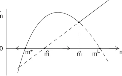
ferential equation (33) has a unique steady state atm∗, so that at the steady state monetary policy takes the form of a Taylor rule and inﬂation coincides with the target π∗. Figure 4 overimposes the phase diagrams corresponding to the interest rate feedback rule (ﬁgure 3)

Figure 4: The phase diagram of m under a monetary policy regime switch, Eqn. (33)

m

L

m*

m

~

m

^

m

⋅

0

and the money growth rate rule (ﬁgure 2). It is evident from ﬁgure 4 that in order for m∗

to be the unique steady state of (33), µ and ˜m must be such that m∗ <m < m < m˜ L_{. In}

turn, the restriction m∗ <m < m L _{requires setting} _µ _{as follows:}

πL < µ < π∗. (34)

To see why, note thatm∗,m, andmLare implicitly given by, respectively,um(y, m∗)/uc(y, m∗) =

r+π∗,um(y,m)/uc(y,m) =r+µ, and um(y, mL)/uc(y, mL) =r+πL.

However, not any value of ˜m in the interval (m, m L_{) guarantees the continuity of ˙}_m_{. This}

further requirement will be met only if at ˜m the right-hand sides of (27) and (29) are equal to each other. It is apparent from ﬁgure 4 and from our characterization of equations (27) and (29) that there exists at least one such value of real balances in the interval (m, m L). (Figure 4 is drawn under the assumption that there exists a unique such m). We pick any one of these values for real balances as the threshold for the monetary policy switch. The

(26)

solid line in ﬁgure 4 depicts the phase diagram of equation (33) when µ and ˜m are chosen so that m∗ is the only constant solution to that diﬀerential equation and ˙m is continuous.

The target level of real balances m∗ is not just a steady-state solution to (33) but indeed represents a perfect-foresight equilibrium. For, as we showed earlier, it satisﬁes the transver-sality condition (30). In addition tom∗, equation (33) admits a continuum of solutions that begin to the right of m∗ and converge to inﬁnity. However, none of these solutions can be supported as perfect-foresight equilibria because, as real balances cross the threshold ˜m, monetary policy switches from an interest-rate feedback rule to a money growth rate rule and real balances embark on an explosive path that, provided µ is nonnegative,10 violates the transversality condition (32).

We conclude that the proposed monetary regime switch is successful at ruling out the liq-uidity trap, preserving a Taylor rule around the target rate of inﬂation π∗, and guaranteeing the continuity of the price level and inﬂation.

6

Discussion and conclusion

The zero bound on nominal interest rates makes economies in which monetary policy takes the form of an interest-rate feedback rule prone to unintended equilibrium outcomes in which business cycles are driven by non-fundamental shocks. When these undesirable circumstances occur, the monetary authority finds itself powerless to bring about the policy objectives of the government. It is precisely this inability of monetary policy to affect key macroeconomic variables, such as the level of inflation and the volatility of output and prices that is at the heart of the concept of a liquidity trap.

Besides the explicit consideration of the zero bound on nominal interest rates, perhaps the most notable diﬀerence between our model and those that stress the desirability of Taylor rules is the absence of nominal rigidities. However, the possibility of falling into a liquidity

10_{The requirement} _µ _≥ _{0 calls, given (34), for} _π∗ _> _{0. It follows that the monetary policy switch is}

(27)

trap as a consequence of Taylor-type rules is not limited to the simple flexible-price environ-ment presented in this paper. In Benhabib, Schmitt-Grohé, and Uribe (2000), we show that Taylor rules also engender liquidity traps in environments with sluggish price adjustment. In this type of model, the liquidity trap involves indeterminacy not only of inflation and real balances, as in the model considered in this paper, but also of the level of aggregate demand. The policy recommendations aimed to eradicate liquidity traps proposed in sec-tions 4 and 5 are also effective in economies with sticky prices. For those recommendasec-tions involve the violation of a transversality condition in the event that the economy falls into a liquidity trap. The violation of this long-run restriction depends on the asymptotic behavior of the endogenous variables of the model, which is independent of short-run nominal price rigidities.

A further difference between the theoretical environment considered in this paper and that studied in part of the related literature is our treatment of time as a continuous variable. Again, neither the existence of a liquidity trap emerging as a consequence of the adoption of a Taylor rule nor the effectiveness of the proposed remedies is affected by this assumption in any important way. Schmitt-Grohé and Uribe (2000) analyze a discrete-time cash-in-advance model with cash and credit goods (which, as is well known, is equivalent to a money-in-the-utility-function model with money and consumption being Edgeworth complements), and show that a Taylor rule in combination with a lower bound on nominal rates gives rise to an unintended liquidity trap. Because the nature of this undesirable equilibrium is identical to that identified in this paper, the long-run restrictions that are capable of eliminating liquidity traps in the continuous-time model will also be applicable under discrete time.

Buiter and Panigirtzoglou (1999) have proposed the use of Gesell taxes on monetary balances as a way to avoid liquidity traps. A Gesell tax can be interpreted as a negative interest rate on money. Because the opportunity cost of holding money is given by the diﬀerence between the nominal rates of return on bonds and money, a Gesell tax allows the opportunity cost of holding money to be positive when nominal interest rates on government

(28)

bonds are negative. Thus, if a liquidity trap is understood as a situation in which the opportunity cost of holding money becomes zero, then a Gesell tax clearly does not eliminate it but simply pushes the nominal interest rate on bonds at which it occurs below zero.

Buiter and Panigirtzoglou argue, on empirical grounds, that the government’s ability to set negative interest rates on bonds reduces the likelihood that a liquidity trap will ever occur. They illustrate their idea by observing that if countries have a near-zero inﬂation target and if the long-run real interest rate settles at a level of around 2%, then a contractionary shock that calls for a reduction of the real interest rate of more than 2% would require the government to set the nominal interest rate below zero, which (in the absence of Gesell taxes) would be impossible.

The validity of this argument, however, hinges crucially on the assumption that the inflation target is not affected by the imposition of the Gesell tax. Such an assumption would be realistic if deviations of inflation from zero have large negative welfare effects, as is the case, for example, in some models of nominal price stickiness like the one presented in Calvo (1983), where both inflation and deflation exacerbate nominal price dispersion. However, another determinant of the inflation target maybe the government’s desire to set the inflation rate close to the one called for by the Friedman rule. This inflation rate falls one-for-one with the Gesell tax rate. Therefore, the extend to which a Gesell tax will reduce the likelihood of liquidity traps will be less the more weight the government assigns to the objective of implementing the Friedman rule.

More importantly, Gesell taxes fail to rule out the liquidity traps that arise as a conse-quence of Taylor-type monetary policy rules. What is important for the possibility of falling into a liquidity trap in this case is the combination of a Taylor-type interest-rate rule with the existence ofsome lower bound on nominal interest rates. Whether this bound is positive,

(29)

Appendix

Liquidity traps when the zero bound is binding

Consider a Taylor rule that stipulates a zero nominal interest rate for inflation rates below a certain threshold. Specifically, following Schmitt-Grohé and Uribe (2000), we will focus on a piecewise linear specification:

R(π) = max[0, r+π∗+γ(π−π∗)]; γ >1;π∗ >−r. (35) This interest-rate feedback rule speciﬁes an active monetary policy forπ > π ≡π∗−(r+π∗)/γ

and a passive one featuring a zero nominal interest rate for π < π. We wish to show that under this monetary policy rule in combination with the fiscal regime given by (12), liquidity traps continue to be a possible equilibrium outcome. For analytical convenience, we establish the existence of liquidity traps under two specific parameterizations of the instant utility function. The first specification is

u(c, m) =camb; a, b >0, a+b≤1, (36) which satisﬁes all the restrictions imposed on u in section 2.1. The second functional form is

u(c, m) = ln(m) + ln(c−m). (37)

This utility function displays a satiation point for real balances at m = c/2 and m ≡

min(m, c/2).

Assume ﬁrst that preferences are given by (36). Combining (4) and (5) yields a liquidity preference function of the form R= (b/a)(c/m). It is clear that there exists no steady state with ﬁnite m andR = 0. However, we will show that there exists a steady-state equilibrium

(30)

with π = π∗ and a continuum of non-steady-state equilibria in each of which the inflation rate starts in the interval (π, π∗) and converges to π. In the non-steady-state equilibria, the nominal interest rate converges to 0 without ever reaching that floor, and real balances converge to infinity at the rate r+ π. As long as π > π, we have, time-differentiating equation (4) and the liquidity preference function, that ˙λ/λ = bm/m˙ and ˙R/R = −m/m˙ , respectively. Then equation (15) takes the form

˙

π=− R(π)

bR(π)[r+π−R(π)]. Using the Taylor rule given in (35), this expression becomes

˙

π= r+π

∗₊_γ₍_π₋_π∗₎

bγ (γ−1)(π−π

∗₎_. ₍₃₈₎

The fact that the right-hand side of this expression is continuous and negative in the interval (π, π∗) and vanishes at π∗ and π implies that π∗ is a steady-state solution and that there exists a continuum of solutions starting in the interval (π, π∗) and converging toπ. Because, given the ﬁscal policy (12), the transversality condition (11) is always satisﬁed, all of these solutions represent perfect-foresight equilibria. Thus, liquidity traps cannot be ruled out.

One can show that the policies designed in sections 4 and 5 are also capable of eliminating liquidity traps under the interest-rate feedback rule (35) and the preference speciﬁcation given in (36).11 Of particular interest is the case of a balanced-budget rule studied in section 4.1. Recall that in order for this ﬁscal regime to be capable of eliminating the liquidity trap, it is necessary that limt→∞

t

0 R(s)ds <∞. Solving the diﬀerential equation (38) and

using the interest-rate feedback rule (35), the equilibrium path of the nominal interest rate associated with some π(0) ∈ (π, π∗) can be expressed as R(t) = (r+π∗) δ1e−δ2t

δ1e−δ2t−1, where δ₁ = 1 + _γ₍_πr₍₀₎+π₋∗_π_∗₎ < 0 and δ₂ = (r+π∗)(γ − 1)/(γb) > 0. Thus, limt→∞

t

0 R(s)ds =

11_{A switch to a money growth rate peg that eliminates the liquidity trap ensuring the continuity of}_P _and

πexists if one can ﬁndµ≥0 such that (µ−π∗)

r+µ 1+b −(γ−1)(r+π ∗₎ bγ <0.

(31)

(r+π∗) ln(1−δ₁)/δ₂ <∞.12

Consider now the utility function given in equation (37). In this case, there exist two steady-state equilibria, π =−r and π =π∗, and a continuum of non-steady-state equilibria in which the inflation rate originates in the interval (π, π∗) and converges to −r. To see that π = −r represents a perfect-foresight equilibrium, note that R(−r) = 0, so that in equilibrium m must be greater or equal to the satiation point y/2 and λ is constant and equal to 2/y. Since the transversality condition is always satisfied under the fiscal policy (12), all equilibrium conditions are satisfied.

If π > π, then equation (15) takes the form

˙

π=−2 +R(π)

γ [1 +R(π)][r+π−R(π)].

Clearly, π = π∗ represents a solution to this differential equation. In addition there exists an infinite number of solutions starting in the interval (π, π∗) that decline monotonically reaching π in finite time. At that point the above differential equation ceases to hold, m

reaches the satiation point y/2, R vanishes, and π jumps down to −r. Because under the ﬁscal regime (12), the transversality condition is always satisﬁed, all these trajectories as well as the steady state π=π∗ represent perfect-foresight equilibrium outcomes.

Again, one can show that the policies presented in sections 4 and 5 will rule out liquidity traps.13 In particular, under a balanced-budget requirement the liquidity trap can be ruled out because R(t) vanishes in ﬁnite time, so that limt→∞

t

0 R(s)ds <∞.

12_{Under different preference specifications whether this limit is finite or not will depend on the values}

taken by the parameters describing preferences and the interest rate feedback rule.

13_{The existence of a smooth switch to a money growth rate rule that eliminates the liquidity trap requires}

(32)

References

Benhabib, Jess, Stephanie Schmitt-Groh´e, and Mart´ın Uribe “Monetary Policy and Multiple Equilibria,” 1999, The University of Pennsylvania.

Benhabib, Jess, Stephanie Schmitt-Groh´e, and Mart´ın Uribe, “The Perils of Taylor Rules,”

Journal of Economic Theory, , (2000): forthcoming.

Bernanke, Ben and Michael Woodford, “Inﬂation Forecasts and Monetary Policy,” Journal

of Money Credit and Banking, 29, (1997): 653-684.

Brock, William A., “Money and Growth: The Case of Long Run Perfect Foresight,”

Inter-national Economic Review, 15, (October 1974): 750-777.

Brock, William A., “A Simple Perfect Foresight Monetary Model,” Journal of Monetary

Economics, 1, (April 1975): 133-150.

Buiter, Willem and Nikolaos Panigirtzoglou “Liquidity Traps: How to Avoid Them and How to Escape Them,” August 1999, CEPR Discussion Paper No. 2203.

Calvo, Guillermo A., “Staggered Prices in a Utility-Maximizing Framework,” Journal of

Monetary Economics, 12, (1983): 383-398.

Clarida, Richard, Jordi Gal´ı, and Mark Gertler “Monetary Policy Rules and Macroeconomic Stability: Evidence and Some Theory,” 1997, NBER working paper No. 6442.

Clarida, Richard, Jordi Gal´ı, and Mark Gertler, “Monetary policy rules in practice: some international evidence,” European Economic Review, 42, (1998): 1033-1067.

Fuhrer, Jeﬀrey C. and Brian F. Madigan, “Monetary Policy When Interest Rates Are Bounded At Zero,” Review of Economics and Statistics, , (November, 1997): 573-585.

Krugman, Paul R., “It’s Baaack: Japan’s Slump and the Return of the Liquidity Trap,”

Brookings Papers on Economic Activity, 0, (1998): 137-87.

Leeper, Eric, “Equilibria under ‘Active’ and ‘Passive’ Monetary and Fiscal Policies,” Journal

of Monetary Economics, 27, (1991): 129-147.

Levin, Andrew, Volker Wieland, and John Williams “Robustness of Simple Policy Rules Un-der Model Uncertainty” In Monetary Policy Rules, edited by John B. Taylor, University

(33)

of Chicago Press, 1999.

Obstfeld, Maurice and Kenneth Rogoﬀ, “Speculative Hyperinﬂations in Maximizing Models: Can We Rule Them Out?,” Journal of Political Economy, 91, (August 1983): 675-687.

Orphanides, Athanasios and Volker Wieland “Price Stability and Monetary Policy Eﬀec-tiveness When Nominal Interest Rates Are Bounded At Zero,” Finance and Economic Discussion Series, 98-35, Board of Governors of the Federal Reserve System, June 1998. Rotemberg, Julio and Woodford, Michael “Interest-Rate Rules in an Estimated Sticky-Price

Model” InMonetary Policy Rules, edited by John B. Taylor, University of Chicago Press,

1999.

Reifschneider David and John Williams “Three Lessons for Monetary Policy in a Low In-ﬂation Era,” Finance and Economic Discussion Series, 99-44, Board of Governors of the Federal Reserve System, August 1999.

Schmitt-Groh´e, Stephanie and Mart´ın Uribe, “Price Level Determinacy and Monetary Policy Under a Balanced-Budget Requirement,” Journal of Monetary Economics, 45, (February

2000): forthcoming.

Shigoka, Tadashi, “A Note on Woodford’s Conjecture: Constructing Stationary Sunspot Equilibria in a Continuous Time Model,” Journal of Economic Theory, 64, (December,

1994): 531-540.

Taylor, John B., “Discretion versus rules in practice,” Carnegie-Rochester Series on Public

Policy, 39, (1993): 195-214.

Wolman, Alexander L. “Real Implications of the Zero Bound on Nominal Interest Rates,” mimeo Federal Reserve Bank of Richmond, December 1999.

Woodford, Michael, “Monetary policy and price level determinacy in a cash-in-advance econ-omy,” Economic Theory, 4, (1994): 345-380.