Analytical models for high performance milling. Part I: Cutting forces, structural deformations and tolerance integrity

(1)

International Journal of Machine Tools & Manufacture 46 (2006) 1478–1488

Analytical models for high performance milling. Part I: Cutting forces,

structural deformations and tolerance integrity

E. Budak

Faculty of Engineering and Natural Sciences, Sabanci University, Istanbul, Turkey

Received 15 July 2005; received in revised form 17 September 2005; accepted 22 September 2005 Available online 8 November 2005

Abstract

Milling is one of the most common manufacturing processes in industry. Despite recent advances in machining technology, productivity in milling is usually reduced due to the process limitations such as high cutting forces and stability. If milling conditions are not selected properly, the process may result in violations of machine limitations and part quality, or reduced productivity. The usual practice in machining operations is to use experience-based selection of cutting parameters which may not yield optimum conditions. In this two-part paper, milling force, part and tool deﬂection, form error and stability models are presented. These methods can be used to check the process constraints as well as optimal selection of the cutting conditions for high performance milling. The use of the models in optimizing the process variables such as feed, depth of cut and spindle speed are demonstrated by simulations and experiments.

Keywords:Milling forces; Form errors; End mill; Deﬂections

1. Introduction

Milling is a very commonly used manufacturing process in industry due to its versatility to generate complex shapes in variety of materials at high quality. Due to the advances in machine tool, CNC, CAD/CAM, cutting tool and high speed machining technologies in last couple of decades, the volume and importance of milling have increased in key industries such as aerospace, die and mold, automotive and component manufacturing. Despite these developments, the process performance is still limited, and the full capability of the available hardware and software cannot be realized due to the limitations set by the process. The purpose of this two-part paper is to give an overview of the analytical methods that can be used to maximize the productivity in milling without violating the machine limitations and part quality requirements. The ﬁrst part will focus on the milling force, deﬂection and form error modeling whereas the models of chatter stability and avoidance with high material removal rate will be presented in the second part.

Cutting force is the most fundamental, and in many cases the most significant parameter in machining opera-tions. In milling processes, they also cause part and tool deflections which may result in tolerance violations. Due to the complexity of the process geometry and mecha-nics compared to turning, milling process models appeared later than some of the pioneering work done on the orthogonal cutting [1]. In one of the very early studies, Martelotti [2] analyzed and modeled the complex geo-metry and relative part-tool motion in milling. Later, Koenigsberger and Sabberwal [3] developed equations for milling forces using mechanistic modeling. The mechanistic approach has been widely used for the force predictions and also been extended to predict associated machine component deflections and form errors [4–8]. Another alternative is to use mechanics of cutting approach in determining milling force coefficients as used by Armarego and Whitfield[9]. In this approach, an oblique cutting force model together with an orthogonal cutting database is used to predict milling force coeffi-cients [10]. This approach was applied to the cases of complex milling cutter geometries and multi-axis milling operations[11–13].

www.elsevier.com/locate/ijmactool

_{Tel.: +902164839519; fax: +902164839550.} E-mail address:[email protected].

(2)

In this paper, milling force, structural deformation, form error prediction and control models are presented. Experi-mental results are also given to demonstrate the applica-tions of these models. The models can be used to check the constraints such as available machine power or allowable form errors, and determine the high performance milling conditions.

2. Milling process geometry and force modeling

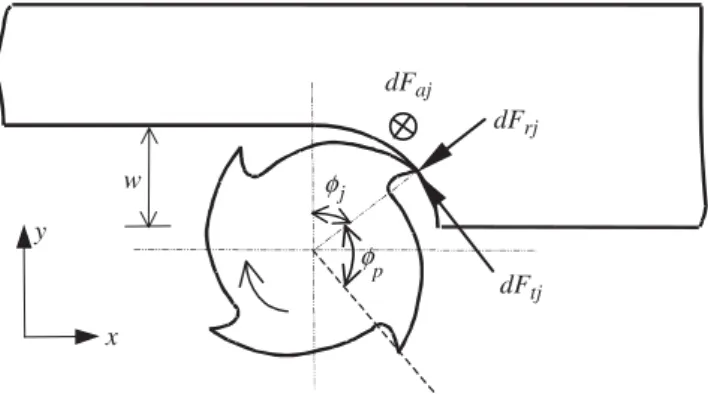
Milling forces can be modeled for given cutter geometry, cutting conditions, and work material. Two different methods will be presented for the force analysis: Mechan-istic and mechanics of cutting models which differ in the way the cutting force coefﬁcients, which relate the cut chip area to the fundamental milling force components, shown inFig. 1are determined.

2.1. Mechanistic force model

In mechanistic force model, cutting force coefﬁcients are calibrated for certain cutting conditions using experimental data. However, the same milling force model can be used for both mechanistic and mechanics of cutting models. Consider the cross-sectional view of a milling process shown in Fig. 1. For a point on the (jth) cutting tooth, differential milling forces corresponding to an inﬁnitesimal element thickness (dz) in the tangential, dFt, radial, dFr, and axial, dFa, directions can be given as

dFtjðf;zÞ ¼Kthjðf;zÞdz,

dFrjðf;zÞ ¼KrdFtjðf;zÞ,

dFajðf;zÞ ¼KadFtjðf;zÞ, ð1Þ

wherefis the immersion angle measured from the positive

y-axis as shown inFig. 1. The axial force component,Fa, is in the axial direction of the cutting tool, which is perpendicular to the cross-section shown in Fig. 1. In Eq. (1), the edge forces are also included in the cutting force coefﬁcient which is usually referred to as the exponential force model. They are separated from the cutting force coefﬁcients in edge force or linear-edge force

model [10,14]:

dFtjðf;zÞ ¼ ½KteþKtchjðf;zÞdz,

dFrjðf;zÞ ¼ ½KreþKrchjðf;zÞdz,

dFajðf;zÞ ¼ ½KaeþKachjðf;zÞdz, ð2Þ

where subscripts (e) and (c) represent edge force and cutting force coefﬁcients, respectively. The radial (w) and axial depth of cut (a), number of teeth (N), cutter radius (R) and helix angle (b) determine what portion of a tooth is in contact with the work piece for a given angular orientation of the cutter,f¼Ot, wheretis the time,Ois the angular speed in (rad/s) or O¼2pn=60, n being the (rpm) of the spindle. The chip thickness at a certain location on the cutting edge can be approximated as follows:

hjðf;zÞ ¼ft sinfjðzÞ, (3)

where ftis the feed per tooth and fj(z) is the immersion

angle for the ﬂute (j) at axial positionz. Due to the helical ﬂute, the immersion angle changes along the axial direction as follows:

fjðzÞ ¼fþ ðj1Þfp

tanb

R z, (4)

where the pitch angle is deﬁned as f_p¼2p=N. The tangential, radial and axial forces given by Eqs. (1) and (2) can be resolved in the feed,x, normal,y, and the axial direction, z, and can be integrated within the immersed part of the tool to obtain the total milling forces applied on each tooth. For the exponential force model, the following is obtained after the integration:

FxjðfÞ ¼

KtftR

4 tanb½cos 2fjþKrð2fjðzÞ sin 2fjðzÞÞ zjuðfÞ zjlðfÞ, FyjðfÞ ¼ KtftR 4 tanb½ð2fjðzÞ sin 2fjðzÞÞ þKrcos 2fjðzÞ zjuðfÞ zjlðfÞ, FzjðfÞ ¼ KaKtftR tanb ½cosfjðzÞ zjuðfÞ zjlðfÞ, ð5Þ

where zjl(f) and zju(f) are the lower and upper axial engagement limits of the in cut portion of the ﬂute j. The engagement limits depend on the cutting and the tool geometries f_stðzÞ ¼pcos1 1w R ðdown millingÞ, f_exðzÞ ¼cos1 1w R ðup millingÞ. ð6Þ

Note that fex is always p in down milling and fst is always 0 in up milling according to the convention used in Fig. 1. The helical cutting edges of the tool can intersect this area in different ways resulting in different integration limits which are given in [14,15]. The total milling forces

φj y x w dFrj dFtj dFaj φ_p

(3)

can then be determined as FxðfÞ ¼ XN j¼1 FxjðfÞ; FyðfÞ ¼ XN j¼1 FyjðfÞ, FzðfÞ ¼ XN j¼1 FzjðfÞ. ð7Þ

The cutting torque and power due to the tooth j can easily be determined from Eqs. (1) and (3) as follows:

TjðfÞ ¼ KtftR2 tanb ½cosf zjuðfÞ zjlðfÞ, PjðfÞ ¼OTjðfÞ. ð8Þ

The total torque and power due to all cutting teeth can be determined similar to the summation for the forces given Eq. (7). Maximum value of the forces, torque and power can be determined after one full revolution of the tool, i.e.,f: 0–2p, is simulated.

For the linear-edge force model, the forces are obtained similarly by using Eq. (2), and integrating within the engagement limits as follows[10]:

FxjðfÞ ¼

R

tanb Kte sinfjðzÞ KrecosfjðzÞ þ

f_t 4 ½Krcð2fjðzÞ sin 2fjðzÞÞ Ktc cos 2fjðzÞ zju zjl , FxjðfÞ ¼ R

tanb KresinfjðzÞ Kte cosfjðzÞ þ

f_t 4 ½Ktcð2fjðzÞ sin 2fjðzÞÞ Krccos 2fjðzÞ zju zjl , FxjðfÞ ¼ R tanb½KaefjðzÞ ftKaccosfjðzÞ zju zjl, ð9Þ

The forces given by Eqs. (5) and (8) can be used to predict the cutting forces for a given milling process if the milling force coefﬁcients are known. As mentioned in the beginning of this section, in the mechanistic models the force coefﬁcients are calibrated experimentally which is explained in the following section.

2.2. Identification of milling force coefficients

In mechanistic force model, milling force coefﬁcientsKt,

Kr and Ka can be determined from the average force expressions [10]as follows: Kr¼ P ¯FyQ ¯Fx P ¯FxþQ ¯Fy , Kt¼ ¯ Fx f_tðPQKrÞ , Ka¼ ¯ Fz f_tKtT , ð10Þ where P¼ aN 2p½cos 2f fex fst, Q¼ aN 2p½2fsin 2f fex fst, T¼ aN 2p½cosf fex fst. ð11Þ

The average forces, F¯x; F¯y and F¯z, can be obtained

experimentally from milling tests. In exponential force model, the chip thickness affects the force coefﬁcients. Since the chip thickness varies continuously in milling, the average chip thickness,ha, is used:

ha¼ft

cosf_stcosf_st

f_exf_st . (12)

In calibration tests, the usual practice is to conduct experiments at different radial depths and feed rates in order to cover a wide range ofhafor a certain tool–material pair. The force coefﬁcients can then be expressed as following exponential functions:

Kt ¼KThpa ,

Kr¼KRhqa ,

Ka¼KAhsa , ð13Þ

whereKT, KR, KA, p, qandsare determined from the linear regressions performed on the logarithmic variations ofKt,

Kr,Kawithha.

In linear-edge force model the total cutting forces are separated into two parts: edge forces and cutting forces. The edge force represents the parasitic part of the forces which are not due to cutting, and thus do not depend on the uncut chip thickness whereas cutting forces do. Then, the average forces can be described as follows:

¯

Fq¼F¯qeþftF¯qc ðq¼x;y;zÞ, (14)

where the edge and cutting components of the average forcesðF¯qe; F¯qcÞare determined using the linear regression

on the average measured milling forces. The milling force coefﬁcients for the linear-edge force model can be obtained from the average forces similar to the exponential force model as follows: Ktc¼4 ¯ FxcPþF¯ycQ P2_þ_Q2 ; Krc¼ KtcP4F¯xc Q ; Kac¼ ¯ Fzc T , Kte¼ ¯ FxeSþF¯yeT S2þT2 ; Kre¼ KteSþF¯xe T , Kae¼ 2p aN ¯ Fze f_exf_st, ð15Þ

whereP,QandTare given by Eq. (11), and

S¼aN 2p½sinf

fex fst.

(4)

2.3. Mechanics of milling force model

The mechanistic force models introduced in the previous section yield high accuracy force predictions for most applications. However, since the cutting force coefficients must be calibrated for each tool–material pair covering the conditions that are of interest, this approach may some-times be very time consuming. In this sense, mechanics of milling approach is more general and may reduce the number of tests significantly. The basic idea in this approach is to use analytical cutting models relating the chip area to the cutting forces, and to determine the parameters required in the model experimentally when necessary. In case of milling an oblique cutting model has to be employed due to helical flutes.

In oblique cutting models, there are several important planes which are used to measure tool angles and write down velocity and force equilibrium relations [16]. The normal plane, which is perpendicular to the cutting edge, is commonly used in the analysis. After several assumptions, and velocity and the force equilibrium equations, the following expressions are obtained for the cutting force coefﬁcients in an oblique cutting process:

Ktc¼ t

sinf_n

cosðg_nanÞ þtanZ_csing_n tanb

c , Krc¼ t sinf_ncosb sinðgnanÞ c , Kac¼ t sinfn

cosðg_nanÞtanbtanZc singn

c , ð16Þ wherec¼ ffiffiffiffiffiffiffiffiffiffiffiffiffiffiffiffiffiffiffiffiffiffiffiffiffiffiffiffiffiffiffiffiffiffiffiffiffiffiffiffiffiffiffiffiffiffiffiffiffiffiffiffiffiffiffiffiffiffiffiffiffiffiffiffiffiffiffiffiffiffi cos2_ð_f nþgnanÞ þtan2Zcsin2gn q .

In Eq. (16), (t) is the shear stress in the shear plane,fnis the shear angle in the normal plane, b is the angle of obliquity or helix angle and Zc is the chip ﬂow angle measured on the rake face. The chip ﬂow angle can be solved iteratively based on the equations obtained from force and velocity relations [9,10,14]. However, for simplicity, Stable’s rule[17]may also be used which states that ZcEb. gn and an are the friction angle and the rake angle in the normal plane, respectively, and are given by [16]

tangn¼tangcosZc; tanan¼tanarcosb, (17)

wherearis the rake angle measured in the velocity plane, which is normal to the tool axis, andgis the friction angle on the rake face.

The procedure proposed by Armarego and Whitfield[9], and later by Budak et al.[10]for the prediction of milling force coefficients will be briefly described here. First of all, the required data is obtained from the orthogonal cutting tests in order to reduce the number of variables, thus the number of tests, and to generate a more general database which can be used for other processes as well. The shear angle, shear stress and friction coefficient can be obtained

from orthogonal cutting tests as follows [9,10]: tanf¼ rcosa

1rsina,

t¼ ðFpcosfFqsinfÞsinf

bt ,

tang¼ FqþFp tana

FpFq tana

, ð18Þ

where ris the cutting ratio or the ratio of the uncut chip thickness to the chip thickness, ais the rake angle,Fpand

Fq are the cutting forces in the cutting speed and the feed direction, respectively. If the linear-edge force model is to be used then the edge cutting force components must be subtracted from the cutting forces measured in each direction using linear regression [14]. The edge force coefficients are identified from the edge cutting forces. After the orthogonal cutting tests are repeated for a range of cutting speed, rake angle and uncut chip thickness, an orthogonal cutting database is generated for a certain tool and work material pair. These data can then be used to determine the milling cutting force coefficients using the oblique model given by Eq. (16). The force coefficients and the milling forces predicted using this approach have been demonstrated to be very close to the milling experiment results[10,14].

2.4. Example application

As a demonstration of the force models presented here, a titanium (Ti6Al4V) milling example is considered. First of all, an orthogonal cutting database is generated using carbide tools with different rake angles, at different speeds and feedrates[10,14]:

t¼613 MPa; b¼19:1þ0:29a,

r¼r0ha; r0¼1:7550:028a; a¼0:3310:0082a,

Kte¼24 N=mm; Kre¼43 N=mm:

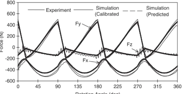
In addition, many test were conducted to calibrate the milling force coefficients directly from the milling tests. Budak et al. [10] and Budak[14] showed that there is, in general, a good agreement between the predicted and the identified cutting force coefficients using this approach. As an example, the predictions for one of the cases are shown inFig. 2together with the measured milling forces for one full rotation of the cutter. This is a half-immersion up milling test performed using a 301helix, 19.05 mm diameter and four-fluted end mill with 121 rake angle. The axial depth of cut is 5 mm, and 0.05 mm/tooth feed was used at 30 m/min cutting speed. The measured and the predicted cutting forces using the force coefficients identified from the milling tests and calculated using the oblique model in all three directions are shown in the figure. As it can be seen from this figure, the predictions are very close to the measured forces. The models were tested for many cases and good results were obtained[10].

(5)

3. Deﬂections and form errors

3.1. Surface generation

In peripheral milling the work piece surface is generated as the cutting teeth intersect the finish surface. These points are called thesurface generation pointsas shown inFig. 3. As the cutter rotates, these points move along the axial direction due to the helical flutes, completing the surface profile at a certain feed position along thex-axis.

The surface generation points zcj corresponding to a

certain angular orientation of the cutter, f, can be determined from the following relation:

f_jðzcjÞ ¼fþjfp

tanb

R ¼

0 for up milling; p for down milling:

(

(19) The surface generation points can then be resolved from above equation as follows:

zcjðfÞ ¼

Rðfþjf_pÞ

tanb for up milling;

zcjðfÞ ¼

Rðfþjf_ppÞ

tanb for down milling: ð20Þ

As the surface is generated point by point by different teeth resulting inhelix markson the surface, in helical end milling the surface finish is not as good as the finish that would be obtained by a zero-helix tool. In case of non-helical end milling, the whole surface profile at a certain feed location is generated by a single tooth as the immersion angle does not vary along the axial direction. Thus, the helix marks do not exits with zero-helix end mills, and a better surface finish is obtained. However, helical flutes result in much smaller force fluctuations, lower peak forces, and thus smoother cutting action with reduced impacts. In addition, helical flutes improve chip evacua-tion.

The deﬂections of the tool and the work piece in the normal direction to the ﬁnish surface are imprinted on the

surface resulting in form errors which are analyzed the next.

3.2. Form errors in peripheral milling

The form error can be defined as the deviation of a surface from its intended, or nominal, position. In case of peripheral milling, the deflections of the tool and the part in the direction normal to the finished surface cause the form errors as shown inFig. 3. Then, the total form error at a certain position on the surface,e(x,z), can be written as follows:

eðx;zÞ ¼dyðzÞ ypðx;zÞ, (21)

wheredy(z)is the tool deﬂection at an axial positionz, and

yp(x,z)is the work deﬂection at the position (x,z).

3.2.1. Structural model of the tool

Several modeling approached can be used to determine the end mill deﬂections which will be summarized here.

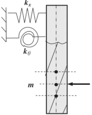
3.2.1.1. Cantilever beam model. The end mill can be modeled as a beam with clamping stiffness as shown in Fig. 4. kx and ky represent the linear and torsional clamping stiffness at the holder–tool interface. They can be identiﬁed experimentally for a certain tool–holder pair [8,18].

The cutting tool is divided intonelements along the axial direction. The normal force in themth element,fym, can be

written as f_ymðfÞ ¼ KtftR 4 tanb XN j¼1 ð2f_jðzÞ sin 2f_jðzÞÞ h þKr cos 2fjðzÞ izm zm1 , ð22Þ

where zm represents the axis boundary of the cutter in

elementmshown inFig. 4. The elemental cutting forces are equally split by the nodesmand (m1) bounding the tool element (m1). The deﬂection at a node k caused by the

yp(x,z)

δ

y(z) surface generation points x y z

Fig. 3. Surface generation in peripheral milling. -600 -400 -200 0 200 400 600 800 0 45 90 135 180 225 270 315 360 Rotation Angle (deg)

Force (N) Fx Fy Experiment Simulation (Calibrated Simulation (Predicted Fz

Fig. 2. Predicted and the measured milling forces for the example in Section 2.4.

(6)

force applied at the nodemis given by the cantilever beam formulation as[8,14]: dyðk;mÞ ¼ f_ymz2 m 6EI ð3umukÞ þfym kx þfymumuk ky for 0oukoum, dyðk;mÞ ¼ f_ymu2 m 6EI ð3ukumÞ þ f_ym kx þfymumuk ky for umouk, ð23Þ

whereEis the Young’s modulus, Iis the area moment of inertia of the tool,uk¼Lzk,Lbeing the gauge length of

the cutter. The total static defection at the nodal stationk

can be calculated by the superposition of the deﬂections produced by all (n+1) nodal forces:

dyðkÞ ¼

Xnþ1 m¼1

dyðk;mÞ. (24)

The tool deﬂections at the surface generation points can be determined from Eq. (6) and substituted into Eq. (3) to determine the form errors.

3.2.1.2. Segmented beam model. The area moment of inertia must take the affect of the flutes into account. Use of an equivalent tool radius, Re¼sR, where s¼0.8 for common end mill geometries was demonstrated to yield reasonably accurate predictions by Kops and Vo[19]. An improved method of tool compliance modeling is given by Kivanc and Budak [18] where end mill deflections were approximated using a segmented beam model. For such a case, if a load is applied at the tip of the tool the maximum deflection is given by[20] ymax¼ FL13 3EI1þ 1 6 FL1ðL2L1ÞðL2þ2L1Þ EI2 þ1 6 FL2ðL2L1Þð2L2þL1Þ EI2 , ð25Þ

whereD1 is the mill diameter,D2 is the shank diameter,L1 is the ﬂute length, L2 is the overall length, Fis the point

load,I1andI2 are the moment of inertias of the fluted and unfluted parts, respectively. In case of distributed forces and existence of clamping stiffness, a formulation similar to Eq. (23) can be derived. Due the complexity of the cutter cross-section along its axis, the inertia calculation is the most difficult aspect of the static analysis. The cross-sections of some end mills are as shown in Fig. 5.

In order to determine the inertia of the whole cross-section, inertia of region 1 is ﬁrst derived, and inertia of the other regions are obtained by transformation [21]. The total inertia of the cross-section is then obtained by summing the inertia of all regions. The inertia of region 1 is derived by computing equivalent radiusReqin terms of the radiusrof the arc and position of the center of the arc (a)[21]:

Req4-fluteðyÞ ¼asinðyÞ þ

ffiffiffiffiffiffiffiffiffiffiffiffiffiffiffiffiffiffiffiffiffiffiffiffiffiffiffiffiffiffiffiffiffiffiffiffiffiffiffiffiffiffi

ðr2_a2_{Þ þ}_a2_sin2 ðyÞ

q

; 0oypp=2,

Req3-fluteðyÞ ¼acos yþ p 3 þ ffiffiffiffiffiffiffiffiffiffiffiffiffiffiffiffiffiffiffiffiffiffiffiffiffiffiffiffiffiffiffiffiffiffiffiffiffiffiffiffiffiffiffiffiffiffiffiffiffiffiffi ðr2_a2_{Þ þ}_a2_cos2_ð_y_þp 3Þ r ; 0oyp2p=3,

Req2-fluteðyÞ ¼ acosðyÞ þ

ffiffiffiffiffiffiffiffiffiffiffiffiffiffiffiffiffiffiffiffiffiffiffiffiffiffiffiffiffiffiffiffiffiffiffiffiffiffiffiffiffiffiffi

ðr2_a2_{Þ þ}_a2_cos2_ð_y_Þ

p

; 0oypp: ð26Þ The moment of inertia of region 1 of a four-ﬂute end mill aboutx- and y-axis can be written as

Ixx4-flute¼ Z p=2 0 Z Req4-fluteðyÞ 0 r3sin2ðyÞdrdy " # 1 8p fd 2 4 þpðfd=2Þ 2 2 rþa fd 2 2 " # , Iyy4-flute¼ Z p=2 0 Z Req4-fluteðyÞ 0 r3cos2ðyÞdrdy " # 1 8p fd 2 4 " # , ð27Þ where 0orpReq(y). The same formulation can be written for region 1 of the 3- and 2-ﬂute tool. After transforming the inertia of region 1, the total inertias are found as follows:

Ixx4-flute;TOT¼Iyy4-flute;TOT¼2ðIxx4-fluteþIyy4-fluteÞ,

Ixx3-flute;TOT¼Iyy3-flute;TOT¼1:5ðIxx4-fluteþIyy4-fluteÞ,

Ixx2-flute;TOT¼2ðIyy2-fluteÞ; Iyy2-flute;TOT¼2ðIyy2-fluteÞ, ð28Þ

3.2.1.3. Finite elements modeling. In order to verify and improve the accuracy of analytical model predictions, ﬁnite elements analysis, FEA, is also used for tool deﬂections.

2 2 2 3 3 4 1 1 1 fd fd _fd

Fig. 5. Cross-sections of 4-, 3- and 2-ﬂute end mills.

kx

k

m

(7)

Approximately sixty tools with different configurations were simulated. Although FEA can be very accurate, it can also be very time consuming for each tool configuration in a virtual machining environment. Therefore, simplified equations were also derived to predict deflections of tools for given geometric parameters and density:

deflectionmax¼C F E L13 D14þ ðL23L13Þ D24 N , (29)

where F is the applied force and E is the modulus of elasticity (MPa) of the tool material. The geometric properties of the end mill are in millimeters. The constant

Cis 9.05, 8.30 and 7.93 andNis 0.950, 0.965 and 0.974 for 4-, 3- and 2-Flute cutters, respectively.

3.2.2. Clamping stiffness

After the tool is modeled accurately, the clamping stiffness must also be known for the total tool deflection. Depending on the tool and clamping conditions, the contribution of the clamping flexibility to the total deflection of the tool can be significant. There is not a model available in the literature for modeling of the tool clamping stiffness. However, a model given by Rivin [22] for the stiffness of cylindrical connections can be utilized. According to this model, the initial interference-fit pres-sures in the connection create a pre-loaded system, which is generally shaped by the applied clamping torque. Since the contact area is a function of tool diameter and contact length, the magnitudes of the interference displacements can be related to them. The elastic displacement in the connection can be determined as[22]

d¼2cq

pd , (30)

where c is the contact compliance coefﬁcient, q¼F=L is the force per contact length and d is the tool diameter. Therefore, the clamping stiffness can be expressed as

k¼F

m₌_n

d ¼

pLd

2c , (31)

wherenis a constant used to compensate the effect of the small lengths of contact. If Lo30, then this constant should be equal to 3, otherwise n¼2. The effect of using different materials for tools is represented by m. For carbide it is taken as 1 and for HSS tools it is 0.9. Coefﬁcient c should be experimentally determined for a connection. In other words,cis the ratio of the deﬂection representation to the force representation and it is constant for a type of tool holder:

c¼drep Frep , (32) where drep¼dpd, Frep¼ 2Fm nL . ð33Þ

After many static deﬂection tests with different clamping conditions,cwas determined to be approximately 0.07 for holders without collets such as power chucks and shrink ﬁt holders whereas for collet type holderscchanges substan-tially (0.05–0.15) depending on the type of the collet.

3.2.3. Structural model of the work piece

Work pieces deflect under cutting forces contributing to form errors. In general, the finite-element method (FEM) can be used to determine the structural deformations of the work piece. The elemental cutting forces in the normaly -direction given by Eq. (22) are to be used as the force vector. For the cases where the part is very thin such as a turbine blade or a thin plate, the change in the structural properties of the work piece due to removed material can be very important for accurate prediction of the deflections [8,14]. In addition, the tool–work contact and thus the force application points change as the tool moves along the feed direction. Therefore, the form error due to work piece deflections in milling require that the FE solutions be repeated many times in order to consider these special effects, i.e. varying part thickness and force location.

Fig. 6 shows the work piece model which is used by Budak and Altintas [8] and Budak [14] for deﬂection calculations. The part thickness is reduced fromtutotcat the cutting zone where the cutter enters the part at pointB

and exits at point A in down milling mode. The nodal forces on the tool are applied in the opposite direction on the corresponding nodes in the cutting zone. For a down milling case, the cutting teeth on an end mill with a positive helix angle enters the cut at the bottom of the part where it is the most rigid. As the tool rotates, the contact points move along the axial direction where tool deflections are much smaller. For a plate-like structure, however, these are the most flexible sections of the part resulting in high work piece deflections. Therefore, depending on the application, both part and tool deflections can be very significant and must be included in the calculations. The form error

b B n A K 1 2 cutter exit cutter entry B A 1 t c t u

(8)

calculations at a certain location of the tool result in the surface proﬁle at that position. After repeating this at many locations along the feed direction, the complete form error map of the surface is obtained.

3.3. Structure–process interaction

Part and tool deflections affect the cutting process in two ways. The deflections in the chip thickness direction will change the actual value of the chip thickness. However, due to the continuous feed motion, the chip thickness will approach to its intended value in a few tooth periods[23]. For most of the finishing operations, the radial depth of cut is very small in order to reduce forces, deflections, and thus the form errors. The deflections will change the radial depth of cut, and thus the start and exit immersions angles,

fstandfex, as follows: fstðzÞ ¼pcos1 1 wfðzÞ R down milling; f_exðzÞ ¼cos1 1wfðzÞ R up milling: ð34Þ

The effective start and exit angles vary along the axial,z -direction as the actual value of the desired width of cut,w, changes due to deﬂections:

wfðzÞ ¼wþdyðzÞ ypðx;zÞ. (35)

The effectives start and exit angles given by Eq. (34) must be used in the force and form error predictions for accurate results when the deﬂections are comparable to the radial depth of cut. The force model which includes these effects was named as flexible force model by Budak and Altintas[8]and Budak[14]. The solution is an iterative one as the deﬂections and forces depend on each other.

3.4. Example application

Peripheral milling of a cantilever plate made out of titanium (Ti6Al4) is considered [8,14]. The plate is very

flexible with dimensions of 64342.45 mm. Its flexibility is further increased by reducing the thickness by 0.65 mm down to 1.8 mm in a single milling pass, i.e. the axial depth of cut is 34 mm. A 19 mm carbide end mill with 301helix and single flute was used in order to eliminate run out effects. The tool gauge length is 55.6 mm and the linear clamping stiffness was measured to be 19.8 kN/mm where the torsional clamping stiffness was negligible. In order to constrain deflections and eliminate work–tool separation, a very small feed rate of ft¼0.008 mm/tooth was used. The cutting force coefficients were identified from the milling tests using the exponential force model:

KT¼207ðMPaÞ; p¼0:67; KR¼1:39; q¼0:043.

The Young’s Modulus of the tool and work materials are 620 and 110 GPa, respectively. Experimentally measured and simulated form errors on the plate are shown inFig. 7. Only the flexible force model predictions are shown as the deflections are very high compared to the radial depth. The form error at the cantilevered edge of the plate is due to the tool deflection, and it is approximately 30mm. The maximum form error occurs close to the free end of the plate where it is most flexible. The error increases from the start of the milling at the left side to the end due to the reduced thickness and increased flexibility of the plate. The rigid model, where the deflection–process interaction is neglected, overestimates the form errors significantly, about 150mm at the maximum error location [8]. The flexible model predictions agree with the measurements as shown in the figure.

4. Control and minimization of form errors

4.1. Feedrate scheduling

In machining operations, the usual practice is to use a constant feed rate for a machining cycle. In cases where there are tolerance violations due to excessive deﬂections, the feed may have to be reduced in the whole cycle even the maximum form error occurs only at a speciﬁc location.

500 400 300 200 100

Surface Error (mic)

0 500 400 300 200 100

Surface Error (mic)

0 31 21 11 Axial Depth -z (mm) 1 10 20 30 Axial Depth -z (mm) 0 60 50 40 30 20 10 0 10 20 30 40 50 60 0 Food Direction (mm) Food Direction (mm)

(9)

Feed rate scheduling method proposed by Budak and Altintas[8]can be used to constraint form errors reducing cycle times. This method is based on estimation of the maximum allowable feed rate for a speciﬁed dimensional tolerance. As in general the form errors vary along the tool path, different feed rates are obtained for different locations. The algorithm is an iterative one since the relation between the forces, and thus the deﬂections, and the chip thickness is not linear in exponential force model. For a dimensional tolerance value of (T) and feed location

x, the feed rate at an iteration stepmcan be determined as follows:

f₁ðx;mÞ ¼f₁ðx;m1Þ T

emaxðxÞ

, (36)

whereemax(x)is the maximum dimensional error obtained in iteration step m1. The starting value of the feed rate can be taken as the feed rate determined in the previousx

location. After all feeds are determined along the tool path, the total machining time can be calculated. In a simulation program, different radial depths can be used to identify the milling conditions for minimum machining time[8].

4.2. Milling conditions for minimized form errors

In precision milling of highly flexible systems deflections can be very high, and in order to maintain tolerance integrity of the part, slow feed rates, and thus small material removal rates (MRR) may have to be used resulting in low productivity. However, it may be possible to determine milling conditions which minimize form errors without sacrificing the productivity. It was demon-strated by Budak and Altintas[7]that the conditions which result in almost zero form error and with very high MRR can be determined. Material removal rate per revolution, MPR,can be used as a measure of the productivity:

MPR¼awf_tN, (37)

whereftis the feed rate per tooth,Nis the number of teeth on the cutter,aandware the axial and radial depth of cuts, respectively. The above equation indicates that the material removal rate is linearly proportional to the feed rate and depth of cuts. The relations between the force and the surface errors, and the cutting conditions, on the other hand, are nonlinear. Therefore, it may be possible to determine wand ftwhich produce the required tolerances without sacriﬁcing, perhaps even increasing, the produc-tivity. A suitable index for this purpose is the ratio of the maximum dimensional error,emax, to the MPR which will be called the speciﬁc maximum surface error (SMSE): SMSEðw;f_tÞ ¼ emaxðw;ftÞ

MPRðw;f_tÞ. (38)

In other words, SMSE shows the maximum form error generated in order to remove 1 mm3 of material for a certain pair ofwandft. Therefore, optimization procedure is simply the identiﬁcation of w and ft which minimize

SMSE. This optimization method is applicable to both up and down milling in identifying optimal or preferred machining conditions for reduced form errors. However, outstanding results are obtained for up milling due to the increased effect of the radial depth on the SMSE as in up milling, the components of the tangential, Ft, and radial,

Fr, forces in the normal y-direction are opposite to each other resulting in cancellations, and thus reduced total force in that direction, Fy. It is obvious that the radial

depth of cut has the highest effect on this mechanism. Budak and Altintas[7]developed an analytical relation for the optimal value of the radial depth of cut based on the averageFywhich could be expressed analytically:

The exit angle and the radial depth of cut are related as follows:

fo_ex¼60:8Kr15:5K2r, (39)

where fo_ex is the optimal value of the exit angle which minimizes the average normal force. Note that this is only for analytical demonstration, accurate variations of the form errors by the radial depth of cut can easily be determined using the simulation based on the models presented here.

4.3. Example applications

4.3.1. Form error control by feedrate scheduling

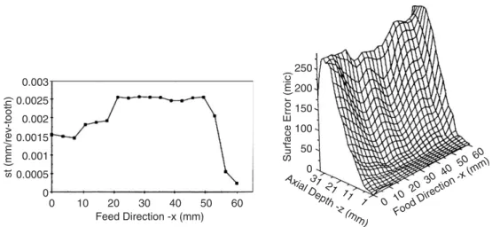
The same plate presented in Section 3.4 was machined using the scheduled feed rate for the allowable form error of 250mm. The scheduled feed rates used in the test and the measured resulting form errors are shown inFig. 8. Again, the ﬂexible force model was used in the simulations. The ﬁgure also shows that the form errors are kept within the tolerance using the scheduled feed rates.

4.3.2. Milling conditions for minimal form error

Up milling experiments were performed on free machin-ing steel by usmachin-ing a 19 mm diameter carbide end mill with 301 _{helix and 50 mm gauge length to demonstrate the} optimal selection of cutting conditions. The work piece was rigid and the form errors were only due to tool deﬂections. Axial depth of cut was 19 mm in all tests. The linear tool clamping stiffness was measured to be 25 kN/mm. Cutting force coefﬁcients were calibrated as: KT¼1140ðMPaÞ,

KR¼0:470,p¼0:28,q¼0:078. The maximum from error

and SMSE were simulated for a range of radial depths and feed rates, and the results indicate that the optimal radial depth is close to 3.3 mm[7]. In order to verify these results, several milling tests were performed with different radial depths and feeds which are shown in Fig. 9. The ﬁgure shows that there is a very good agreement between experimental and simulations results, and the form error is minimal for radial depth of about 3.35 mm. Compared to 1 mm radial depth, the MRR is more than tripled even though the form errors are almost the same. In addition, at 3.35 radial depth, the feed rate can be increased without

(10)

affecting the form errors, which further increases the MRR signiﬁcantly.

5. Conclusions

In this paper, analytical milling force, part and tool deflection, and form error models are presented, and their application in improving the performance of the process is demonstrated. The milling process is considered due to its complex geometry and mechanics, however similar model-ing methodology can be applied to other machinmodel-ing processes such as turning. On the other hand, the models can be extended to more complex milling processes such as ball end and five-axis milling. These models provide general information about the relations between the process performance and the process parameters. In addition, they can be used to simulate real cases, and the best set of parameters to improve the process performance can be selected. It should be noted that the process optimization can only be done on a stable process as demonstrated in [24]. Thus, the chatter suppression methods are presented in the second part of the paper [25]must be applied first.

For very practical and fast implementation of these models in industry, however, interfaces between CAD/CAM systems and/or CNC codes have to be developed ﬁrst.

References

[1] M.E. Merchant, Basic mechanics of the metal cutting process, ASME Journal of Applied Mechanics 66 (1944) 168–175.

[2] M.E. Martelotti, An analysis of the milling process, Transaction of the ASME 63 (1941) 677–700.

[3] F. Koenigsberger, A.J.P. Sabberwal, An investigation into the cutting force pulsations during milling operations, International Journal of Machine Tool Design and Research 1 (1961) 15–33.

[4] W.A. Kline, R.E. DeVor, I.A. Shareef, The prediction of surface accuracy in end milling, Transactions of the ASME Journal of Engineering for Industry 104 (3) (1982) 272–278.

[5] W.A. Kline, R.E. DeVor, I.A. Shareef, The effect of run out on cutting geometry and forces in end milling, International Journal of Machine Tool Design and Research 23 (1983) 123–140.

[6] J.W. Sutherland, R.E. DeVor, An improved method for cutting force and surface error prediction in ﬂexible end milling systems, Transactions of the ASME Journal of Engineering for Industry 108 (1986) 269–279.

[7] E. Budak, Y. Altintas, Peripheral milling conditions for improved dimensional accuracy, International Journal of Machine Tool Design and Research 34/7 (1994) 907–918.

[8] E. Budak, Y. Altintas, Modeling and avoidance of static deforma-tions in peripheral milling of plates, International Journal of Machine Tool Design and Research 35 (3) (1995) 459–476.

[9] E.J.A. Armarego, R.C. Whitﬁeld, Computer based modeling of popular machining operations for force and power predictions, Annals of the CIRP 34 (1985) 65–69.

[10] E. Budak, Y. Altintas, E.J.A. Armarego, Prediction of milling force coefﬁcients from orthogonal cutting data, Transactions of the ASME Journal of Manufacturing Science and Engineering 118 (1996) 216–224.

[11] Y. Altintas, P. Lee, A general mechanics and dynamics model for helical end mills, Annals of the CIRP 45 (1996) 59–64.

[12] Y. Altintas, S. Engin, Generalized modeling of mechanics and dynamics of milling cutters, Annals of the CIRP 50 (2001) 25–30. [13] E. Ozturk, E. Budak, Modeling of 5-axis milling forces, in:

Proceedings of the Eighth CIRP International Workshop on Modeling of Machining Operations, Chemnitz, May 10–11, 2005, pp. 319–326. 0.003 0.0025 0.0015 st (mm/rev-tooth) 0.0005 0 0 10 20 30 40 50 Feed Direction -x (mm) 60 0.002

0.001 _{Surface Error (mic)} 0 50 100 150 200 250 31 21 11 Axial Depth -z (mm) 1 60 50 40 30 20 10 0 Food Direction -x (mm)

Fig. 8. Form errors measured on the plate after it is machined with the scheduled feeds shown.

250 200 150 100 50 Experiment Simulation ft=0.1 mm/tooth ft=0.05 ft=0.1 0 0 1 2 3 4 5 6 7 8 9 Radial Depth of Cut (mm)

|Max. Surface Error

| (mic)

Fig. 9. Measured and predicted maximum form errors for different radial depths and feed rates.

(11)

[14] E. Budak, The mechanics and dynamics of milling thin-walled structures, Ph.D. Dissertation, University of British Columbia, 1994. [15] Y. Altintas, Manufacturing Automation, Cambridge University

Press, Cambridge, 2000.

[16] E.J.A. Armarego, R.H. Brown, The Machining of Metals, Prentice-Hall, Englewood Cliffs, NJ, 1969.

[17] G.V. Stabler, Fundamental geometry of cutting tools, Proceedings of the Institution of Mechanical Engineers (1951) 14–26.

[18] E. Kivanc, E. Budak, Structural modeling of end mills for form error and stability analysis, International Journal of Machine Tools and Manufacture 44 (11) (2004) 1151–1161.

[19] L. Kops, D.T. Vo, Determination of the equivalent diameter of an end mill based on its compliance, Annals of the CIRP 39 (1990) 93–96. [20] F. Beer, E. Johnston, Mechanics of Materials, McGraw-Hill, U.K,

1992.

[21] J.A. Nemes, S. Asamoah-Attiah, E. Budak, Cutting load capacity of end mills with complex geometry, Annals of the CIRP 50 (2001) 65–68.

[22] E. Rivin, Stiffness and Damping in Mechanical Design, Marcel Dekker, New York, 1999.

[23] E. Budak, Y. Altintas, Flexible milling force model for improved surface error predictions, in: Proceedings of the ASME 1992 European Joint Conference on Engineering Systems Design and Analysis, Istanbul, Turkey, ASME PD-47-1, 1992, pp. 84–94. [24] E. Budak, Improvement of productivity and part quality in milling of

titanium based impellers by chatter suppression and force control, Annals of the CIRP 49 (1) (2000) 31–36.

[25] E. Budak, Analytical models for high performance milling, Part II: process dynamics and stability, International Journal of Machine Tools and Manufacture, in press.