Simple Solutions for Compressed Execution in Vectorized Database System

University of Warsaw

Faculty of Mathematics, Computer Science and Mechanics

Vrije Universiteit Amsterdam

Faculty of Sciences

Alicja Luszczak

Student no. 248265(UW), 2128020(VU)

Simple Solutions

for Compressed Execution

in Vectorized Database System

Master thesis in COMPUTER SCIENCE Supervisor: Marcin ˙Zukowski VectorWise B.V. First reader: Peter Boncz

Vrije Universiteit Amsterdam Centrum Wiskunde & Informatica Second reader:

Jacopo Urbani

Vrije Universiteit Amsterdam

Supervisor’s statement

Hereby I confirm that the present thesis was prepared under my supervision and that it fulfils the requirements for the degree of Master of Computer Science.

Date Supervisor’s signature

Author’s statement

Hereby I declare that the present thesis was prepared by me and none of its contents was obtained by means that are against the law. The thesis has never before been a subject of any procedure of obtaining an academic degree. Moreover, I declare that the present version of the thesis is identical to the attached electronic version.

Abstract

Compressed execution is a method of operating directly on compressed data to improve database management system performance. Unfortunately, previously proposed techniques for compressed execution required major modifications of database engine and were diffi-cult to introduce into a DBMS. In this master thesis we look for solutions that are easier to implement, unintrusive and well suited to the architecture of VectorWise. We intro-duce an optimization based on RLE-compressed execution that consists of constant vectors

and primitive swapping mechanism. We also investigate possible benefits of operating on dictionary-encoded data and proposeon-the-fly dictionaries — a solution for providing uni-form domain-wide encoding while avoiding concurrency issues. The conducted experiments show a considerable potential of proposed techniques.

Keywords

database management systems, compression, compressed execution, query processing, database performance

Thesis domain (Socrates-Erasmus subject area codes)

11.3 Informatics, Computer Science

Subject classification

H. Software

H.2 DATABASE MANAGEMENT H.2.4 Systems

Contents

2.2.2. CPU cost of decompression . . . 11

2.2.3. Compression in column stores . . . 12

2.3. VectorWise architecture . . . 12 2.3.1. Execution model . . . 13 2.3.2. Compression in VectorWise . . . 15 2.4. Compressed Execution . . . 15 2.4.1. Early research . . . 16 2.4.2. Avoiding decompression . . . 16

2.4.3. Simultaneous predicate evaluation . . . 17

2.4.4. Code explosion problem . . . 18

2.4.5. Compression techniques . . . 18

2.5. Compressed execution in context of VectorWise . . . 19

2.6. Summary . . . 20

3. Run-Length Encoding . . . 21

3.1. Challenges of RLE-compressed execution . . . 21

3.1.1. Achieving compatibility with original code . . . 21

3.1.2. Increase in amount of code . . . 21

3.1.3. Selection vectors . . . 22

3.1.4. Variation in data clustering . . . 22

3.2. Proposed solution . . . 22

3.2.1. Detecting constant vectors . . . 23

3.2.2. Changes in expressions . . . 23

3.2.3. Impact on operators . . . 25

3.3. Experiments . . . 26

3.3.1. About the benchmark . . . 26

3.3.3. Detecting constant string vectors . . . 34

3.3.4. Filling vectors with constant value . . . 36

3.3.5. Conclusions from the experiments . . . 38

3.4. Impact of the vector size . . . 39

3.4.1. Effect on query execution performance . . . 39

3.4.2. Choosing the right vector size . . . 40

3.4.3. Variable vector size . . . 41

3.4.4. Vector borders problem . . . 41

3.4.5. Optimization algorithm . . . 42

3.5. Summary . . . 44

4. Dictionary Encoding . . . 45

4.1. Operations on dictionary-encoded data . . . 45

4.2. Global dictionaries . . . 47

4.3. The potential of dictionary compression . . . 47

4.3.1. On-Time benchmark . . . 48

4.3.2. TPC-H benchmark . . . 53

4.4. On-the-fly dictionaries . . . 57

4.5. Summary . . . 61

Chapter 1

Introduction

Database management systems provide functionality to safely store and efficiently operate on data to application developers. They are in use since 1960s and over time have become highly advanced and specialized software. Many data models, query languages and architectures were designed and implemented to achieve best possible performance in different workloads. Compression has been employed in database systems for years, both in order to save storage space, and to improve performance. The typical approach is to decompress all the data before it is passed to the query execution layer. This way, all the knowledge about data compression can be encapsulated within the storage layer making the implementation of the database system easier. This way however any opportunity for compressed execution is wasted.

Although the idea of compressed execution was first introduced in 1991 [GS91] and was shown to create a considerable potential of performance gains, there has been relatively little research in this area. The few proposed solutions required redesign and major adaptation of the database engine [AMF06], which made them poorly suited for integrating in existing database systems. None of them fitted the architecture of VectorWise [Zuk09], a DBMS that we focus on in this project.

We decided to try to answer the following question: Is it possible to introduce compressed execution in VectorWise, and achieve significant performance improvements, while avoiding any intrusive changes in the database engine?

Our goal was to propose new solutions, that would avoid or overcome difficulties of pre-vious ones, but not necessarily to implement all of them. We did not intend to make these solutions suitable for generic database systems, but instead we tried to tailor them to match the specific architecture of VectorWise. They are supposed to be non-invasive and straight-forward, and we consider simplicity an advantage. We aimed to achieve a notable part of possible performance benefits, but not to exploit every drop of opportunity at the price of introducing significant extra complexity.

The main contributions of this thesis are:

• proposing a simplification of RLE-compressed execution that consist ofconstant vectors

and primitive swapping mechanism, and evaluating its performance,

• estimating the benefits of using global dictionaries, and introducing the idea of on-the-fly dictionaries, that can provide similar gains, but are easier to maintain.

Not every compression technique exposes properties of data that can be used to execute queries more efficiently, but some of them do. Our work proves that these opportunities are well worth chasing. We show that it is often possible to get significant benefits by using

simple optimizations, which require just a fraction of effort that would have to be invested in order to implement full-blown compressed execution.

The reminder of this thesis is organized as follows. Chapter 2 provides basic introduction to database systems and explains how they employ compression to improve performance. It also presents the notion of compressed execution and reviews related work. Next, in Chapter 3 we discuss RLE-compressed execution, show the challenges it poses, and explain how they can be avoided with constant vectors. We provide benchmarking results for this solution. Chapter 4 explores the topic of operating on dictionary-compressed values, evaluates the benefits and discusses the problems of maintaining uniform encoding for entire columns or domains. Then we propose a possible solution of those problems called on-the-fly dictionaries. Finally, we present conclusions of this thesis and discuss future work in Chapter 5.

Chapter 2

Preliminaries

This chapter is intended to familiarize the reader with basic concepts that will be referred throughout this thesis. These include database management systems, compression and com-pressed execution, as well as the architecture of VectorWise.

First, we provide an overview of the basic aspects of database systems in Section 2.1. Section 2.2 discusses the role of compression in databases and introduces a number of com-pression schemes. The description of VectorWise database system is provided in Section 2.3. Section 2.4 presents the idea of compressed execution. Finally, in Section 2.5 we examine the usability of different approaches to compressed execution in context of VectorWise.

2.1. Database introduction

A database management system (DBMS) is a software package that allows applications to store and access data in a reliable and convenient way. The application developers do not have to implement specialized data manipulation procedures, but instead depend on functionality provided by DBMS. A database system accepts the description of the task expressed in a high-level language, decides how it should be performed and returns the results to the application.

The modern DBMSes are very specialized software and provide a number of advanced features, for example, they analyse many possible ways of completing a given task to choose the most effective one (query optimization), create backup copies, enforce data integrity, allow many users to modify the data in parallel while avoiding concurrency issues, and prevent unauthorized access.

2.1.1. Relational model

The data model determines the way that database is organised and operations that can be performed on data. Many different approaches were proposed over the years (e.g. hierarchical, object-oriented, XML, RDF), but therelational model remains the most widespread.

In the relational model the data is divided into relations. A relation has a number of

attributes. Each attribute has a corresponding domain, i.e. a set of valid values. A relation is an unordered set of tuples. A tuple contains exactly one value for each of the attributes of appropriate relation. A relation is traditionally depicted as a table, where columns rep-resent different attributes and rows correspond to tuples (see an example on the left side of Figure 2.3).

Client application client query result query DBMS (SQL) client query Client application MAL generator (SQL) frontend SQL formatted results relational plan SQL interface results MAL optimizers optimized MAL query processing requests results MonetDB

Data processing operators

GDK requests data data MAL query data requests Query rewriter Query parser parse tree data Query optimizer Query executor

Buffer manager / storage

normalized form

optimized query MAL interpreter

Figure 2.1: Architecture of a database management system (from [Zuk09]).

them operators. Some examples are: selection, projection, join, union, Cartesian product. We will not discuss them here. However, we will describe their physical counterparts in VectorWise in Section 2.3.1 and in Section 2.1.3 we will explain how operators interact with each other in the iterator model.

2.1.2. DBMS architecture

Although different database systems have different components, in general they follow a multi-layer architecture presented in Figure 2.1. We will now explain the role of each of these multi-layers. First, the client application has to describe the task that it wants to be performed. Such a task is called aquery and it is expressed in a special language, e.g., SQL. The query is then passed to the database system.

The query parser analyses the query. If the syntax is correct, the parser will produce an internal representation of the query, calledparse tree.

Next, the query rewriter ensures that the parse tree has correct semantics. It checks whenever the accessed attributes actually exist in proper relations, operations are performed on correct data types, and so on. The result is a tree innormalized form, specific for a given database system, and usually similar to relational algebra.

Then, the query optimizer tries to find the most efficient way of executing the query. It analyses many possibilities and modifies the tree according to its decisions. If an operator has many physical equivalents, the query optimizer has to pick the most suitable implemen-tation.

Thequery executor is the part of database system which performs the actual query pro-cessing. It requests the data from the storage layer and operates on it according to the query plan provided by the query optimizer.

Finally, the buffer manager or the storage layer is responsible for managing in-memory buffers as well as accessing and storing the data on disks or other media.

Project Bonus = (Age − 30) * 50 Select Age > 30 Scan People Id, Name, Age,

User tuple tuple tuple next() next() next()

Figure 2.2: Example of an operator tree (from [Zuk09]).

2.1.3. Operator trees

We will now discusstuple-at-a-time iterator model, which is the most popular way of imple-menting a database engine. The VectorWise engine also evolved from this model.

In the iterator model, the physical plan produced by a query optimizer consists of a num-ber of operators. These operators are objects corresponding to relational algebra operators. Each of these objects implements the methods open(), next() and close(). They are organized in the operator tree, so that the result of the root operator is the result of the entire query.

The open() method initializes the operator. When next() is called, the operator produces and returns the next tuple. Theclose()method is used when the query execution is terminated to free the resources. All of those methods are called recursively on children operators.

An example operator tree for a query

SELECT Id, Name, Age, (Age - 30) * 50 AS Bonus FROM People WHERE Age > 30

is presented in Figure 2.2. We will now describe how this query is executed.

First, the Project operator is asked for the next tuple. Project requests a tuple from the Select operator, and Select operator request a tuple from Scan. The Scan operator reads the next tuple from the table and passes it back to Select. Select uses this tuple to evaluate its condition. If the tuple fails to meet the condition, then Select asks Scan for the next one. Otherwise, the tuple is returned to Project. Project creates a new tuple with copies of Id, Name and Age attribute values, and the computed Bonus. The new tuple is then passed to the user and the process is repeated. When the Scan operator detects that there are no tuples left to read, it returns a special value that marks the end of tuple stream.

2.1.4. Storage organisation

Choosing the database model and the execution model does not determine the organisation of physical database representation, that is, the way the data is stored on persistent media.

Relation NSM representation DSM representation 101 Alice 22 102 Ivan 37 104 Peggy 45 105 Victor 25 108 Eve 19 109 Walter 31 112 Trudy 27 113 Bob Zoe 42 115 Charlie 35 114 29 Id 101 115 114 113 112 109 108 105 104 102 Name Ivan Peggy Victor Eve Walter Trudy Bob Zoe Charlie Alice 22 37 45 25 19 31 27 29 42 35 Age 101 115 114 113 112 109 108 105 104 102 Ivan Peggy Victor Eve Walter Trudy Bob Zoe Charlie Alice 22 37 45 25 19 31 27 29 42 35 Page 2

Page 1 Id Name Age

Figure 2.3: Example of a relation and its NSM and DSM representations (from [Zuk09]).

The most popular method is to store the tuples of a given relation one after another in continuous manner. This approach is called N-ary storage model (NSM) and database systems employing it are calledrow stores. It is depicted in the middle part of Figure 2.3.

An alternative method is to store values of each attribute separately. It is called decom-posed storage model (DSM) and DBMSes using it arecolumn stores. The same relation stored in DSM is shown in the right part of Figure 2.3.

Both of these solutions have their advantages and shortcomings. Their performance differs greatly depending on the workload and characteristics of the used database engine [ZNB08, AMH08]. There are also mixed approaches that try to get the best of both worlds. For example, PAX [ADHS01] stores values of different attributes separately, but it never splits a single tuple between two or more blocks. VectorWise allows both column-wise and PAX storage.

2.1.5. Database workload

Database systems were initially intended mostly foron-line transactional processing (OLTP) applications. They were designed to cope with many concurrent reads and updates, with each query accessing a relatively small number of tuples. The main goal was to minimize the portion of the data that has to be locked in order to modify a tuple [MF04]. Example queries from an OLTP workload include recording a bank transaction or checking price of a product. TPC-C benchmark [TPC10] is a standard tool for comparing performance of different database systems in OLTP applications.

On-line analytical processing (OLAP),data-mining and decision support system provide an entirely different workload. The queries usually only use a few attributes, but may access a large portion of tuples. The example is computing the fraction of computer games sold to persons that are 50 or older. The most widespread OLAP benchmark is TPC-H [TPC11].

The database systems optimized for different workloads have to be designed differently to achieve best performance. The DBMSes intended for OLTP queries are typically row stores following the tuple-at-a-time iterative model. The ones intended for analytical workloads are more often column stores. They sometimes employ an alternative query execution model, for example, vectorized execution as described in Section 2.3.1.

2.2. Compression in databases

Database systems often store data in compressed form. Compression can be applied to persistent data — that is, to the actual content of a database — as well as to intermediate results of query processing.

It is widely known that compression can improve the performance of a database systems [AMF06, Aba08, GS91, RHS95, Che02]. First, the time required to transfer the data from disk to main memory is shorter because the amount of data that has to be transferred is reduced. The same applies to moving data from main memory to CPU cache (the topic of in-cache decompression was explored in [ZHNB06]). Second, a bigger fraction of database can fit in the buffer pool, so the buffer hit rate is higher. Third, data can be stored closer together, which can be beneficial when using magnetic disks because it helps to reduce seek times.

However, these advantages come at the price of decompression overhead. We will explore this topic in Section 2.2.2.

2.2.1. Compression schemes

Database systems have special requirements for the compression methods rarely met by general purpose compression schemes. For that reason many compression algorithms were designed specially for database use [ZHNB06, GRS98, RHS95, HRSD07, RH93].1

One of the requirements is allowingfine-grained access to the data, which means that in order to read just few values we don’t have to decompress the entire page, but only a small fragment of it. The smaller that fragment is, the better. For example, when using dictionary or frame of reference encoding (described below), we don’t have to decompress any excessive data. Contrary, when using an adaptive scheme — one where the encoding is constructed basing on previously compressed or decompressed data, e.g., LZW – the decompression of the entire page is unavoidable. Providing fine-grained access to data is an important property that plays a major role in designing a compression scheme for database use [ZHNB06, GRS98, RHS95].

We will now present short descriptions of a number of compression schemes used in database systems. For more details we refer to [RH93, Aba08].

Fixed-width dictionary encoding In dictionary encoding we map values to fixed-width

codes. A data structure for translating codes into values and values into codes is called a dic-tionary. An example of compressing data using dictionary encoding is shown on Figure 2.4. This compression scheme requires knowing the number of distinct values upfront, before the compression process can begin. In practice, we have to use two-pass method: in the first pass we count distinct values and build a dictionary, and in the second pass we compress the data.

Dictionary encoding achieves a very high decompression speed, but it’s compression ratio can be ruined by outliers — values that occur extremely rarely in the input, but still have to included in the dictionary. A solution for this issue can be found for example in [ZHNB06].

1

Compression algorithms designed for DBMS use — unlike general purpose compression methods — can exploit the fact that data in a database has specific types (e.g. decimals, strings, dates). This allows better compression ratios (defined as the ratio between the compressed data size and the original data size) and lower CPU usage during decompression.

input dictionary (2 bits) encoded output ABACDAB −→ A 00 B 01 C 10 D 11 −→ 00 01 00 10 11 00 01

Figure 2.4: Example of dictionary encoding.

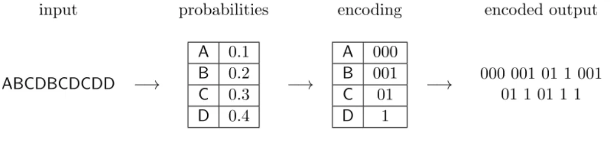
Huffman encoding Huffman encoding replaces occurrences of values with codes, just like

the dictionary encoding. However, the lengths of codes are variable. The values that occur often get shorter codes, and the values that occur rarely get longer ones. To ensure no ambiguity during decompression, no code is a prefix of another one.

Just like with dictionary encoding, we first have to determine the encoding before we can start compressing data. If statistics are not available upfront, we have to examine the data and determine probabilities of occurrence of different values. The actual algorithm for deriving codes from probabilities can be found in [Huf52]. An example of Huffman-encoded data is presented on Figure 2.5.

input probabilities encoding encoded output

ABCDBCDCDD −→ A 0.1 B 0.2 C 0.3 D 0.4 −→ A 000 B 001 C 01 D 1 −→ 000 001 01 1 001 01 1 01 1 1

Figure 2.5: Example of Huffman encoding.

Huffman encoding results in better compression ratios than dictionary encoding, but it is also slower to decompress, because we first have to determine the length of the code. This problem was addressed for example in [HRSD07].

Run-length encoding The run-length encoding replaces sequences of identical values by

a pair: a value and the number of its repetitions. Such a group of equal consecutive vales is called a run. The groups of values that cannot be effectively compressed using RLE are marked with negative run length. An example of RLE compression is shown on Figure 2.6.

input encoded output

AAAAAABBBCCCCCCC

EEEABCDEDDDDDDDD −→

6:A3:B7:C 3:E

−5:ABCDE 8:D

Figure 2.6: Example of run-length encoding.

RLE is useful for columns that contain long runs. This is typical for ones that data is sorted on or ones that contain repeated zeroes or nulls.

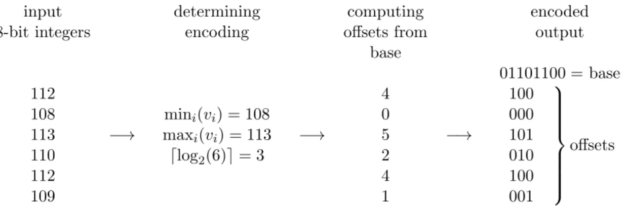
Frame of reference (prefix compression) FOR is a method for compressing numeric data. To encode values v1, v2, . . . , vn, it first finds the minimum and maximum value. It

records mini(vi) followed by vk−mini(vi) for k = 1,2, . . . , n. Each of those differences is

encoded using dlog₂(maxi(vi)−mini(vi) + 1)e bits [ZHNB06]. An example in presented in

Figure 2.7.

input determining computing encoded

8-bit integers encoding offsets from output

base 112 108 113 110 112 109 −→ mini(vi) = 108 maxi(vi) = 113 dlog₂(6)e= 3 −→ 4 0 5 2 4 1 −→ 01101100 = base 100 000 101 010 100 001                offsets

Figure 2.7: Example of frame of reference compression.

2.2.2. CPU cost of decompression

In the recent years we observed a growing disparity between the performance of disks and CPUs [BMK99, Che02, ZHNB06]: the available processing power grows at much faster rate than the disk bandwidth. The advent of multicore processors makes this disproportion even stronger. As a consequence, database systems often have to be deployed on machines with RAID storage constructed of tens or hundreds of disks in order to provide the required I/O bandwidth [ZHNB06].

However, the issue of insufficient I/O bandwidth can be to some extent mitigated by applying proper compression schemes. We will explain this idea using a model proposed in [ZHNB06].

LetB denote I/O bandwidth,Q— query bandwidth (that is, the maximal rate at which data could be processed, assuming that I/O is not a bottleneck), andR — resulting actual bandwidth. We have:

R= min(B, Q)

Now, assume that the data is compressed so that the proportion between size of raw data and size of compressed data isr >1, and let the decompression bandwidth be C. The data required for query execution can now be provided faster (the physical bandwidth is obviously unchanged, but the information density is greater):

Bc=Br

On the other hand, the additional CPU time is used for decompression. One can check that: Qc=

QC Q+C Finally, we can determine the resulting bandwidth.

Rc= min(Bc, Qc) = min

Br, QC Q+C

I/O bound queries If the query was I/O bound, then we have R=B < Q. Now, if the query is still I/O bound after applying compression, then we have

Rc=Br=Rr

In other words, the performance was improved by a factor ofr (usually more than threefold). On the other hand, if the query is now CPU bound, then we have:

Rc=

QC Q+C

We can’t clearly say if that’s better or worse performance than before. If the difference between Q and B was big and a light-weight compression scheme was used (that is, C is significantly larger than B), then the query will be executed faster. However, too expensive decompression will surely ruin the performance.

The bottom line is that if the decompression bandwidthC is much greater than the I/O bandwidthB, then we can expect shorter execution times of I/O bound queries. Researchers tried to exploit this effect in a number of studies, e.g., [HRSD07, GRS98, ZHNB06].

CPU bound queries We have

QC

Q+C < Q < B < Br So we can conclude that

Rc=

QC

Q+C < Q=R

Therefore, using compression will hurt the performance of I/O bound queries. However, with light-weight schemes this effect is much less severe that with heavy-weight ones.

2.2.3. Compression in column stores

Column stores are considered to create better opportunities for reaching high compression ratios [Che02], because they keep values of a single attribute close together. Such values are much more likely to expose regularities useful for compression than values of different attributes.

Unlike in row stores, the column stores omit reading from disk attributes that are not needed to execute a given query. This way the I/O traffic is limited to necessary data. Therefore it often happens that either queries are not I/O but CPU bound [MF04] or at least the difference between I/O and query bandwidth is not very high. For that reason, only light-weight decompression methods can be used in a column stores without hindering query execution performance.

2.3. VectorWise architecture

VectorWise [Ing] is a state-of-the-art database system [Zuk09] for analytical applications that employs a wide range of optimizations designed specifically to exploit capabilities of modern hardware. In this section we discuss its architecture, focusing on aspects most relevant for this thesis.

input vector 11 8 20 3

+

→

-sint col -sint val

→

result selection vector 1 3

-Figure 2.8: Example of selection vector produced by selection primitive. Elements of input vector are compared one by one with input constant. Resulting selection vector contains indices of elements smaller than 10.

2.3.1. Execution model

Vectors

VectorWise employs the vectorized execution model. Here, data is not passed in tuples like in query execution engines of most other database systems, but instead it is partitioned vertically intovectors. Each vector holds values of a single attribute from many consecutive tuples. The number of elements in each vector is fixed and is usually in range 100. . .10000. In the traditional tuple-at-a-time model, operators have to acquire tuples to process one by one. To get next input tuple, they have to call methodnext()of their children operators. Those function calls cannot be inlined, and may require preforming complex logic. As a result, tuple-at-a-time model suffers from high interpretation overhead, that can easily dominate query execution. In vectorized execution model, operations are always performed on all values in a vector at once. A single call of next() method produces not a single tuple, but a collection of vectors representing multiple tuples. Hence, the interpretation overhead is amortized over hundreds or thousands of values, and the queries are executed more efficiently [Zuk09].

Apart from the ordinary vectors, there is a special kind of vectors used to denote that part of tuples must not be used during operator evaluation (e.g. because they were eliminated by an underlying selection). These vectors are called selection vectors and hold offsets of elements that should be used. An example of how a selection vector is created is shown in Figure 2.8.

Primitives

The operations working directly on data stored in vectors are usually executed using primi-tives. Primitives are simple functions, that are easy to optimize for a compiler and achieve high performance on modern CPUs. They are designed to allow SIMDization (using special instructions simultaneously performing the same operation on multiple input values) and out-of-order execution (reordering instructions by the CPU to avoid being idle while the data is retrieved), and to efficiently use CPU cache.

Primitives are identified by signatures, which describe the performed operation and types of input and output. For example, the signaturemap add sint col sint val represents signed integer (sint) addition (map add) of a vector (col — column) and a constant (val – value). Such a primitive is implemented with code similar to this [Zuk09]:

int

{

for (int i = 0; i < n; i++)

result[i] = param1[i] + *param2;

return n; }

Expressions

Expressions are objects that are responsible for executing primitives. They bind a primitive to its arguments and provide a vector to store the results. Expressions are organized in a tree structure and they are evaluated recursively. Hence, the evaluation of an expression results in evaluation of its children expressions.

For example, in order to compute

x+y 1 +√z

where x, y and z are attributes of type dbl, we would have to construct following tree of expressions:

Expression with map / dbl col dbl col

Expression with map add dbl col dbl col

Column x

Column y

Expression with map add dbl val dbl col

Constant 1 Expression with map sqrt dbl col Column z Operators

As we explained earlier, query plans are composed of operators that loosely match the rela-tional algebra operators. They contain generic logic for performing different operations like joins or selections. Operators do not manipulate data directly, but instead use appropri-ate primitives, often wrapped in expressions. More information about this topic is available in [Zuk09].

The following list contains descriptions of VectorWise operators. It does not feature all of the operators, but only ones that are used later in this thesis.

• Scan is responsible for communicating with the storage layer to obtain table data required for query processing.

• Projectcan introduce new columns with values computed from input columns. It can also rename or remove columns.

• Aggr divides tuples into groups and compute statistical functions (max, min, sum, count) for each of the groups. We call it aggregation, the columns used for dividing tuples aregrouping columns orgroup-by columns, and the results of statistical functions are aggregates. Aggr can also be used for duplicate elimination.

• Sort returns exactly the same tuples as it consumes, but in different ordering, deter-mined by the values in sort columns.

• TopN also returns sorted tuples, but only firstN of them, while the rest is discarded.

• HashJoinprocesses two streams of tuples. It matches and returns pairs of tuples from different streams that have equal values inkey columns. For that purpose, it uses a hash table.

• CartProd also processes two streams of tuples, but returns all the possible combina-tions of pairs of tuples from different streams.

2.3.2. Compression in VectorWise

VectorWise is intended for analytical workloads, so it uses column-wise storage [Zuk09] (see Section 2.1.4). That is, it partitions data vertically and stores values of each attribute sepa-rately. As we explained, this creates much better opportunities for using compression effec-tively than the row-wise storage, because the data from the same domain and with similar distribution is stored near each other.

In VectorWise, compression is used to obtain better query execution performance, rather than to save storage space, but there is no notion of compressed execution. All the data is decompressed before passing it to the scan operator [ZHNB07].

Different parts of a single column may be compressed using different compression schemes. In VectorWise, the most appropriate scheme is chosen for each part automatically by analysing samples of data, and picking the scheme that offers best compression ratio. It is also possible to assign a fixed compression scheme to a column.

To match the vectorized execution model, the decompression process is performed with a granularity of a vector. Scan does not request the next tuple or value from the storage layer, but instead it asks for an entire vector. This way the decompression can be performed more effectively, because the overheads are amortized across a large number of values.

VectorWise employs a number of light-weight compression methods. Some of them were designed specifically to exploit the capabilities of super-scalar CPUs [ZHNB06].

2.4. Compressed Execution

The traditional approach to compression in database systems is to eagerly decompress all the data. The decompression may take place before the data is placed in I/O buffer (see Figure 2.9a), or before it is passed to processing layer (see Figure 2.9b). This way the execution engine can be kept completely oblivious of data compression, but also many optimization opportunities are wasted.

An alternative approach is to employ compressed execution, that is to allow passing the data from storage layer and between operators in compressed form. The decompression is then performed only when it’s needed to operate on data (see Figure 2.9c). This way the amount of memory required for query execution can be reduced, unnecessary decompression can be avoided and even some of the operations can be performed directly on compressed data. However, this method also creates its own new challenges.

decompression

Query executor

Buffer manager

disk

(a) before placing the data in disk buffers decompression --Query executor Buffer manager disk

(b) when passing the data to scan operator (current VectorWise [ZHNB07])

-- decompression

Query executor

Buffer manager

disk

(c) when required by query executor to op-erate on data (compressed execution)

Figure 2.9: Different stages at which decompression can be performed.

2.4.1. Early research

The idea of compressed execution was first proposed by Goetz Graefe and Leonard D. Shapiro in their work from 1991 [GS91]. They focused mainly on reducing the usage of memory space, because spilling data to disks during joins, aggregations and sorting was a major issue at the time. Hence, they proposed to delay the decompression as long as possible. We call this approach lazy decompression, as opposed to traditional eager decompression.

Graefe and Shapiro assumed that each value is encoded separately, and that a fixed encoding scheme is used for each domain. They pointed out that a number of operations can be performed directly on the values compressed this way. The codes can be used for equality checks, as join attributes, for duplicate elimination and as grouping attributes in aggregations. Moreover, when values have to be copied, for example during projections or materialization of join results, the decompression of values would even be harming, since it would increase the amount of data to copy.

We should notice that this work had a purely theoretical character. The authors did not implement the proposed solutions, but just made estimations based on a simple model taking into account the number of I/O operations.

2.4.2. Avoiding decompression

There were many studies that focused on delaying or avoiding decompression. Their authors did not aim to actually perform operations on compressed data, but rather to analyse when and how the data should be decompressed.

Westmann et al. proposed in [WKHM00] to modify the standard next() method, so that it returns not only a pointer to the tuple, but also a set of values from this tuple. This set would initially be empty, but whenever a value from a given tuple would be decompressed, it would be added to the set. This way no value would have to be decompressed twice.

Chen et al. in [CGK01] suggested to usetransient operators, that is, ones that internally work on decompressed values, but return compressed results. They argued that lazy decom-pression can lead to suboptimal execution times, since once the data gets decompressed, it

Predicate to evaluate A = 0 AND C=2

Placement of codes in a bank empty A B C

1 bit 2 bits 2 bits 3 bits

Translating constants into codes A dictionary[0] = 11 C dictionary[2] = 101

Resulting expression to evaluate (x BIT-AND 01100111) == 01100101

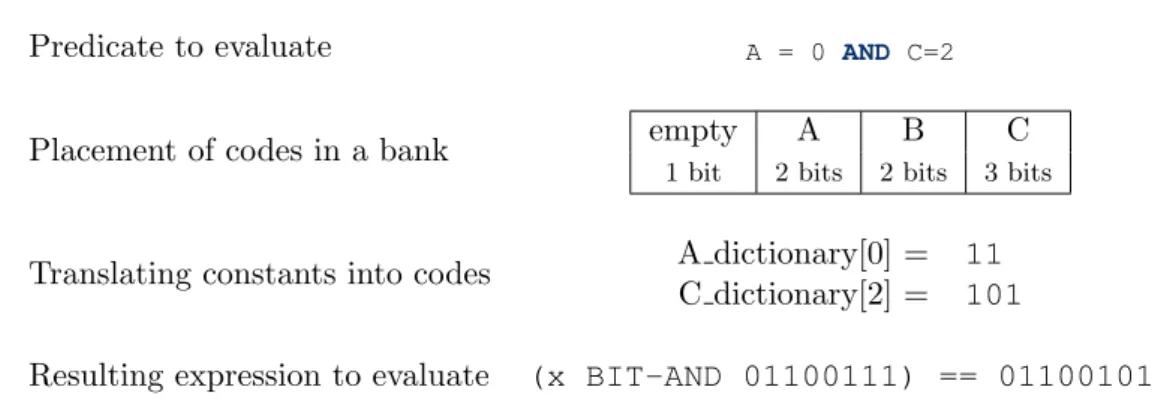
Figure 2.10: Example of converting conjuction of predicates into bit-wise operations on banks.

stays decompressed, which can increase the size of intermediate results and the number or required disk accesses for following operations like joins and sorting.

They also stressed the importance of taking compression into account while searching for the best query plan. The query optimizer should decide when to use eager, lazy or transient decompression, and adjust its estimates accordingly.

2.4.3. Simultaneous predicate evaluation

Johnson et al. argued in [JRSS08] that queries in decision support systems usually consist of an aggregation over a subset of tuples which have to meet tens of predicates. They give an example of aWHEREclause of a query from customer workload which illustrates this property:

WHERE A = a AND B = b AND C IN (c, d) AND D = 0

AND E = 0 AND F <= 11 AND G >= 2

AND H IN (e,f) AND (I IN (g,h) OR I > j)

AND { nine other clauses }

They pointed that efficient evaluation of those predicates is critical for query performance and proposed a method of compressed execution designed for that purpose.

Johnson et al. proposed to use an order-preserving dictionary encoding for all of the at-tributes. To make the compression more efficient, they partitioned the relations horizontally, and used a separate set of dictionaries for each of the partitions.

The codes were packed into 128-bit wide banks, each containing values from many columns. The banks for a given set of columns were stored one after another. In other words, this so-lution does not use row-wise or column-wise, but a special bank-wise storage.

Johnson et al. decided to translate the predicates on attributes to bit-wise operations on banks. A single CPU instruction operates on the entire bank, with many encoded attributes. This way a number of predicates can be evaluated in parallel. The translation rules are in general much too complicated to describe here, but we provide an example of one of the rules in Figure 2.10 to give the reader an idea of how such parallel evaluation can be executed.

Unfortunately, this approach is designed for a relatively small class of queries, and it is not clear whether it can perform well in more general workloads. Moreover, it implies very serious modifications in the execution and storage layer. It allows only a single compression scheme and needs a specialized bank-wise storage. Also, the series of operations on banks have to be compiled for each of the partitions separately.

2.4.4. Code explosion problem

Abadi et al. focused on integrating a number of compression schemes into a column store [AMF06]. They wanted to actually operate on the compressed data whenever possible, not just avoid the decompression. However, they observed that if no preventive steps are taken, then with each new compression technique the operators code will become more and more complex, since new special cases will have to be implemented for different combinations of compres-sion schemes in the input attributes. Also, they wanted to avoid exposing the details of compression to operators as much as possible.

To solve those problems, Abadi et al. decided to wrap the compressed data in special objects —compressed blocks— that would provide a uniform interface for accessing the data and its properties. This way the code of operators was not depending on implementation of individual compression schemes, but only on compressed blocks interface.

Abadi et al. proposed three Boolean properties of compressed blocks. TheisOneValue property was set, if all values in a given block were identical. TheisValueSorteddenoted that values in a given block were stored in a sorted order. The isPosContig was true, if the values formed a consecutive subset of a column. These three properties were used to decide on the optimal handling of data by an operator.

As an example, consider properties of RLE-compressed blocks, each containing a single run. All values in a run are identical, and equal values are naturally sorted, soisOneValue = TRUE and isValueSorted = TRUE. Moreover, each run is a continuous fragment of a column, hence isPosContig = TRUE.

Access to the data was possible through one of two functions: getValue()andasArray(). The first one transiently decompressed a value, and returned it together with its position in the table. The latter one decompressed all the values in a compressed block and returned them as an array.

2.4.5. Compression techniques

We will now discuss the compression methods chose for compressed execution.

• Definitely the most popular encoding scheme was dictionary encoding. It was used in all the above approaches because of ease of decompression and possibility of checking equality of values without decompression. If the encoding was order-preserving, the range comparisons were possible as well. The study of Abadi et al. recommends this scheme for all the attributes with anywhere between 50 and 50.000 values, that do not have runs that could be exploited by RLE.

• The RLE was considered by Abadi et al. the best choice for all the attributes that have runs of average length at least 4. A number of operations — comparisons, hash-ing, computing aggregates, duplicate elimination — could be performed once per run, instead of once per value. However, this scheme was useful only for column stores, because of difficult decompression in row stores.

• Abadi et al. pointed that bit-vector encoding is well suited for attributes with small number of distinct values that does not compress well with RLE. Similar to RLE, the bit-vector encoding provides groups of identical values. However, it is only useful if we accept processing values out of order.

• The Lempel-Ziv compression techniques were used as well, but the only benefit that can be achieved with them is by delayed decompression, because they do not expose any useful properties of data.

In addition, for some of the compression schemes special variants were designed, to make them more useful in compressed execution. For example, Holloway et al.proposed in [HRSD07] a method of reordering the nodes of Huffman tree, which allows range compar-isons without decompression.

2.5. Compressed execution in context of VectorWise

Our objective was to integrate compressed execution into the VectorWise DBMS. We wanted to achieve significant performance improvements, but also to avoid any major and invasive modifications of the database engine. We wished the changes to be as transparent and non-intrusive as possible, and likely to be implemented in a limited time. We focused on benefiting in the most common cases, rather than on chasing every bit of optimization opportunity. We reviewed the solutions for compressed execution described in previous section to determine if they can be successfully adapted to our needs. We summarize our observations below.

Chen et al. and Westmann et al. focused on lazy and transient decompression. However, the savings in decompression time are becoming less important with the advent of multi-core processors and growing available CPU power. The disk spills during joins or aggregations are problems of small concern in VectorWise, since these operations are usually executed within main memory. Moreover, the decompression in VectorWise is performed at the granularity of a vector, because decoding each value separately would introduce a significant overhead. Since it is relatively unlikely that no value in a vector will be used, a vectorized database system creates much fewer opportunities to avoid decompression. Hence, we do not anticipate any notable performance improvements to be achieved using these methods.

The solution proposed by Johnson et al., that is, simultaneous evaluation of predicates using banks, is not well suited for VectorWise. First of all, to employ it, the storage layer would have to be converted to store the data not column-wise, but bank-wise, which is a major modification to the DBMS. Second, it allows only dictionary compression and demands that encoding is fixed for horizontal partitions. This in not in line with the design of VectorWise storage layer, where each column is independent from the others. Most importantly, this approach only covers a very limited set of queries. VectorWise is intended for more general workloads, and turning to the bank-wise storage would most probably hurt the performance of other queries.

The approach presented by Abadi et al. poorly fits the architecture of VectorWise en-gine. Implementing it would require a major reengineering effort. It is also not clear how to make this solution compatible with vectorized execution model without hindering the perfor-mance. The compressed blocks may contain arbitrary number of values, while the operators in VectorWise expect identical number of values in each of the input vectors. Hence, the vectors would have to be represented by a collection of compressed blocks and some of the compressed blocks would have to be split between the vectors. Operating on such collections would introduce prohibitive overheads.

Moreover, Abadi et al. assumed that a large number of compression schemes would be used and focused on preventing code explosion. However, for most data distribution only a very small subset of compression algorithms provides optimal or close to optimal benefits. Our aim is not to employ as many compression techniques as possible, but to find and employ the ones that are really useful.

Our investigation suggests that compressed execution provides significant performance optimization potential, but the techniques proposed so far does not seem to fit the VectorWise system. For that reason, we decided to search for alternative methods. In the reminder of

this thesis we will describe techniques that achieve most of possible benefits, and at the same time are non-intrusive and easy to implement.

2.6. Summary

This chapter explained the concept and architecture of database management systems. We discussed the role of data compression in DBMSes and presented the idea of compressed execution. We also described the basic aspects of VectorWise — an analytical database system on which we decided to focus in this project. Then, previous research on compressed execution was reviewed in context of VectorWise. We concluded that none of solutions proposed so far fits well the architecture of this DBMS. Therefore, in order to integrate compressed execution in VectorWise and avoid major reengineering, we have to seek for new methods.

Chapter 3

Run-Length Encoding

Run-Length Encoding, described in Section 2.2.1, allows compressing sequences of repeating values. This encoding method was shown to be particularly useful for compressed execution purposes in previous research [AMF06].

In this section, we will discuss the difficulties of making a vectorized database engine capable of operating on RLE-compressed data. We will then propose a solution inspired by RLE, that allows achieving significant performance improvements while having a minimal impact on the database engine.

3.1. Challenges of RLE-compressed execution

Introducing execution on RLE-compressed vectors into a database engine is a task with many pitfalls. We will now describe some of the basic challenges that must be faced during this process.

3.1.1. Achieving compatibility with original code

The use of RLE-compressed data during query execution requires making the whole engine able to deal with a new data representation. Instead, one could try reusing existing code. This can be achieved by providing a function that converts an RLE-compressed vector into an ordinary one and then making sure that each operator or expression that cannot work directly on RLE-compressed data will use this function before accessing the content of a vector. Depending on how the database engine is actually implemented, the second part may or may not be a trivial task.

3.1.2. Increase in amount of code

In order to benefit from RLE-compressed execution, we have to extend the engine with new, RLE-aware code. The volume of code that has to be introduced can prove surprisingly large. For example, let us consider a simple function that subtracts two vectors (a primitive map - sint col sint col()). To make it RLE-aware, we have to provide four versions of this function: one operating on two ordinary vectors, one operating on two RLE-compressed vector, and two operating on one ordinary and one RLE-compressed vector. If we want to have a choice between producing a result that is either ordinary or RLE-compressed vector, the number of versions doubles.

The different variants can often be automatically generated, but nonetheless such an increase in the amount of code is undesired and should be avoided if possible.

3.1.3. Selection vectors

Selection vectors, described in Section 2.3.1, create a challenge for RLE-compressed execu-tion. Due to how the selection vectors are represented in VectorWise it cannot be determined in a constant time if at least one value in a given run is selected. Hence, without search-ing through the selection vector we cannot tell if computations for a given run should be performed at all.

For some operations this problem can be evaded by ignoring the selection vector. The computations are then performed for all runs, as if all values were selected. We call this method full computation.

Unfortunately, full computation is only suitable for a limited set of operations which cannot result in failures. For example, execution of primitive map == sint col sint col will always succeed, because comparing any two numbers will produce a valid result. On the other hand, many operations does not have this property. For example, full computation for primitivemap / sint col sint col may result in a ‘division by zero’ error.

3.1.4. Variation in data clustering

It may happen that some parts of a column are well suited for RLE-compression (identical values are clustered together), while others are not. Using RLE-compressed vectors to repre-sent data from the first ones can bring performance improvements, while using them for the latter ones will only create an additional overhead.

Therefore, we should allow a scan operator to produce a mix of ordinary and RLE-compressed vectors, depending on their content. As a result, each and every expression and operator must be capable of handling any sequence of different kinds of vectors. A proper implementation cannot be chosen upfront while building an operator tree — it has to be selected dynamically during query execution.

3.2. Proposed solution

Our objective was to keep part of the benefits of RLE-compressed execution while limiting the impact on a database engine, simplifying implementation and avoiding the challenges described above. The RLE-compressed execution achieves reduced CPU-cost by performing operations once per run — a group of consecutive equal values — instead of once per value, and we aimed to exploit the same mechanism.

We propose not to introduce a new data representation for fully RLE-compressed data. Instead we shall focus entirely on vectors that hold values that are all equal, i.e. vectors that consist of a single run. We will call them constant vectors. In order to denote this property, we only have to add a single Boolean flag to a vector data structure. However, unlike with RLE, even a constant vector will still have to contain all values in order to ensure that it can be safely used in the same way as all the other vectors.1

This approach makes it easier to overcome the challenges described before. The problem of code compatibility is evaded by using a single data representation. The original code will be oblivious to whether vectors are constant or not. These parts will not achieve any performance improvements, but at least will not lose correctness. The increase of amount of code can be limited by reusing code that is already a part of the system. This process is described in Section 3.2.2. The presence of selection vector is no longer a problem: in

1

This assumption is made to avoid engineering difficulties emerging due to how VectorWise was imple-mented. We will later show that it actually causes a significant overhead and discuss abandoning it.

a constant vector all values are equal, so it only mattershow many values are selected, but notwhich ones exactly. Finally, since there is no structural difference between constant and non-constant vectors, this method is not spoiled by variations in data clustering.

3.2.1. Detecting constant vectors

The scan operator should mark some of produced vectors as constant. It is not necessary to detect all of the constant vectors, as false negative may only harm performance, but not correctness. We should aim at marking as many as possible while keeping the CPU-cost low. Non-string attributes We first decided to only try to find constant vectors for data stored in RLE-compressed disk blocks. There are two reasons for this:

1. Checking if a vector is constant during RLE decompression is very cheap in terms of CPU-time, while the same is not true for other compression schemes in VectorWise. 2. For a column that can produce a significant fraction of constant vectors (i.e. has plenty

of very long runs) RLE is most probably the best suited compression scheme. Then columns for which a different compression scheme is better suited are less likely to give us a lot of constant vectors.

String attributes A workaround was required for string attributes, because there is

cur-rently no implementation of RLE-compression for strings in VectorWise.

We decided to manually check each vector produced by scan operator, i.e. compare its values one-by-one. This introduces a significant overhead, that is unacceptable in production code. However, this overhead is easy to accurately measure. It is also easy to avoid by implementing an appropriate compression scheme. Hence, we decided that this method can be used for the purpose of this thesis.

3.2.2. Changes in expressions

We will now discuss how to modify the expression object, so that it can seize the opportunities provided by constant vectors.

Primitives

As we explained in Section 2.3.1, expressions have an assigned primitive that they are re-sponsible for calling. Each kind of primitive comes in many variations, depending on what kind of arguments it is intended for. The arguments may be vectors (represented bycol in primitive’s signature) or constants (represented byval).

Primitive swapping

Let us notice that constant vectors can often be treated as if they were just a single value. For example, consider primitive map + dbl col dbl col. It can be intuitively written as:

for(i = 0; i < n; i++)

result[i] = param1[i] + param2[i];

Assume that the second argument is a constant vector. There is no need to actually read the content of this vector. Instead we can do:

for(i = 0; i < n; i++)

result[i] = param1[i] + *param2;

This approach should be beneficial, as it requires moving less data from memory to CPU registers and can improve cache utilisation.

The second listing is simply the map + dbl col dbl val primitive. Hence, a similar primitive — one that has a val instead of col in its name — can be called instead of the default one. The same idea can be applied to many different primitives.

We propose to choose the most appropriate primitives dynamically during query execu-tion. This decision should depend entirely on whenever argument vectors are constant or not. We call this process primitive swapping.

Implementation

In order to make primitive swapping possible, we have to modify the expression object. Those changes can be divided in two categories: those that come into effect when the operator tree is constructed, and those that come into effect whenever a primitive has to be executed.

• Build phase

During the construction of the operator tree, the expressions determine which primitives they should use. Normally they only choose one primitive, and use it during the whole query execution.

However, in our proposal they have to retrieve not only a single primitive, but also all the primitives that it can be swapped for. Determining which primitives should be selected is not difficult. After finding the default primitive, we can easily construct their names through simple string operations (substitutingcolforvalin the primitive name).

This process might be laborious, but it only takes place once per expression.

• Execute phase

Every time an expression is evaluated and a primitive has to be called, the argument vectors should be examined. Depending on whether any or all of those vectors are constant, an appropriate primitive has to be chosen: the morevals in the name (instead of cols) the better, but each new val must match an argument that is a constant vector.

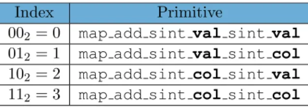
Making this decision has to introduce some additional interpretation overhead. How-ever, it can be effectively implemented. We propose to prepare a table with choices for all possible combinations of constant and non-constant argument vectors at build time. Each argument vector would correspond to one bit in table index. In order to choose the right primitive, we’d only have to iterate over all argument vectors and set a proper bit for every non-constant one. An example of this procedure is presented on Figure 3.1.

Caveats

The described approach allows us to ‘recycle’ code that is already a part of the system for compressed execution. However, it also has a certain disadvantage: the result type (a vector or a value) of a primitive is determined implicitly from the types of its arguments. This

(a) Table of primitive choices (created at build time):

Index Primitive

002= 0 map add sint val sint val

012= 1 map add sint val sint col

102= 2 map add sint col sint val

112= 3 map add sint col sint col

(b) Computing index (performed for each expression evaluation):

1 0

= 2

%

-is constant(param1) == FALSE is constant(param2) == TRUE

(c) Selected primitive:

102= 2 map add sint col sint val

Figure 3.1: Choosing best primitve in expression withmap add sint col sint col func-tion.

means that, for example, the result of the primitive map + dbl val dbl col is a vector, while the result of map + dbl val dbl valis just a single value.

We decided to keep an original data representation, and therefore each constant vector actually has to contain all those equal values. Hence, whenever swapping of primitives affects the result type (changing it from a vector to a value), we have to manually ‘fill’ the result vector with copies of value returned by a primitive. Luckily, those situations are easy to identify.

The necessity of ‘filling’ constant vectors introduces a significant overhead, but it does not make using constant vectors pointless. We will examine this overhead and explain how to remove it in Section 3.3.4.

The performance of constant vectors optimization strongly depends on choosing correct vector size for a given data. We will explain this problem in Section 3.4.

3.2.3. Impact on operators

We discussed the modifications of expressions needed to make them aware of constant vectors. Those changes alone can bring notable performance benefits. However, not all optimization opportunities of constant vectors can be exploited by altering only the way expressions are evaluated. While some operators — e.g. Project — can benefit fully from constant vectors without any changes to their code, others require some modifications.

As an example we will now examine the aggregation operator. The work of Aggr operator proceeds in two phases:

• and a produce phase when it outputs the results of the previous phase.

There are no opportunities to use constant vectors in the latter, so we will focus on the build phase.

The first step in the build phase is to divide the input into groups that refer to certain values of attributes from GROUP BYclause. Depending on the type of those attributes, this operation can be performed in one of two ways:

• Direct aggregation — the group number is computed arithmetically from the values of group-by attributes. This computation is performed using expressions, so it benefits from constant vectors without any modifications.

• Hash aggregation — the group number is determined using a hash table. First, the hash values for all group-by attributes are computed through a proper expression. Then a lookup-or-insert function working on a hash table is called. For constant vectors it is enough to perform this operation once for entire vector, instead of repeating it for each value in a vector. Therefore an additional ifstatement should be added to hash aggregation code.

The second and final step is updating the aggregates. Here primitives computing sum, mini-mum, maximini-mum, count, etc. are called. For this purpose expressions are used and constant vectors optimizations are applied automatically.

3.3. Experiments

3.3.1. About the benchmark

We decided to test the constant vector implementation against real-life data. We used records of USA domestic flights from October 1988 to August 2009 [Res11]. The data consisted of a single tableOntime with ca. 125 millions of rows.

We run a set of 10 queries, that we will refer to as On-Time benchmark. They were previously used to compare performance of different analytical DBMSs [Tka09, Ker10]. Ontime table

The Ontime table had 93 columns of various types, but only a small subset of them was used during the benchmark. Below we present the schema definition of Ontime table with unused columns omitted.

CREATE TABLE "Ontime" (

"Year" SMALLINT DEFAULT NULL, ...

"Month" TINYINT DEFAULT NULL, ...

"DayOfWeek" TINYINT DEFAULT NULL, ...

"Carrier" CHAR(2) DEFAULT NULL, ...

"Origin" CHAR(5) DEFAULT NULL, "OriginCityName" VARCHAR(100) DEFAULT NULL, ...

"DestCityName" VARCHAR(100) DEFAULT NULL, ...

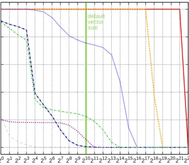
0 0.2 0.4 0.6 0.8 1 20 21222324 25 262728 29210211212213214215216217218219220221222

Fraction of values in runs of greater length

Run length default vector size Year Month DayOfWeek Carrier Origin, OriginCityName DestCityName DepDelay

Figure 3.2: The value runs in On-Time dataset.

... );

Value runs

We decided to investigate to what extent different columns of theOntimetable are suitable for RLE-compression. We examined lengths of value runs in each of them. The data was not sorted, but instead kept in the same order in which it was provided. The results are presented in Figure 3.2.

Since the data is naturally sorted on Year and Month, these two columns provide the longest runs of equal values. The scan operation on those columns should produce almost exclusively constant vectors. Therefore, we decided to use RLE-compression for Year and Month.

Carrier is a string column that consists of relatively long runs — 67% of all values are in runs of length at least 213. We can anticipate that a scan of Carrier will return a significant fraction of constant vectors if only the vector size is not greater than 212.

Finally,DestCityNamecould provide a bit more than 20% of constant vectors for vector size 210. The other columns do not create an opportunity to use our optimization.

Note that the plot lines forCarrierandDestCityNamehave middle sections that are notably less steep. It is a consequence of non-homogeneous data clustering in the dataset. All data is sorted onYearandMonth, but then within a single month it may be clustered in many ways. This results in dramatically different run lengths in parts of columns belonging to different months.

Column name Constant vectors Carrier 87.3–96.2% DayOfWeek 0.0% DepDelay 0.0% DestCityName 41.7% Month 99.8% Origin 1.0% OriginCityName 0.3% Year 99.9%

Table 3.1: Fraction of constant vectors produced during execution of On-Time queries. Note that these values differ from ones presented in Figure 3.2 due to non-homogenous data clus-tering.

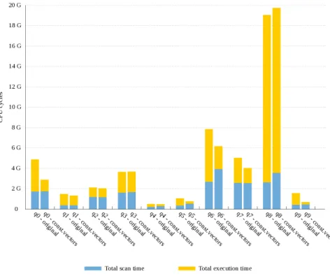
Figure 3.3: Execution times of queries from On-Time benchmark with and without constant vectors optimization.

3.3.2. Results

All test were executed on Intel(R) Quad Core CPU Q6600 @ 2.40GHz platform with 8 GB RAM. The reported results are mean times of query execution with hot disk buffers, i.e. no data had to be read from disk. We used the default vector size of 1024.

The results for entire benchmark are presented in Figures 3.3 and 3.4, as well as listed in Table 3.2. The queries and their operator trees are shown in Figures from 3.5 to 3.14. The fractions of constant vectors produced from each column while executing those queries are listed in Table 3.1. We will now discuss benchmark results in detail.

Figure 3.4: Execution times of queries from On-Time benchmark while using constant vectors compared to original VectorWise results.

Query Q0 Q1 Q2 Q3 Q4

Execution time:

– original 4869.6 1489.8 2106.2 3662.0 496.6

– with constant vectors 2884.5 1332.0 2051.5 3685.7 474.2

– change −40.7% −10.6% −2.6% +0.6% −4.5%

Query Q5 Q6 Q7 Q8 Q9

Execution time:

– original 1053.0 7838.3 5020.2 19049.9 1570.6

– with constant vectors 778.8 6213.2 4111.7 19813.0 723.9

– change −26.0% −20.7% −18.1% +4.0% −53.9%

Table 3.2: Execution times of queries from On-Time benchmark.

Query 0

The majority of query execution time is spent in direct aggregation Aggr1that usesYearand Month as group-by columns, and consumes ca. 125 millions of tuples. The use of constant vectors reduces the aggregation time by 65%.

As we described in Section 3.2.3, the direct aggregation consists of two steps: (a) comput-ing identifiers of groups to which each tuple belongs (throughmap directgrp*primitives), and (b) updating appropriate aggregates (throughaggr* primitives). The first part can be only slightly improved by use of constant vectors, because vector filling is necessary. However, the second part benefits greatly, because foraggr* primitives there is no such need.

WITH T AS ( SELECT Year, Month, COUNT_(*) AS C FROM Ontime GROUP BY Year, Month ) SELECT AVG(C) FROM T; Project Aggr2 Aggr1 Scan

Figure 3.5: Query 0 from On-Time benchmark and its operator tree.

SELECT DayOfWeek,

COUNT_(*) AS C

FROM Ontime

WHERE Year BETWEEN 2000 AND 2008

GROUP BY DayOfWeek ORDER BY C DESC; Sort Project Aggr Select2 Select1 Scan

Figure 3.6: Query 1 from On-Time benchmark and its operator tree.

SELECT DayOfWeek,

COUNT_(*) AS C

FROM Ontime

WHERE DepDelay > 10

AND Year BETWEEN 2000 AND 2008

GROUP BY DayOfWeek ORDER BY C DESC; Sort Project Aggr Select3 Select2 Select1 Scan

SELECT FIRST 10 Origin,

COUNT_(*) AS C

FROM Ontime

WHERE DepDelay > 10

AND Year BETWEEN 2000 AND 2008

GROUP BY Origin ORDER BY C DESC; TopN Project Aggr Select3 Select2 Select1 Scan

Figure 3.8: Query 3 from On-Time benchmark and its operator tree.

SELECT Carrier, COUNT_(*) FROM Ontime WHERE DepDelay > 10 AND Year = 2007 GROUP BY Carrier ORDER BY 2 DESC; Sort Project Aggr Select2 Select1 Scan

Figure 3.9: Query 4 from On-Time benchmark and its operator tree.

WITH T AS ( SELECT Carrier, COUNT_(*) AS C FROM Ontime WHERE DepDelay > 10 AND Year = 2007 GROUP BY Carrier ), T2 AS ( SELECT Carrier, COUNT_(*) AS C2 FROM Ontime WHERE Year = 2007 GROUP BY Carrier ) SELECT T.Carrier, C, C2, C*1000/C2 AS C3 FROM T JOIN T2 ON T.Carrier = T2.Carrier ORDER BY C3 DESC; Sort Project HashJoin Aggr1 Select2 Select1 Scan1 Aggr2 Select3 Scan2

WITH T AS (

SELECT Carrier,

COUNT_(*) AS C

FROM Ontime

WHERE DepDelay > 10

AND Year BETWEEN 2000 AND 2008

GROUP BY Carrier ), T2 AS ( SELECT Carrier, COUNT_(*) AS C2 FROM Ontime

WHERE Year BETWEEN 2000 AND 2008

GROUP BY Carrier ) SELECT T.Carrier, C, C2, C*1000/C2 AS C3 FROM T JOIN T2 ON T.Carrier = T2.Carrier ORDER BY C3 DESC; Sort Project HashJoin Aggr1 Select3 Select2 Select1 Scan1 Aggr2 Select5 Select4 Scan2

Figure 3.11: Query 6 from On-Time benchmark and its operator tree.

WITH T AS ( SELECT Year, COUNT_{(*) * 1000} AS C1 FROM Ontime WHERE DepDelay > 10 GROUP BY Year ), T2 AS ( SELECT Year, COUNT_(*) AS C2 FROM Ontime GROUP BY Year ) SELECT T.Year, C1/C2 FROM T JOIN T2 ON T.Year = T2.Year; Project HashJoin Aggr1 Select Scan1 Aggr2 Scan2

Figure 3.12: Query 7 from On-Time benchmark and its operator tree.

SELECT FIRST 10

DestCityName,

COUNT(DISTINCT OriginCityName)

FROM Ontime

WHERE Year BETWEEN 1990 AND 2000

GROUP BY DestCityName ORDER BY 2 DESC; TopN Project Aggr Select2 Select1 Scan