Modelling farm structural change A feasibility study for ex-post modelling utilizing FADN and FSS data in Germany and developing an ex-ante forecast module for the CAPRI farm type layer baseline

(1)

Modelling farm structural change

A feasibility study for ex-post modelling utilizing FADN and FSS

data in Germany and developing an ex-ante forecast module for the

CAPRI farm type layer baseline

Authors:

Alexander Gocht, Norbert Röder, Sebastian Neuenfeldt, Hugo Storm, Thomas Heckelei Editors:

María Espinosa, Sergio Gomez y Paloma 2 0 1 2

(2)

European Commission Joint Research Centre

Institute for Prospective Technological Studies

Contact information

Address: Edificio Expo. c/ Inca Garcilaso, 3. E-41092 Seville (Spain) E-mail: [email protected]

Tel.: +34 954 48 8458 Fax: +34 954 48 8434 http://ipts.jrc.ec.europa.eu/ http://www.jrc.ec.europa.eu/

This publication is a Scientific and Policy Report by the Joint Research Centre of the European Commission. Legal Notice

Neither the European Commission nor any person acting on behalf of the Commission is responsible for the use which might be made of this publication.

The opinions expressed are those of the authors only and should not be considered as representative of the European Commission's official position.

Europe Direct is a service to help you find answers to your questions about the European Union Freephone number (*): 00 800 6 7 8 9 10 11

(*) Certain mobile telephone operators do not allow access to 00 800 numbers or these calls may be billed. A great deal of additional information on the European Union is available on the Internet. It can be accessed through the Europa server http://europa.eu/.

JRC 75524 EUR 25555 EN

ISBN 978-92-79-27047-5 (pdf) ISSN 1831-9424 (online) doi:10.2791/17545

Luxembourg: Publications Office of the European Union, 2012 © European Union, 2012

Reproduction is authorised provided the source is acknowledged.

(3)

Acknowledgements

This study has been developed under the project "Modelling the effects of the CAP on farm structural change" (Contract 151949-2010-A08-DE). The project team would like to acknowledge the advice and assistance they have received from Maria Espinosa and Sergio Gomez y Paloma (DG JRC/IPTS). The results of the project were presented at the expert workshop in the Institute for Prospective and Technological Studies (IPTS) on the 7th/8th February 2011. We are indebted to the participants, in particular to Thierry Vard and Hubertus Gay (DG-AGRI) for their constructive and helpful comments and recommendations.

(4)

List of Tables

U

Table 1: U UCharacteristics of the different methodologies used in the out-of

sample predictionU 15

U

Table 2:U UDifferences between the FSS and FADN databases in GermanyU 17

U

Table 3:U ULength of time that farms remained in the German FADN sample

(1989-2008)U 18

U

Table 4:U UClassification of the FADN variables describing the farm structure to retrieve the 2-digit farm-classification and the CAPRI farm

classification for GermanyU 18

U

Table 5:U UDefinition of farm types considered for predictionU 19

U

Table 6:U UList of potential variables to be considered in an ex-post analysis

and the likely data sources on the EU levelU 24

U

Table 7:U UOverview of some key figures regarding the age information in the

German FADN sample (1989-2008)U 31

U

Table 8:U UTime-varying explanatory variables for the different farm types

selected in the Markov approachU 34

U

Table 9:U UVariables used in the MCI approachU 35

U

Table 10: U UOut-of-sample prediction fit measures for a fixed-effects panel

estimation and separate estimation per regionsU 50

U

Table 11:U UMean square error (MSE) and mean percentage deviation (pDev) of the out-of-sample prediction for different prediction methods

(averaged over all size classes)U 51

U

Table 12:U UFinal model specifications for the non-stationary Markov approach (in addition to the listed variables, regional dummy variables were

considered for all except one region in all models)U 52

U

Table 13:U UComparison of the Akaike Information Criterion (AIC) for different estimation methodsU 53

U

Table 14: U UMean square error (MSE) and mean percentage deviation (pDev) of the out-of-sample prediction for differentt prediction methods

(averaged over all size classes)U 53

U

Table 15: U UMean square error (MSE) and mean percentage deviation (pDev) of the out-of-sample prediction for the total number of farms for

(8)

U

Table 16:U UComparison of the in-sample prediction quality between a MCI approach and the benchmarka between 1989 and 2003 over a

four-year periodU 57

U

Table 17:U UImpact of a 10% increase in the respective variable on the number of farms per type compared with the reference scenario for the period of 2003-2007 (test set) based on the period 1989-2003

(training set)U 62

U

Table 18:U UImpact of a 10% decrease in the respective variable on the number of farms per type compared with the reference scenario for the period of 2003-2007 (test set) based on the period of 1989-2003

(training set)U 62

U

Table 19: U UEquations in the baseline estimationU 79

U

Table 20: U UAdditional equations for maintaining the ESU and type of farming

during estimationU 80

U

Table 21: U UNumber of holdings for DE93U 81

U

Table 22: U UPartial SGM shares, UAA and livestock density for all farm types

in the DE93 base yearU 82

U

Table 23: U UEvaluation of UAA for the different implementationsU 83

U

Table 24:U UEvaluation of ESU for the different implementationsU 84

U

Table 25: U UEvaluation of LU/UAA for the different implementationsU 85

U

Table 26:U UEvaluation of the partial SGM shares for the different

implementationsU 87

U

Table 27:U UIllustrative example calculating the distance between farm A and

three other farmsU 108

U

Table 28:U UIllustrative example calculating the distances between farms using

standardised Manhattan Block and Spherical DistanceU 109

U

Table 29: U UMatrix d for dimension Columns and Rows in CAPRI for farm type during baseline estimationU 118

U

Table 30: U UCalculation of the partial SGM in CAPRI Farm TypesU 119

U

Table 31: U UList of CAPRI files modifiedU 120

U

Table 32:U UNon-stationary Markov studies in the agricultural economics

literatureU 134

U

(9)

1B

List of Figures

U

Figure 1:U UComparison of the average (mean and median) annual changes in farm size (measured in € SGM) of German farms over time if the

farms’ activities are weighted with a constant or variable SGM.U 20

U

Figure 2:U UComparison of the average (mean and median) annual change in the farm specialisationa of German farms over time if the farms’

activities are weighted with a constant or variable SGM.U 21

U

Figure 3:U UDevelopment of the FADN-SGM per dairy cow in Upper Bavaria

(DE21) between 1986 and 2004.U 22

U

Figure 4:U UDevelopment of the average yield of wheat (dt/ha; SE110), maize (dt/ha; SE115) and milk equivalents (kg) per cow (SE115)

(averaged over all Germany FADN regions)U 27

U

Figure 5:U UOutput and input price indices for different farm productsU 28

U

Figure 6:U UAverage subsidies (€/year) received per farm

(West German FADN regions)U 29

U

Figure 7:U UShare of subsidies attributable to known sources for German FADN

farmsU 29

U

Figure 8:U UAverage land rent per ha (West German FADN regions)U 30

U

Figure 9:U UUnemployment rate of the civil dependent labour forceU 31

U

Figure 10:U UAverage summer temperature and slope for the different farm types in the German FADN regionsU 32

U

Figure 11:U URoot mean squared error (RMSE) between the predicted and the observed shares of the different types of farming across the region for different specifications of the MCI model (training set:

1989-2003; test set 2003-2007)U 58

U

Figure 12:U URoot mean squared error (RMSE) between the predicted and

observed shares of the different types of farming across the types of farming for different specifications of the MCI model (training set: 1989-2003; test set 2003-2007)U 59

U

Figure 13:U URoot mean squared error (RMSE) between the predicted and the observed shares of the different types of farming across the region for different specifications of the MCI model (training set:

1989-1999; test set 1999-2007)U 60

U

Figure 14:U UDependence of the root mean squared error (RMSE) on the number of FADN farms per region for the final set of the MCI model

(10)

U

Figure 15:U URoot mean squared error (RMSE) between the predicted and the observed shares of the different types of farming across the types of farming for the “final set” specification of the MCI model and a

“naive” estimation (training set: 1989-1999; test set 1999-2007)U 61

U

Figure 16: U UDistribution of the Steplength aggregated over four years for the

periods of 1999-2003 and 2003-2007 for FSS and FADNU 63

U

Figure 17:U UComparison of the change in the dominant specialisation of selected specialised farm types within 4-year intervals (average of

the two periods 1999-2003 and 2003-2007) for FSS and FADNU 64

U

Figure 18:U UMedian and average 4-year Steplength for the periods of 1999-2003 and 2003-2007 as a function of farm size for FSS and FADN farmsU 65

U

Figure 19:U UExample of the location of three farms (F1, F2 and F3) in a three

dimensional data spaceU 106

U

Figure 20:U UDevelopment of farm F1 from t = 1 to t = 6U 107

U

Figure 21:U UIllustrative example of two trajectories over 6 periodsU 107

U

Figure 22: U UDevelopment of the average step length per farm type (1-digit FADN typology) measured by the Manhattan-Block-Metrics

between 1995 and 2007U 110

U

Figure 23: U URelation of the one year to multi-year step length per farm type (1-digit FADN typology) measured by the

Manhattan-Block-MetricsU 111

U

Figure 24: U UDistribution of cumulated share of farms as a function of the annual step length for the different years (measured by Manhattan Block

distance)U 112

U

Figure 25: U UDistribution of cumulated share of farms as a function of the annual step length for the different farm types (measured by Manhattan

Block distance)U 113

U

Figure 26: U UDevelopment of the average annual change in the share of the

P1-P5 activity groups for the eight general farm types.U 114

U

Figure 27: U UNumber of farms and average development of farms regarding the share of P4 over 1 year in dependence of the initial share of P4 on

the total SGMU 115

U

Figure 28:U UNumber of farms and average development of farms regarding the share of P4 over 4 year in dependence of the initial share of P4 on

(11)

2B

Executive Summary

Study objectives

This study had the following specific objectives. The first objective was to review the existing methodologies for ex-ante and ex-post modelling of structural change. The second objective was to develop prototypes of analytical tools for ex-post and ex-ante analysis of structural change in agriculture based on FADN (Farm Accountancy Data Network) and FSS (Farm Structure Survey) data. The ex-ante incorporation of structural change was conducted in the farm module of CAPRI (Common Agricultural Policy Regionalised Impact System).

These prototypes were developed and tested for selected German NUTS-2 regions.

The report structure proceeds along the above-defined objectives. The literature review is presented in part II of the report, while the prototype analytical tool is presented in part I, differentiating ex-post and ex-ante analysis.

Hence, the general objective was to develop tools to improve analysis, project farm structural change and enable CAPRI to consider the effects of both endogenously driven and policy-promoted structural change. In particular, structural change influences the efficiency of production in various dimensions and consequently affects the allocation of resources to different production activities.

Results

Eight main achievements of the current study are worthy of explicit mention. Whereas the first achievement is linked to a better understanding of the limits and opportunities of the underlying data sources, the remaining achievements concern methodological enhancements.

The first achievement is the identification of significant problems in linking structural change in agriculture to external drivers. These problems are related to the manner in which the FADN data are sampled and processed. An important issue is that the use of time-varying Standard Gross Margin (SGM) or Standard Output (SO) induces additional volatility in the observed changes in farm specialisation. Furthermore, the more or less automatic removal of farms that alter their 'type of farming' or Economic Size Unit (ESU) leads to a much lower mobility in the data when compared with reality. Finally, the most mobile farms (the relatively small ones) are not sampled. These peculiarities generate problems for empirical approaches when analysing structural change based on FADN micro data.

(12)

The second achievement is the development of a methodology to both analyse and quantify structural change in productive orientation on a continuous scale. Such methodology allows a finer separation of random and directed movements of direction and strength compared to analysis based at the farm typology level.

The third achievement is closely linked to the second achievement. To our knowledge, the mathematical framework of Multiplicative Competitive Interaction (MCI) models has not been applied in the context of modelling structural change in agriculture, particularly with respect to changes in productive orientation. MCI models use the individual farm as the level of observation, whereas Markov models use topologically and/or topographically delimited groups of farms. The higher number of observations in the MCI model may lead to more robust estimation results and permits the inclusion of additional explanatory variables without over-fitting the model.

The fourth achievement is linked to the intended use of the results of the ex-post analysis in ex-ante projections. We developed an approach to assess the quality of the ex-post analysis using an out-of-sample validation.

The fifth achievement is the estimation of non-stationary Markov transition probabilities using a Bayesian estimation framework that allows available data sources at the EU level (the Farm Structure Survey (FSS) and the FADN) to be combined in a consistent way. The combination of both data sets exploits their specific advantages while limiting the effect of their shortcomings. The empirical application was restricted to Germany; however as FSS macro data and FADN micro data are available for the entire EU, applications to other EU regions follow straightforwardly.

Achievement number six is an evaluation of the appropriateness of the Markov approach for predicting structural change in comparison to naïve prediction methods. The results show that the Markov prediction may outperform naïve prediction methods but that the quality of the prediction is critically dependent on the model specification. A higher in-sample fit does not necessarily lead to better out-of-in-sample prediction, which potentially indicates that the effects of specific explanatory variables may change over time.

The seventh achievement is a novel proposal to analyse the effects of explanatory variables in the Markov model. A common problem in the use of non-stationary Markov models is that there is no direct interpretation of the estimated coefficients; in addition, the calculated marginal effects cannot be intuitively interpreted. To alleviate this problem, we introduced a novel method of directly analyzing the effects of one variable on the movement of farm.

The eighth achievement is the development of a conceptual approach to implement farm type structural change in the baseline generation of CAPRI-farm and the implementation of the suggested approaches to one NUTS-2 region. The presented example demonstrates

(13)

that information from Markov projections can be used to derive a consistent farm grid for a simulation year that represents the on-going structural change.

3B

Outlook

The following potential further research for the improvement of the ex-post analysis of structural change and its implementation in the ex-ante models should be considered. First, the use of FSS micro-data will enable to isolate the effect of changing prices and policies from the effect of physical asset changes on the attribution of farms to 'types of farming' and 'Economic Size Unit'. The easiest way to isolate the effect of changes in physical assets is to base the valuation of the different activities on farm level on fixed coefficients (Standard Gross Margin / Standard Output) and to derive the sampling weights for the FADN farms based on these updated FSS data.

Second, if the analysis of structural change is to be emphasised more strongly in the analysis of FADN-data, the sampling procedure should be improved to prevent the automatic removal from the sample of farms that alter their type of farming.

Third, the use of MCI or multinomial logit models to directly estimate the shares of different farm types at the regional level should be investigated. In comparison to Markov models, a successful application of these types of models would greatly reduce the number of parameters to be estimated and therefore increase the robustness of the results. Fourth, the following empirical questions remain open, independent of the chosen analytical tool. How relevant are different sub-processes (farm exit, farm entry, farm shrinkage and farm growth, both with and without change in specialisation) with respect to changes in overall farm specialisation on the regional level? Is the relative importance of these processes comparable across space and time?. To answer these questions, more studies with micro-level panel data are needed.

(14)

(15)

4B

PART I: DESCRIPTION OF THE PROTOTYPE ANALYTICAL

TOOLS TO ASSESS FARM STRUCTURAL CHANGE

(16)

(17)

5B

Introduction

This part of the report ("Description of the prototype analytical tools to assess farm structural change") consists of three main chapters, in chapter 1 and chapter 2 are presented respectively the ex-post and ex-ante methodology, while chapter 3 concludes with the general remarks and potential further research. In Chapter 1, the methodology, data preparation steps, designs chosen for the estimation exercises and applied test statistics are discussed. Afterwards, the results are presented, and the chapter concludes with a summary and the conclusions of the ex-post analysis. In particular, two methodological approaches are considered. The first views structural change from the discrete perspective using a Markov approach, whereas the second uses the continuous perspective to evaluate the type of farming over time using MCI (Multiplicative Competitive Interaction) models.

The second chapter addresses the use of the analytical tool to assess structural change ex-ante. The baseline trend estimation for the farm types in CAPRI (Common Agricultural Policy Regionalised Impact Modelling System) is extended to include a consideration of the information regarding the evolution of the number of farms. The chapter starts with an explanation of the current baseline estimation and develops several approaches to include structural change in the baseline process. Subsequently, the empirical implementation of the suggested approaches is described. The farm types and the region used to demonstrate the approaches are presented, followed by the results section, in which the current implementation is compared to the suggested approach. This chapter ends with a conclusion.

In the third chapter the general conclusions and outlook of the ex-post and ex-ante analysis are presented.

(18)

(19)

6B

1 Ex-post modelling of structural change

The research performed in this study ultimately aims to perform ex-ante policy impact analysis using methodologies generally applicable to the entire EU. The primary aim of this research is to develop a robust approach to predict structural change (defined as the change in production systems and farm entry/exit into one sector/farm typology). These robust estimates could be included in the baseline of policy assessment tools such as CAPRI. The second goal is to determine relevant factors for observed structural changes in the past. A general methodology was developed for including factors that affect structural change into an ex-ante policy evaluation model. The scientifically sound identification of relevant determinants for farm structural change can only be performed by statistical/econometric analysis of observed developments in the past. The chosen Markov analysis and the analysis of changes of the specialisation on the farm level derived from the MCI model are also appropriate for fulfilling two other criteria: (1) applicability to the entire farm population and (2) ability to project farm numbers between FSS survey years in the FADN grid (dependent on the farm type classes). In particular, an ex-ante policy assessment will profit from the inclusion of determinants of structural change, if these determinants have proven that they yield robust estimates and do not capture peculiarities observed in a particular period. For this reason, we do not focus the assessment of the quality and reliability of a given variable on the in-sample test as in ordinary regression analysis but rather focus on the ability to improve the modelling of structural change on the out-of-sample data. Therefore, we split the data into a training set, from which the parameters of the models were estimated, and a test set to calculate the fit statistics of the model.

21B

1.1 Design of the out-of-sample prediction

In the following section, the design of the out-of-sample prediction is described. Here, the performance of different methods and data sources to project farm numbers in different farm types and size classes is compared. Two methods are of particular interest: one based on estimated stationary or non-stationary Markov probabilities and one based on continuous trajectories. The two approaches differ in principle because of the scale on which they operate. The Markov approach works primarily on a regional scale and uses farm level observations only to reduce the degrees of freedom involved in the estimation of the transition probability matrix. The MCI approach in the presented implementation works primarily on the farm level (estimating the shares of the different specialisations). These results are used in a second step to derive the new farm type for each farm and, with the help of weighting factors, to derive the share of a given type of farming in a region.

Stationary and non-stationary transition probabilities (TPs) are estimated from the FADN micro data and the corresponding macro data grid available from the EuroStat FSS (Farm

(20)

Structure Survey). A Bayesian estimation framework is employed to combine micro and macro data, thereby allowing two different data sources to be combined in an estimation. The continuous MCI approach is intended to explain the change of a farm’s type of farming as the result of underlying changes in the relative importance of the different farm specialisations. The MCI approach was developed in marketing theory to explain the shares of discrete brands in a given market. Therefore, if the MCI approach is used on the

farm level, farm size cannot be simultaneously incorporated as a dependent variable. If the MCI approach is used on a regional scale, the share of any group of farms can be used as a dependent variable. The performance of the MCI and the Markov chain approach is compared to naive extrapolations of farm numbers based on a linear trend prediction, a geometric trend projection and a constant prediction in which it is assumed that the farm structure is the same as it was in the last recorded year.

To evaluate the performance of the different Markov projections, out-of-sample predictions are performed for two different time periods. For the analysis, FADN data and the corresponding macro data grid from EuroStat are available from 1989 to 2008. In the first projection period, farm numbers are projected over a four-year interval beginning in 2003. An eight-year period beginning in 1999 was used in the second interval. In both cases, the predicted number of farms is compared to the observed number of farms in 2007, which is the last available FSS year. The years from 1989 to 2003 and from 1989 to 1999 are used to estimate the stationary and non-stationary TP FADN data for the shorter and longer projection periods, respectively. The linear and geometric predictions use the same macro data and time periods.

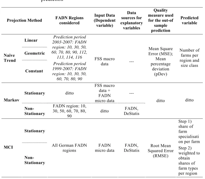
The regional coverage considered for the out-of-sample experiment differs between the projection methods (XTable 1X). The linear and geometric projections and the projection based on the stationary TP, which is estimated from FADN data, are performed for all FADN regions in Germany. Some FADN regions are excluded because of an insufficient number of observations (Hamburg (20), Bremen (40), Saarland (100) and Saxony-Anhalt (115)). The non-stationary projection and the stationary projection for the prediction period 1999-2007, however, are restricted to the West German FADN regions (excluding 20, 40, and 100), for which a time series from 1989 to 2008 is available.

(21)

Table 1: Characteristics of the different methodologies used in the out-of sample prediction

Projection Method FADN Regions _considered (Dependent Input Data

variable) Data sources for explanatory variables Quality measure used for the out-of

sample prediction Predicted variable Linear Geometric Naive Trend Constant Prediction period 2003-2007: FADN region: 10, 30, 50, 60, 70, 80, 90, 112, 113, 114, 116 Prediction period 1999-2007: FADN region: 10, 30, 50, 60, 70, 80, 90 FSS macro data --- Mean Square Error (MSE); Mean percentage deviation (pDev) Number of farms per region and size class Stationary ditto FSS macro data + FADN micro data --- Markov Non-Stationary FADN region: 10, 30, 50, 60, 70, 80, 90 ditto FADN, DeStatis ditto ditto Stationary MCI Non-Stationary

All German FADN

regions micro data FADN DeStatis FADN, Squared Error Root Mean (RMSE) Step 1) share of farm specialisati on per farm Step 2) weighted to obtain shares of farm types per region

In the Markov approach, we evaluate the performance of the out-of-sample prediction based on the calculation of mean square error (MSE) and mean percentage deviation (pDev) for each prediction method in each region. The MSE is calculated for each prediction method and region as the mean over the square difference between the predicted farm numbers and the observed farm numbers in each classF

1

F. Similarly, the mean percentage deviation is calculated as the mean over all farm types and classes of the percentage deviation of the predicted farm number from the true value derived from FSS. The latter measure is not defined in cases in which the true number of farms in a class is equal to zero; in this situation, the observation is excluded from the calculation of the mean percentage deviation.

(22)

The linear prediction is performed for each region, farm type and size class by estimating

1

γ and γ₂ of the linear function n_t =γ₁+γ₂t, where n_t is the number of farms in time t .

Using the estimates γˆ₁ and γˆ₂, farm numbers for t+1 are then predicted by

( )

1 ˆ1 ˆ2

ˆt 1

n+ =γ +γ t+ and for the following years accordingly. Macro data derived from FADN and the corresponding macro data grid available from EuroStat are used for the estimation. As in the Markov prediction, two time periods, one from 1989 to 1999 and one from 1989 to 2003, are considered in the estimation to predict farm numbers in 2007. The geometric growth rate is derived by estimating ln_{( )}nt = λ₁ +λ₂t. Farm numbers in t+1

are predicted using the estimated parameters _λˆ₁_and

2 ˆ λ to calculate (ˆ1 ˆ2( )1) 1 ˆ t t n+ =eλ λ+ + . The

data source and time periods are the same as those used for the linear prediction. An advantage of the geometric prediction is that in the linear case, the predicted farm number can become negative. However, problems arise in the geometric prediction in cases in which no farms are observed in a particular time period. In these cases, the dependent variable is not defined, and we omit the observation from the estimation.

We conduct out-of-sample predictions for the MCI approach analogously to the Markov approach for two different time periods. In the first case, we predict the change in the types of farming between 2003 and 2007 based on estimations derived from data recorded between 1989 and 2003. For the second out-of-sample prediction, only data from 1989 to 1999 are used to predict the farm structure in 2007. In contrast to the Markov approach, the MCI approach is purely based on the observed transitions at the farm level. Therefore, FADN regions with fewer records can remain in the sample. Only when the fit of the predictions is evaluated is it sensible to merge the data of smaller groups with similar larger groups to prevent deviations caused by small samples sizes that may affect the overall result.

As the MCI approach is based purely on the transitions observed in the FADN sample, it cannot depict changes in farm numbers, as exits from the sector are not recorded in FADN. Therefore, the evaluation of the out-of-sample prediction is based on the match of the predicted and observed farming structure, i.e., the share that the different types of farming have in the population. The root mean square error is chosen as an indicator and is calculated as follows:

(1):

where t is the type of farming, wr is the number of farms in region r, and se and so are the

estimated and observed share, respectively. XTable 1X provides a summary of the characteristics of all prediction methods with respect to the regional coverage that the data sources and the employed fit measure.

(23)

22B

1.2 Data

45B

1.2.1 Main

data

sources

Several aspects of the FSS and FADN databases differ (XTable 2X), which has implications for the analysis of structural change. First, FADN is not capable of depicting farm exits because it is a sample of the total population. Second, no inferences regarding the development of small farms can be made from FADN as small farms are not sampled. FADN is better suited to identify the influence of factors varying over time (e.g., market conditions) because of the high temporal resolution and the long time series. The high spatial resolution of FSS permits the formation of more reliable conclusions regarding factors varying over space (e.g., production conditions, availability of off farm income) and is less prone to problems regarding aggregation errors. An important practical difference regarding the development of methodologies to analyse structural change is that, within this study, the authors have access to FADN micro-data but not direct access to FSS micro-data. Therefore, to reduce the time demands associated with the implementation and debugging of the analytical programs, all analyses are first applied and tested using the FADN dataset. In particular, full access to FSS data would permit the development of incremental models capable of isolating the effect of changing SGM or SO.

Table 2: Differences between the FSS and FADN databases in Germany

FSS FADN

Type of data Full population Representative rotating sample of commercial farms; extrapolation to the population based on

farm-specific weighting factors Cut off limit > 2 ha or > 8 LU SGM: 1989-1998 (> 8 ESU) / 1999-2008 (> 16

ESU) Sampling

frequency 3-4 years interval Annually

Time series 1999, 2003, 2007 1989-2008

Spatial resolution LAU 2 (Local Administrative

Unit)

Farms identified at NUTS 3 level but sampling scheme based on NUTS 1 level

Information Structural Structural and financial

The German FADN sample provides a unique opportunity to use this approach because the farms remain in the sample for a long duration (XTable 3X). More than 12,000 farms remained in the sample for at least 4 years.

(24)

Table 3: Length of time that farms remained in the German FADN sample (1989-2008)

Years in the sample N° of farms

1 4334 2 2628 3 2642 4 1717 5 1391 6 1549 7 1133 8 1020 9 974 10 1366 > 10 3024

To retrieve the CAPRI classification of farm types, we use 8 data dimensions (XTable 4X). This classification fulfils the criteria of Equation X(28)X in Annex 3, in which the partial standard Gross Margin should equal unity. With the exemption of grazing livestock and permanent crops, the name of the dimension corresponds to the name of the specialised FADN types of farming on the 2-digit level. Extra dimensions are needed for grazing livestock. T4D corresponds to dairy cattle, whereas T4X sums the SGM of all male bovine, suckler cow, non-bovine and forage cropping activities. T4X is also needed to calculate the main specialisation (P1,…, P5). All decision variables for constructing the 2-digit FADN classification can be calculated with the proposed dimensions: e.g., for type of farming 71 (P1 = T13 + T14; P2 = T20; P3 = T30; P4 = T41 + T4D + T4X; P5 = T50).

Table 4: Classification of the FADN variables describing the farm structure to retrieve the 2-digit farm-classification and the CAPRI farm classification for Germany

Dimensions FADN variables considered to calculate the share of the total

SGM to define the step lengthF

2 F T13 D/1-D/9; D/22; D/26-D/30 T14 D/10; D/11; D/14a; D/19; D/20; D/23-D/25; D/31- D/35 T20 D/14b; D/15-D/17; I/2 T30 G/1 - G/7 T41 J/2; J/4; J/6 T4D J/7 T4X J/1; J/9; J/10; J/3; J/5; J/8; (D/12; D/18, F/1; F/2) T50 J/11-J18

The acronyms of the FADN variables are explained in Annex 1.

2

(25)

46B

1.2.2 Applied

typology

for the estimation

Data constraints and computational consideration of the Bayesian estimation approach need to be addressed to determine the degree of detail of specialisation and size classes for which farm numbers are projected, which limits the maximum number of classes. To maintain a sufficient degree of detail while keeping the number of classes manageable, farms belonging to classes characterised by very specialised production programs, such as

Specialist Horticulture, Specialist Vineyards, Specialist Fruit And Citrus Fruit, Specialist

Olives or Various Permanent Crops Combined, are excluded from the analysis.

Additionally, farm types with only a small number of farms in the sample are combined with other farm types that have relatively similar production programs. Finally, five different farm types, as defined in XTable 5X, are considered in the analysis. As a second dimension, in addition to the five different farm types, three size classes, defined as (I) 16-<40 ESU, (II) 40-<100 ESU and (III) >100 ESU, are considered. The restriction to three size classes and the specific definition of size classes are given by the FADN clustering scheme employed for Germany over the period 1989 to 2007.

Table 5: Definition of farm types considered for prediction

ID Name TF14 Description TF14

Code

1 COP crops Specialist Cereals, Oilseed And Protein Crops; Specialist Granivores TF13; TF5 2 Other crops Specialist Other Field Crops; Mixed crops TF14, TF6

(3 Horticulture Horticulture, Permanent Crops TF2;

TF3)

4 Milk Specialist Milk TF41

5 Other livestock Specialist Sheep and Goats; Specialist Cattle TF42, TF43, TF44

6 Mix Mixed Livestock; Mixed Crops and Livestock TF7,

TF8 Horticulture (ID 3) is only considered in the MCI approach.

47B

1.2.3 Treatment of the SGM

As solid information on structural change, i.e., the modification of the farm’s physical layout (e.g., machines, building and labour), is lacking in FSS and FADN statistical data, we use the agricultural enterprises crop and livestock shares based on the Standard Gross Margin (SGM) as a proxy of structural change. The SGM of a crop or livestock item is defined as the value of output from one hectare or from one animal less the cost of variable inputs required to produce that output. The SGM is used to define the Community Typology for agricultural holdings according to the Commission Decision 85/377/ECC amended by the Commission Decisions 96/376/EC; 96/373/EC; 1999/725/EC and

(26)

2003/369/EC. In Germany, the SGM is calculated for each NUTS 2 region and is updated annually. In the FADN database, to determine a farm’s farm type, the activities are weighted with a three-year average SGM. This procedure particularly dampens the impact of short-term price fluctuations. However, this average SGM is not a dynamic average but is kept constant for two or three years.

A pivotal issue in determining structural change over a longer time period is whether to use a time-variable or time-invariant (constant) SGM. A change to a time-invariant SGM could result in a different attribution (size and type of farming) for a given farm in both the FSS and FADN databases. Consequently, the FADN weighting factor must be adapted. Because time constraints, EuroStat was not capable of recalculating the grid based on constant SGMs within the time frame of this study.

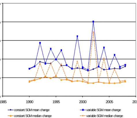
Figure 1: Comparison of the average (mean and median) annual changes in farm size (measured in € SGM) of German farms over time if the farms’ activities are weighted with a constant or variable SGM.

0% 5% 10% 15% 20% 25% 1985 1990 1995 2000 2005 2010 A n n u a l c h a n g e in f a rm s iz e ( in € S G M ) (i n % )

constant SGM mean change variable SGM mean change constant SGM median change variable SGM median change

Source: Own calculation based on the German FADN-farms during the period 1995-2007. Only farms that remained in the sample for at least two consecutive years are included.

However, the use of a variable SGM leads to severe problems in the estimation process and to counterintuitive results. First, the use of variable SGMs introduces additional dynamics regarding structural change that are not mirrored by a change in physical assets. When the SGM was updated, the recorded changes were 30% to 300% larger than those in years without an update. The updating influences the observed dynamics with regard to the changes in farm size (XFigure 1X) and also the specialisation (XFigure 2X). In years without an update of the SGM, the dynamic is independent of the year selected to weight the

(27)

farm’s activities. In the short run (interannual), most farms only marginally alter their structure in terms of both size and specialisation (see Annex 3, XFigure 22X-XFigure 25X). The distributions are right-skewed because the medians of the distributions are markedly lower than the means.

Figure 2: Comparison of the average (mean and median) annual change in the farm specialisationa_{of German farms over time if the farms’ activities}

are weighted with a constant or variable SGM.

0,00 0,02 0,04 0,06 0,08 0,10 1985 1990 1995 2000 2005 2010 St e p le n g th

constant SGM mean change variable SGM mean change

constant SGM median change variable SGM median change

Source: Own calculation based on the German FADN-farms in the period 1995-2007. Only farms that remained in the sample for at least two consecutive years are included.

a) measured by the step length using Manhattan Block metrics (for the calculation see Annex 3).

Second, even if three-year averages of the SGM are used, the SGM varies quite significantly over time. XFigure 3X depicts the development of the SGM per dairy cow over time for one German region. The price spike in 2000, which affected the SGM for 2002 and 2003, can clearly be observed. Only this price fluctuation would lead to an increase in the economic farm size of a pure dairy farm by more than 30% from 2001 to 2002 and a decrease by 15% from 2003 to 2004F

3

F. Consequently, an approach that determines structural change on the basis of a variable SGM would largely depict the changes in input and output prices but hardly any structural adjustments of the farms. Therefore, the calculations are based on the German NUTS 2 SGM in 2002. The weighting factors in the FADN sample were kept as stated for the MCI approach. In the Markov approach, in which valid weighting factors are required to derive the macro data, we use only fixed SGM for the time period of from 1999-2007, for which it is possible to recalculate farm weights based on the available FSS micro data. For years before 1999, it is not possible to

3

(28)

recalculate weights based on a fixed SGM because of the lack of FSS micro data. Consequently, variable SGMs are considered in the period of 1989 to 1999, whereas in the period of 1999 to 2007, the SGMs in 2002 are considered to calculate the economic size, farm type and weighting factor for each observation.

Figure 3: Development of the FADN-SGM per dairy cow in Upper Bavaria

(DE21) between 1986 and 2004.

0 250 500 750 1,000 1,250 1,500 1985 1990 1995 2000 2005 € p e r h e a d Source: EuroStat.

The presented methodology is independent of the method used to weight the activities (variable or constant SGM or Standard Output (SO)). Nevertheless, a change from, e.g., variable to constant SGM will have implications for the obtained results. After the accounting year 2010, the typology for agricultural holdings will be based on the SO (Commission Regulation 1242/2008/EC) rather than the SGM. The classification in both databases (FSS and FADN) is based on the SGM. This classification cannot be easily transferred to a SO-based classification as SO values are currently only available for 2004 and a change of the economic weight of the activities (from SGM to SO) would require the recalculation of the weighting factors in the FADN database. Therefore, we use the SGM approach in this study.

The farms are attributed to a type of farming based on the principles laid down in Commission Decision (2003/369/EC). As the data set with the lowest resolution determines the overall achievable data resolution, we have to omit the information for size classes 5 and 6 for the years prior to 1999, and we will interpret the output for the merged classes (9 and 10) because these classes were merged prior to 2004 (FADN, 2010).

(29)

48B

1.2.4 Explanatory

variables

X

Table 6X lists the explanatory variables that were identified in previous studies as determinants of structural change. The explanatory variables used in the non-stationary estimation of TP and the continuous approach are derived from the FADN dataset and from the public German database DeStatis. The geographical and time period availability are specified. The identified variables are broadly distinguishable by time and regional varying variables. Not all of the variables described in Table 5 were considered in the empirical applications because of limited data availability or high multicollinearity between explanatory variables. The final set of variables considered in the estimations is described in XTable 8X and XTable 9X.

(30)

Table 6: List of potential variables to be considered in an ex-post analysis and the likely data sources on the EU level

Group deter-minant

Indicator Proxy _sourceData

Variab le definiti on (con-structi on)

Unit graphical

Geo-resolutione Years Spatial coverage Technology FADNa =Table _K_col umn_q q / Table_ K_colu mn_A A tons / ha or tons per head

single farm,

FADN-region

1989-2008 EU

DeStatis _{tons per head}tons / ha or NUTS 3 1974-2010 Germany Yields

EUROST

ATb agr_r_c_rops 100 kg/ha NUTS 2 1977-2010 EU

Farm structure

Initial farm

size FADN =A27

Econ.size in EUR single farm, FADN-region 1989-2008 EU Initial farm

specialisation FADN =A30 4-digit Calculated by DG AGRI (c.f. Typology Regulation) single farm, FADN-region 1989-2008 EU Farm size

heterogeneity FADN Gini-Index; Shannon-Index FADN-region 1989-2008 EU Stocking densities FADN =SE08 0/SE02 5 LU per ha single farm, FADN-region 1989-2008 EU Share of

mixed farms FADN =Sum( SYS02 *(A30> =6000) )/Sum( SYS02 ) % FADN-_region 1989-2008 EU Market conditions FADN =(SA+ CV+F U+FC-BV)/Q Q

EUR per ton

single farm, FADN-region 1989-2008 EU Output prices

DeStatis Index Index NUTS 0 _(MS) 1989-2008 Germany Input prices DeStatis Index Index NUTS 0 _(MS) 1989-2008 Germany

Prices EUROST_AT Agr-r-_{aacts_} EUR NUTS 2 1974-2010 EU Land rent FADN

=SE37 5/SE02 5 EUR / ha single farm, FADN-region 1989-2008 EU Land rent DeStatis EUR / ha NUTS 2 1989-2008 Germany

(31)

Geo-resolutione Years Spatial coverage CAP 1st pillar CAP payments FADN Table M EUR single farm, FADN-region 1989-2008 EU

FADN Table J EUR

single farm, FADN-region 1989-2008 EU 2nd pillar

CAP payments CATS _(Clearanc e of Account database) EUR NUTS 3 2000-2005 EU 2nd pillar CAP payments Program mes Guidance , Guarante e, SAPAR D, Objective 1, IFDR, LEADER , EU27 (Agrex, Agriview ) EUR NUTS 1 2000-2007 EU FADN =SE37 5/SE02 5 EUR / ha single farm, FADN-region 1989-2008 EU Land rent

DeStatis EUR / ha NUTS 2 1989-2008 Germany

Natural resources FADN =(K147 AA+K 150AA +K151 AA)/S E025 % single farm, FADN-region 1989-2008 EU Share of grassland CORINE % LAU 2 _{2000, 2010}1990, EU

Slope USGSTO_{PO_30}d % 1 ha² 2000 EU

LFA FADN =A39 1,2,3

single farm, FADN-region 1989-2008 EU Climate Climate Data CRU-TS 1.2 Temperature 16 km² 1901-2000 EU

Natura 2K % EEA % scale 1:100 ₀₀₀ 2010 EU

Irrigated area CORINE % LAU 2 _{2000, 2010}1990, EU

(32)

Geo-resolutione Years Spatial coverage demographical factors EUROST AT Table:d emo_r_ poar NUTS 2 1990-2010 EU Populat ion density _DeStatis Inhabitants per km² LAU2 1974-2010 Germany EUROST AT Table:d emo_r_ poar NUTS 2 1990-2010 EU Popula-tion

growth _DeStatis % _{LAU2 1974-2010}_Germany Market distance Comm uting time to larger cities

BBSRc _Min _LAU_{2 2003}_Germany

Unemp loymen t rate EUROST AT Table: tgs000 07 % NUTS 2 1999-2007 EU Off-farm employment Relatio n Off-farm to farm income

FSS % farm, LAU single 2

1999,2003,

2007 Germany

Age FADN =C01Y_R Year

single farm,

FADN-region

1989-2008 EU a) The variable definition/construction refers to the FADN data warehouse variables.

b) The variable definition/construction is derived from the EuroStat-Agriculture database http://epp.eurostat.ec.europa.eu/portal/page/portal/agriculture/data/database.

c) The Federal Institute for Research on Building, Urban Affairs and Spatial Development (Commuting times) d) Earth Resources Observation and Science (Global 30-Arc Seconds elevation data)

e) The columns present the resolution at which representative results can be obtained.

In the following section, we will investigate the characteristics of some explanatory variables that we consider crucial for a more detailed estimation of structural change.

64B

1.2.4.1 Technology

Technological development over time can be approximated by variables that measure yield or by a trend variable. One obstacle in the definition of a yield variable is that it must measure the average yield variation over time for the entire farm type. This is straightforward for farm types such as the Milk class but problematic for more aggregated

classes such as the Mix class (ID 4 and 6, respectively, as reflected in Table 4). Two

possibilities are identified for a potential definition of a yield variable. One possibility is to define yield in terms of monetary output rather than physical quantities, which makes aggregation over different production activities feasible. The required data are available from the FADN ‘standard results’ for each of the different farm types (such as SE135

(33)

livestock output or SE131 Total output). The drawback of this approach, however, is that

that a substantial part of the fluctuation can be attributed to price fluctuation, which adds substantial noise to a variable intended to measure technological development over time. Another possibility would be to consider the yield for selected production activities as representative of the productivity of the entire farm type class. For COP crops and Other

crops, the yield of wheat (SE110) or the yield of maize (SE115) could be assumed to be

representative of the productivity in that year. For farm type Milk and Other Livestock,

milk yield (SE125) could be used. For the Mix farm type, one of the measures or a

combination of both could be selected. XFigure 4X shows the development of the average wheat, maize and milk yields. With the exception of a spike in the maize yield in 2007, which was likely caused by an unrealistically high outlier in that particular year, the average yield of each product closely follows a linear trend with little variation between years. This rather low variation is particularly problematic because the error of assuming that one particular crop represents the technological development in an entire farm type is supposedly rather large. Stated differently, the noise in the approximation appears to be substantial relative to the actual variation. Based on this discussion, we decided to consider a simple trend variable (defined as 1,2,..,T) that may be more appropriate to

capture technical improvements. The interpretation of this variable is also more intuitive because a yield variable that follows a linear trend would capture all other linear effects that evolve over time.

Figure 4: Development of the average yield of wheat (dt/ha; SE110), maize

(dt/ha; SE115) and milk equivalents (kg) per cow (SE115) (averaged over all Germany FADN regions)

Source: Own calculation from the FADN database.

(34)

65B

1.2.4.2 Prices,

subsidies and land rent

Output and input prices are derived from DeStatis for the time period 1988 to 2008. The database provides different price indices for different categories, which can be used for the different farm types. An index for crops (LANDWIRTPROD05) is used for COP crops

and Other crops, an index for milk (MILCH01) is used for Milk, and an index for

livestock products (TIERART001B) is used for Other livestock. For the Mix farm type, an

index for all agricultural products (LANDWIRTPROD01) is considered. All price indices

are considered in the logarithm. A price index for agricultural input prices

(BETRIEBMILAND01) is available for input prices. However, input prices are highly

correlated with a trend variable (as defined above) (which can also be observed in XFigure 5X) such that input prices must be excluded from the analysis to avoid multicollinearity.

Figure 5: Output and input price indices for different farm products

80 90 100 110 120 130 140 Prices indices for...

all ag. products crops livestock milk inputs

Source: Destatis 2011.

First and second pillar payments can be derived from the standard results in FADN for the different farm types (see XFigure 6X). Three problems, however, limit the use of first and second pillar payments as explanatory variables. First, subsidies have only been reported since 1993, which would effectively reduce the time series by 5 years if a lag of one year is considered; this would result in a time series from 1995 to 1999, or 1995 to 2003, which is problematic from a computational point of view. A second problem is the break in the policy regime in 2003/2004, during which coupled payments were phased out and decoupled payments were introduced. Because the policy change occurred after the time period used for the estimation, it is not possible to consider this break in the estimation or prediction.

(35)

Figure 6: Average subsidies (€/year) received per farm (West German FADN regions)

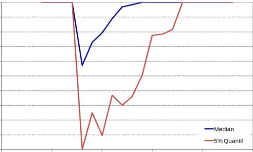
Third, the quality of the recorded data changed substantially during the recorded period. Especially in the mid-1990s, a non-negligible share of subsidies can be attributed to neither the first nor the second pillar. Only from 2003 onward does the sum of subsidies under the different subheadings equal the stated total.

Figure 7: Share of subsidies attributable to known sources for German FADN farms 0% 10% 20% 30% 40% 50% 60% 70% 80% 90% 100% 1985 1990 1995 2000 2005 2010 Sha re of subs id ie s at tr ibut abl e to know n s our ce s fo r Ge rm a n F ADN f a rm s Median 5% Quantil

Source: Own calculation from the FADN database (Relation of the aggregate of SE610, SE615, SE621, SE622, SE623, SE625, SE626, SE630 to SE605).

(36)

The average land rent in a region is calculated from FADN as the rent paid (SE375) divided by the rented Utilised Agricultural Area (UAA) (SE030). XFigure 8X depicts the development of the average land rent for the two selected regions, Lower Saxony and Bavaria, over time. In the estimation, the average land rent is considered on a log scale and lagged by one year.

Figure 8: Average land rent per ha (West German FADN regions)

66B

1.2.4.3 Socio-economic variables

The off-farm employment opportunities can be approximated by the unemployment rate (XFigure 9X). The unemployment rate (calculated for the civil dependent labour force) is available from Destatis for the German Laender for the time period 1991 to 2008 and from Statistisches Bundesamt (1993) for 1988 to 1991. Figure 9 clearly shows that the development of the unemployment rate is highly correlated among the FADN regions and the differences in the unemployment rate in 2008 can be largely attributed to a base effect (unemployment rate in 2008).

(37)

Figure 9: Unemployment rate of the civil dependent labour force

Source: Destatis 2011 and Statistisches Bundesamt (1993, p. 128).

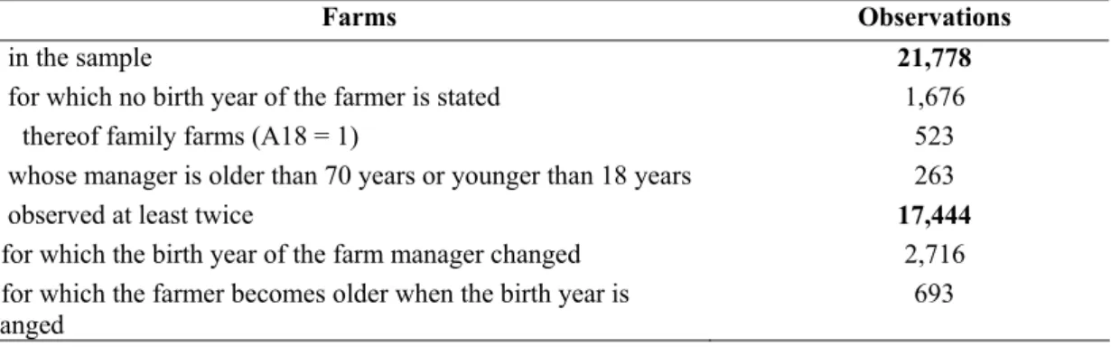
Frequently, a change in the farm structure coincides with the handover of the farm business. Therefore, a change in the farmer’s age could be a reasonable proxy for changes that are occurring in the farm structure or are going to occur in the near future, which makes a closer examination of the FADN-variable C01YR worthwhile (XTable 7X). For roughly 1,700 farms (7.7% of the total population), no birth year is stated. Most of these holdings are not family farms. Within the sample, more than 2,700 changes in the age of the farm manager are recorded. However, in nearly a quarter of these cases, the farm manager becomes older upon the transition. It seems unlikely (based on the theory and rationale) that the proportion of farms that is handed over from the younger to the older generation is this high, and therefore, we assume that this variable does not accurately reflect reality.

Table 7: Overview of some key figures regarding the age information in the German FADN sample (1989-2008)

Farms Observations

… in the sample 21,778

… for which no birth year of the farmer is stated 1,676

thereof family farms (A18 = 1) 523

… whose manager is older than 70 years or younger than 18 years 263

… observed at least twice 17,444

…for which the birth year of the farm manager changed 2,716 …for which the farmer becomes older when the birth year is

changed 693

(38)

67B

1.2.4.4 Natural

conditions

The distribution and development of farm types is dependent on the natural conditions (e.g., temperature, precipitation, slope). For instance, in Bavaria (FADN region 90), dairy farming retreated in the last decade from areas suitable for arable farming (DICK and

HETZ, 2011). XFigure 10X shows the differences in the average conditions faced by the different farm types in the German FADN regions for two selected variables (average summer temperature and average slope). Marked differences exist among the farm types for these two factors, even within one region, and these factors determine plant growth and available field labour days. For instance, in the Southern and Western FADN regions (see Annex 2), dairy farms tend to be located in cooler and hillier regions when compared with cereal farms. It is reasonable to assume that the relative efficiency of the different farm types differs with regard to their sensitivity to these environmental factors. This may,

ceteris paribus, imply that a dairy farm in an area with warmer and drier conditions is

much more likely to expand cash cropping than a farm facing a cooler and more humid climate.

Figure 10: Average summer temperature and slope for the different farm types in the German FADN regions

12 13 14 15 10 20 30 50 60 70 80 90 100 112 113 114 116 A v g . su mmer t e m p er a tu re ( in ° C ) Region (A1) FT_13_50 FT_14_60 FT_20_30 FT_41 FT_42_43_44 FT_70_80 0% 1% 2% 3% 4% 5% 6% 7% 10 20 30 50 60 70 80 90 100 112 113 114 116 A v g. slope of t h e ar ic ult rual ar ea ( in % ) Region (A1) FT_13_50 FT_14_60 FT_20_30 FT_41 FT_42_43_44 FT_70_80

(39)

Source: Own calculation based on the FADN database, BKG (2007) and DWD (2009).

49B

1.2.5 Implementation

of

the data in the final estimation approaches

All time-varying explanatory variables are considered with a lag of one year because we expect that adjustments will occur with some delay. This implies that the first year needs to be omitted from the estimation if explanatory variables are not available prior to the first year considered.

The variable sets vary between the two estimation approaches (Markov and MCI), as the MCI (because of the higher number of observational units) is better suited to the depiction of the influence of time-invariant factors (e.g., climateF

4

F, terrain, commuting time). As these factors can hardly be influenced by political decisions, their inclusion actually improves the trend prediction. The Markov approach focuses on the influence of time-variant variables and depicts time-intime-variant differences among regions using a regional dummy.

The selection (Markov and MCI approach) of the sets of explanatory variables is based on the Akaike Information Criterion (AIC). The AIC provides a trade-off between goodness of fit and the simplicity of the model. A general-to-specific selection process is adopted in which we start with the largest model, including all explanatory variables, and subsequently exclude variables as long as their exclusion results in a lower AIC. The specification with the lowest AIC is chosen as the final specification.

In all Markov models a constant and regional dummy variables are considered for all regions except one. The exclusion of the constant or a regional dummy variable is not considered in the model selection process, and thus the constant and all regional dummy variables are included in all models. In the MCI models, the constant and the lagged shares of the specialisation are excluded from the selection process.

Because of the described data problems regarding subsidies, the different public support regimes are depicted in the Markov approach by two different dummy variables. In particular, a dummy variable for the MacSharry reform (zero for t≤1992 and one afterwards) and a dummy variable for the Agenda 2000 (zero for t≤1999 and one afterwards) are considered. Despite these problems, the payments are implemented in the continuous approach as continuous variables.

4

(40)

X

Table 8X provides the final selection of all explanatory variables used in the Markov approach for the different farm types. The primary data source for the Markov out-of-sample prediction is the FADN database and the corresponding macro data grid available from EuroStat. Micro data can be derived directly from FADN because the farms, which are uniquely identified in the dataset, are observed over time. Macro data can be derived by considering the weights attached to each sample farm. These weighting factors are calculated based on the Farm Structure Survey (FSS), which is conducted every three or four years, and reflect the number of farms that a sample farm represents in the population. Using these weighting factors, it is therefore possible to recalculate the total number of farms in the population within classes of specialisation and size from the FADN sample. One obstacle is that, even though FADN data are available on a yearly basis, the weights are calculated based on the latest FSS information, which is only available every two to three years. This leads to breaks in the macro data such that farm numbers in the categories change only every two to three years. To address this factor, farm numbers are approximated between FSS years using a calculated geometric growth rateF

5

F (a linear approximation could have also been used, but a relative growth rate was assumed to be more appropriate).

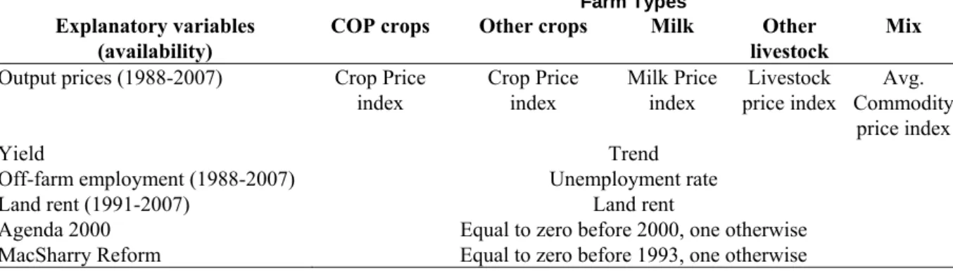
Table 8: Time-varying explanatory variables for the different farm types selected in the Markov approach

Farm Types

Explanatory variables (availability)

COP crops Other crops Milk Other

livestock

Mix

Output prices (1988-2007) Crop Price index Crop Price index Milk Price index Livestock price index Avg. Commodity price index Yield Trend Off-farm employment (1988-2007) Unemployment rate

Land rent (1991-2007) Land rent

Agenda 2000 Equal to zero before 2000, one otherwise MacSharry Reform Equal to zero before 1993, one otherwise

X

Table 9X lists the explanatory variables ultimately used in the MCI approach. In principle, the MCI approach uses the same data sources as the Markov approach. Some additional data sources are used to derive time-invariant information for the region. Whereas a price index is implemented in the Markov approach, relative price changes are used in the MCI models. As year-to-year changes in the structure of individual farms are fairly small and

5

The geometric growth rate is calculated by 1 0 1 0

t t

r = − n n , where nt is the number of farms in t.

Farm numbers are predicted between FSS years using

(

)

0 0 1

t t

t t

n =n +r − . For example, for the years between the FSS 1990 and 1993, the geometric growth rate is calculated by 1993 1990

1999 1990

r = − n n ,

(41)

largely random (XFigure 23X), we use a four-year period rather than a yearly interval in the MCI approach. An advantage of this interval is that the results can be directly compared with an analysis based mainly on FSS data.

Table 9: Variables used in the MCI approach

Estimation period Type of

variable Variable Comment 1999)

(1989-2003)

Price (1988-2008)

Soft wheat EuroStat: Agr-r-aacts X X

Durum wheat ditto X X Rape seed ditto X X

Flowers ditto X

Sugar beet ditto X X

Grass ditto X

Beef ditto X

Farm (1989-2008)

Farm size log of the farms SGM X Interest Relationship of paid

interest to SGM X X

Age Year X

Tenure € per ha X Share of rented land % X Stocking density LU per ha X

Share of grassland on UAA

% _X

Farm diversification Shannon index based on 8 and 14 different specialisations

X X Total subsidies Relationship of total

subsidies to SGM X X Subsidies 1st_pillar _{Relationship of subsidies}

to SGM X

Subsidies 2nd_pillar _{Relationship of subsidies}

to SGM X Subsidies agri-environment Relationship of subsidies to SGM X Region Summer temperature (Avg. of 1961-1990) DWD (2009) X Winter temperature (Avg. of 1961-1990) ditto X X Annual precipitation (Avg. of 1961-1990) ditto X Winter precipitation (Avg. of 1961-1990) ditto _{X X} Water balance (Avg. of 1961-1990) ditto _X Commuting time (2003) BBSR X X Avg. Population density EuroStat: X X

(42)

(1997-2008) demo_r_d3dens Change in population

density (1997-2008)

ditto

X Avg. Employment rate

(1999-2008) EuroStat: tgs00007 _X Change in employment rate (1999-2008) ditto _X Share of grassland BKG (2007) X Altitude BKG (2007) X Slope BKG (2007) X Natura 2K % EEA