A Dissertation by YIXIN CAO
Submitted to the Office of Graduate Studies of Texas A&M University
in partial fulfillment of the requirements for the degree of DOCTOR OF PHILOSOPHY
May 2012
A Dissertation by YIXIN CAO
Submitted to the Office of Graduate Studies of Texas A&M University
in partial fulfillment of the requirements for the degree of DOCTOR OF PHILOSOPHY
Approved by:
Chair of Committee, Jianer Chen Committee Members, Sergiy Butenko
Donald K. Friesen Tiffani Williams Head of Department, Duncan M. Walker
May 2012
ABSTRACT
Clustering and Inconsistent Information: A Kernelization Approach. (May 2012) Yixin Cao, B.E., Harbin Engineering University; M.S., Beijing University of
Aeronautics and Astronautics
Chair of Advisory Committee: Dr. Jianer Chen
Clustering is the unsupervised classification of patterns into groups, which is easy provided the data of patterns are consistent. However, real data are almost always tempered with inconsistencies, which make it a hard problem, and actually, the most widely studied formulations, correlation clustering and hierarchical clus-tering, are both NP-hard. In the graph representation of data, inconsistencies also frequently present themselves as cycles, also called deadlocks, and to break cycles by removing vertices is the objective of the classical feedback vertex set (FVS) problem. This dissertation studies the three problems, correlation clustering, hierarchical clustering, and disjoint-FVS (a variation of FVS), from a kernelization approach. A kernelization algorithm in polynomial time reduces a problem instance provably to speed up the further processing with other approaches. For each of the problems studied, an efficient kernelization algorithm of linear or sub-quadratic running time is presented. All the kernels obtained in this dissertation have linear size with very small constants. Better parameterized algorithms are also designed based on the kernels for the last two problems.
Finally, some concluding remarks on possible directions for future research are briefly mentioned.
ACKNOWLEDGMENTS
Now stepping on the last stair after such a long journey, it is a perfect time to look back. Before myself is a tortuous road, and only with many helps from many people I can finally finish it. I bad been almost lost, squandering several years without knowing I was born to do, until I came back to campus as a graduate student. In the past four years I really enjoyed the tranquil life in the small town in beautiful middle Texas, and the happiness it bestows on me is only second to my academical life. Undoubtedly I owe many thanks to a lot of people, especially for those who have helped to bring me back to track.
It is hard to express my sincere gratitude to my adviser, Dr. Jianer Chen. He introduced me into this area, and more importantly, reignited my passion in algorithmic design and mathematics. His individualized advising style makes him an ideal adviser. For me this implies great freedom. The freedom to choose what to study and where to go is so essential for me that I cannot imagine the otherwise. The free and equal communication atmosphere between us is another benefit.
It is the same hard to express the profound influence of my brother, also a Ph.D. in computer science, on me during this journey. His encouragement was critical at the beginning, when I had not made the decision, and his valuable suggestions and advice were important in each stage.
I would also like to thank my committee members, Dr. Sergiy Butenko, Dr. Donald K. Friesen, and Dr. Tiffani Williams, for their precious time and help.
Nearly half of my time was spent in office, with the guys (literally, guys) in the research group led by my adviser. We together created a great environment for research. It was a great pleasure working with them: Dr. Yang liu, Jia-Hao Fan, Qilong Feng, and Cheng Cao. Although I joined this group only half-year before his
graduation, Yang and I had a wonderful collaboration. Qilong and I shared office in more than one year, during that time we had many valuable discussions. I also want to thank my labmats in Parasol in my first year: Dr. Jacob Smith and Xiaolong Tang, who helped a lot at the early stage of my Ph.D. study.
The Department of Computer Science at Texas A&M University provided fi-nancial support for my whole Ph.D. study. During these years, I have been working as Teaching Assitant, Research Assitant, and Unix Administrator, and thus worked together with a lot of faculty and staff. Besides relieving my finiancial pressure, the work experience itself helped me a lot.
TABLE OF CONTENTS
Page
ABSTRACT . . . iii
DEDICATION . . . iv
ACKNOWLEDGMENTS . . . v
TABLE OF CONTENTS . . . vii
LIST OF TABLES . . . ix LIST OF FIGURES . . . x 1. INTRODUCTION . . . 1 1.1 Parameterized Computation . . . 2 1.2 Kernelization . . . 5 1.3 Clustering . . . 7
1.4 Feedback Set Problems . . . 10
1.5 A Big Map . . . 11
1.6 Outline of This Dissertation . . . 13
2. LITERATURE REVIEW AND DEFINITIONS . . . 17
2.1 General References and Notations . . . 17
2.2 Parameterized (Exact) Computation . . . 18
2.3 Kernelization Algorithms . . . 23
2.4 Clustering . . . 31
2.5 Feedback Sets . . . 36
3. CORRELATION CLUSTERING . . . 40
3.1 Cutting Lemmas . . . 42
3.2 The Reduction Steps . . . 46
3.3 The Kernelization Algorithm . . . 54
3.4 On Unweighted and Real-Weighted Versions . . . 57
3.5 Discussion . . . 62
4. HIERARCHICAL CLUSTERING . . . 64
Page
4.2 The Kernelization Algorithm . . . 71
4.3 The Parameterized Algorithm . . . 80
4.4 Discussion . . . 85
5. FEEDBACK VERTEX SET . . . 86
5.1 Disjoint-FVS and Its Kernel . . . 87
5.2 A Polynomial-Time Solvable Case for Disjoint-FVS . . . 96
5.3 An Improved Algorithm for Disjoint-FVS . . . 105
5.4 Concluding Result: An Improved Algorithm for FVS . . . 110
6. SUMMARY AND FUTURE RESEARCH . . . 113
6.1 Dissertation Summary . . . 113
6.2 Parameterized Complexity of Multiway Cut . . . 115
6.3 Approximation of Correlation Clustering . . . 118
6.4 Other Possible Directions . . . 119
REFERENCES . . . 122
LIST OF TABLES
TABLE Page
1.1 The comparison ofcn for c=2, 1.414, 1.260, 1.1 . . . 3
1.2 Variations of feedback set problems. . . 10
2.1 Previous results for the correlation clustering andM-hierarchical cluster-ing problems . . . 36
2.2 The history of deterministic parameterized algorithms for FVS . . . 38
5.1 Moving the vertex v fromV1 toV2 . . . 92
LIST OF FIGURES
FIGURE Page
1.1 An example of hierarchical clustering . . . 9
1.2 The major problems under parameterized study . . . 12
4.1 An instance of hierarchical clustering that cannot be solved greedily . . . 81
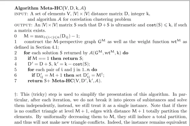
4.2 A meta-algorithm for hierarchical clustering . . . 83
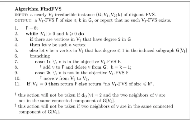
5.1 A simple branch-and-bound algorithm for disjoint-FVS . . . 90
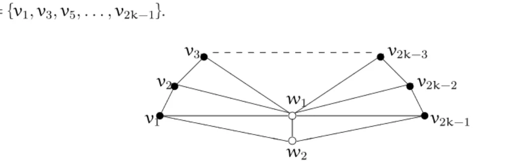
5.2 An example showing the tightness of Corollary 5.6 . . . 95
1. INTRODUCTION
In a time dubbed as “information age”, to handle information (data) is one of the most important tasks of human life, and can be roughly divided into two stages: “data collection” and “data analysis”. Given that in real life there are no perfect methods to collect data, the data we are going to analyze are always supposed to be tempered with errors, and then one immediate problem is, how to retrieve the valuable information from the raw data by removing errors and inconsistencies.
One rich field where data keep spraying in a speed of gigabytes per day is the computational biology and life science. Every species in nature is complex, and even the DNA of a single-celled microorganism is complicated enough to carry large quantities of data, not to mention complex lifes or even human being. Thanks to remarkable efforts of generations of biologists, more and more raw genome sequences have been accumulated via experimental methods. From these collected data, with possible errors present, computational biologists try to, among others, classify the species , e.g. to identify similar genome sequences. The classification task has many different formulations that are, from the computational aspect, collectively called clustering problems. They turn out to be universal and can be found in many disciplines.
Not equipped with answer checkers, a challenge presents itself at the beginning and has to be answered before anything else is, what is a solution? Various models have been formulated on coping with inconsistencies, under different assumptions. Among them the most widely taken one should be that the erroneous data are very limited compared to the whole data set, so solutions with the minimum amount of inconsistencies are looked after. In other words, it is assumed that the solutions
with the fewest errors are the most plausible. Computational problems formulated under this stipulation are all, unfortunately, NP-complete, and therefore unlikely have efficient algorithms runnable in polynomial time. In this case, people turn to other options. One is to sacrifice the optimality, trying to find a “reasonably good” solution in polynomial time. According to whether quality of the solution is guaran-teed or not, algorithms in this category can be further labeled with approximation and heuristic. The other option is to allow “moderately exponential runtime”, while the solution must be optimal. As a complement to both options, before losing the optimality and starting the exponential time process, we can pre-process the problem first, by significantly reducing it, and then relay it to other approaches. This step is known as kernelization, and should be conducted efficiently, usually in polynomial time. The outcome of kernelization, the reduced problem, is called a kernel.
This dissertation, as indicated in its title, takes the kernelization approach. It starts from searching the limit that the kernelization step can reach on the problems under investigation, and then turns to the application of the obtained kernels in later approaches. The remainder of this section is a short introduction to the theoretical framework as well as the problems studied in this dissertation. All technical details will be deferred to later chapters, in the hope that this chapter can be kept as simple as possible.
1.1 Parameterized Computation
By definition, all NP-complete problems are equivalent in the sense of poly-nomial time solubility, while under some complexity hypotheses, their exponential solubility is disparate. Some problems, e.g. SAT, never witness an algorithm faster
than O(2n)1, — such one, if exists, will be a breakthrough [167] — while some have far better algorithms, e.g. subexponential or pseudo-polynomial. Under the widely accepted assumption P 6= NP, some exponential explosion is inevitable in the time complexity of any algorithm for an NP-hard problem. On this ground, people turned to algorithms withmoderatelyexponential runtime that, though still exponential, in-creases far slower than O(2n).
This is a road on which many people have set foot. One notable candidate for moderately exponential functions is cn (c < 1). Normally, for an exponential
function f(n) =cn, any small decrement of the basec will significantly decrease the
value when n is large. Nevertheless, even cis as small as 1.1, and n is not too large (say n = 1000), cn is still prohibitive. See Table 1.1 for a comparison (note that
1.414=21/2 and 1.260=21/3).
Table 1.1
The comparison ofcn forc=2, 1.414, 1.260, 1.1
n 10 20 30 40 50 100 1000
2n 1024 1048576 1.1·109 1.1·1012 1.1·1015 1.3·1030 1.1·10301 1.414n 32 1024 32768 1048576 3.4·107 1.1·1015 3.3·10150 1.260n 10.08 101.59 1024 10321 104032 1.1·1010 2.2·10100 1.1n 2.59 6.73 17.45 45.26 117.40 13780 2.5·1041
In spite of their hardness, problems have to be solved, and heuristic is the tag most frequently seen on the weapons used to fight such problems in practice. Those heuristic methods, used independently or in combination with others, take advantage of the special characteristics of the inputs from the real applications, and disregard
1Although there are no mathematical proofs, it is believed that NP-complete problems are solvable
most artificial worst cases. Among those benign characteristics, the following two are the most frequently observed:
• only solutions of a small size are meaningful, while a solution of a size exceeding a problem-specific threshold is useless, and always disregarded;
• special structures always exist in real applications, such as (when formulated graph-theoretically): the maximum degree of vertices in the graph is upper bounded by a constant independent of the number of vertices; the graph is very sparse (or dense); it is easily decomposable into connected components (there are small separators).
Employing these inspiring facts, numerous efficient algorithms have been developed. In other words, although the problems are hard in general, the hardness can be (par-tially) relieved when some structural conditions are satisfied. This property turned out to be very general and observed in many problems, on which systematized stud-ies have been conducted, resulting in a new area on algorithmic study, parameterized computation.
The main idea in the core of such algorithms is the same: to identify some parameter of small size (k) independent of the problem size (n) which catches the hardness of the problem at hand (solution sizes, structural measures, etc.), and then restrict the exponential explosion of time complexity only to this parameter. The outcome then is another type of super-polynomial functions (note we cannot do away with it totally assuming P 6= NP) of the form f(k)·nc, where f is a computable function2 dependent only on k and c is a constant independent of k. Since the parameter k is far smaller compared to the input size n, this time complexity is arguably better than any exponential function on n. More importantly, when k is
not large, such algorithms can be implemented and executed in modern computers, which makes this direction very promising.
Albeit rooted from the similar observations of de facto favor, parameterized computation, built on a rigorous theoretic framework, deviates from the heuristic ap-proach significantly. This well-defined theory classifies problems in a two-dimensional way (compared to the one-dimensional classification of traditional complexity the-ory), and suggests that only fixed-parameter tractable problems admit such algo-rithms. Twoinformal comparisons might reveal some intuitions of the demarcations: 1. most NP-complete problems admit O(2n)time algorithms, trivial or not; 2. if the
solution size is k, many problems can be solved in O(nk) time by enumerating all
subsets with size no more thank. The latter one,O(nk), is polynomial ifkis a fixed
constant, however, it is still not practical even if kis as small as 10. Informally and roughly, we can say O(f(k)·nc)<O(nk)<O(2n), where the symbol “<” should be interpreted as “better than”.
1.2 Kernelization
Facing a problem hard to be solved directly, people would usually try splitting and/or reducing it, and see what is going on. This technique, in its intuitive sense, is so natural that people can master it without any learning. As examples for its occurrences in algorithms:
• when solving the SAT problem, one comes to single-literal clauses first;
• when solving the independent set problem, one only needs to work on the connected components separately.
This list can be very long, and indeed, such steps exist in almost all non-trivial com-puter programs. Neverthelss, they seldom, if ever, appear in literature on theoretical algorithms (heuristic algorithms are exceptions). The awkward discrepancy can be explained by the rigorous nature of worst-case time complexity analyses in theoretical algorithms, and the fact that above steps were believed to be not applicable for worst cases. This situation changed within the framework of parameterized computation, where the irreducible worst cases normally come with big solution sizes, and thus not interest us. As a matter of fact, the study of kernelization algorithms, previously called “preprocessing and data reduction”, can be somehow viewed as a systematic study of such preprocessing steps, complemented by bounding techniques.
Kernelization algorithms, given an instancex and an integer k, in time polyno-mial to (x+k), produce an equivalent and reduced instancex0 and a smaller integer k0 such that the size of the x0 (|x0|) is bounded by a function of k0. Here by equiv-alent we mean the original instance x has a solution with size no more than k if and only if the reduced instance x0 has a solution with size no more than k0. The reduced instance is called the kernel because we assume it is the really hard part of this problem, and for any algorithmic attack running in polynomial time there must be some kernels not surrendering, unless the polynomial hierarchy collapses. Note that the kernel size |x0| is not necessarily bounded by a polynomial function of k0, and when it does, we call it a polynomial kernel.
It is trivial that a problem is in FPT if it has a kernel, because after the kernel is obtained, whatever algorithms you apply to it, the time is only related to k, and the total time isf(k)·nc. The other direction, albeit not so obvious, also holds true.
In other words, a problem is fixed parameter tractable if and only if it admits a kernel. This theorem connects these two concepts in principle, and then only the existence of polynomial kernels is of its own interest. This dissertation will only
be concerned with polynomial kernels, and unless explicitly specified otherwise, all kernels mentioned in this dissertation are polynomial ones.
In literature, a traditional algorithm is described in three parts: first the pro-cedure of the algorithm, second a proof of its correctness, and finally an analysis of its time complexity. A kernelization algorithm is a little special, in this sense that it involves one more part, the analysis of the kernel size. This is always the focus, and usually the only non-trivial part, of a kernelization algorithm. This feature is mainly due to its heuristic nature: the procedures of most kernelization algorithms can be explained with one or two sentences; their time complexity analyses are trivial; and the correctness of many works is straightforward (exceptions exist, some latest results do involve complicated arguments).
Historically, kernelization algorithms originated from the study of parameter-ized computation, and were seen in almost all such algorithms ever published. Later, their applicability was found outside of parameterized computation, and they began receiving interests out of parameterized computation community. This transforma-tion escalated after more parameter-independent results, and nowadays, it ripens to call the study of kernelization algorithms as an independent research area. Other than designing kernelization algorithms for concrete problems, this dissertation will also study the several aspects of the nascent theorization of kernelization.
1.3 Clustering
One of the most common tasks in data analyses is to classify a (usually large) set of elements based on their relevance (the data collected). This is calledclustering, and informally defined By Jain, Murty and Flynn [131] as “the unsupervised classi-fication of patterns into groups (clusters)”. Clustering has incarnations in so many
disciplines, including biology, archaeology, geology, geography, business management, and social sciences, and has been approached by statisticians, mathematicians, com-puter scientists as well as industrial engineers.
To construct such a classification is not hard, provided the given data are perfect, or consistent. The requirement of a data set to be consistent is simple: if element a is determined to be similar to elementb, andb is similar to elementc, then amust be also similar to c. Unfortunately, there are seldom, if any, data collection methods which can exclude possibilities of errors and inconsistencies. As a consequence, real data always come with errors and in the computational sense, to remove those noise (incorrect information) is equivalent to do the classification.
To exacerbate the situation, we do not have a answer checker, and thus can never know how far our answers are from the reality. Various models have been proposed to measure the solutions, of which the most popular one is “minimum number of modifications”, whose basic idea is that the ratio of errors is low in most cases. On one hand, we assume the data to be almostconsistent, and this is really the case for most modern experiments where instruments and methods have been improved so much. On the other hand, if some data contain too many errors, it does not make sense to use them at all, and we have to repeat the data collection.
Corresponding to make the data consistent with the least amount of modifica-tions, a graph-theoretical formulation of the problem is called correlation clustering that seeks a collection of edge insertions/deletions with the minimum number (or cost when it is weighted) that transforms a given graph into a disjoint union of clusters (cliques).
The correlation clustering model has a flat structure, which is simply a parti-tion where each object belongs to exactly one cluster. Thanks to its simplicity and theoretical beauty, this model has been widely used and intensively studied.
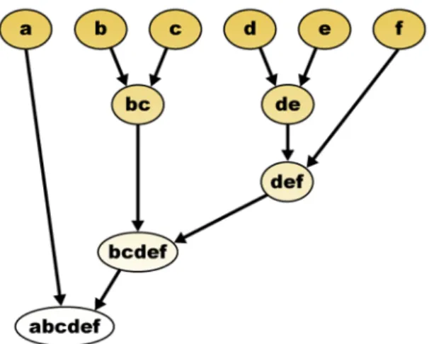
How-Fig. 1.1. An example of hierarchical clustering
ever, this simplicity comes with cost, and there are many applications whose rich structural information does not fit into a one-level classification. For an instance, to classify six animals: cat, tiger, dog, wolf, frog and toad, we can use three clusters, i.e. (cat, tiger), (dog, wolf) and (frog, toad). This classification is meaningful, but not sufficient, and it is easy to see that the first two classes are closer compared to the last one, which is impossible to be represented in a flat structure. In this case, a two-level structure should be more appropriate, i.e. (((cat,tiger),(dog, wolf)), (frog, toad)). When more species have to be considered, more levels might be needed, and the obtained result should be a structure similar to Figure 1.13.
Usually, the relevance between each pair of elements is measured by their dis-tance, and the smaller the more similar. Inspired by above discussion, we also con-sider the hierarchical structure, such that the data are arranged into a tree structure. All objects are the leaves at level 0, and each non-leaf vertices are at levels between 1 and M+1, such that the distance between two objects is the level of their first
common ancestor. By definition the root node is at levelM+1. Such a tree is called the M-hierachical clustering tree.
The M-hierachical clustering, very similar to correlation clustering, asks for the minimum number of total modifications to make the given data set into an M-hierachical clustering tree.
1.4 Feedback Set Problems
Feedback sets problems are a collection of problems, whose objective, as the name suggests, is to break all cycles in the given (di)graphs by removing vertices or edges/arcs. There are several incarnations based on the type of the input (di)graphs, and the specified operations. The graphs can be an undirected graph, a digraph, or a tournament, which is a special digraph4.
Table 1.2
Variations of feedback set problems.
vertices edges/arcs
Undirected FVS maximum spanning tree
Directed directed FVS FAS
Tournament FVS in tournaments FAS in tournaments
This gives six variations, enlisted in Table 1.2, of which five are NP-hard. The only exception is maximum spanning tree, which is equivalent to the famous min-imum spanning tree problem. Thanks to their theoretical importance and wide applications, FVS, DFVS, and FAST are all very popular research topics, where the other two, FAS and FVST, receive only marginal consideration. Particularly, FVS and FAST will be studied in this dissertation.
In operating systems, DFVS play a prominent role in the study of deadlock re-covery. In the wait-for graph of an operating system, each directed cycle corresponds to a deadlock situation. In order to resolve all deadlocks, some blocked processes have to be aborted. A minimum DFVS in this graph corresponds to a minimum number of processes that one needs to abort. They can also be found in database system, genome assembly, and VLSI chip design.
The feedback arc set in tournaments (FAST) is the FAS problem restricted to tournament. Thanks to increasing interest on data mining, search engine, as well as artificial intelligence, this problem has becomes a hot topic in theoretical computer science, and its identity of NP-completeness was finally settled recently.
Interestingly, the FAST problem is also closely related to correlation clustering problem. They are both. Some techniques are applicable to both, among which the most important ones are linear program and modular decomposition, and in particular, they can be formulated into exactly same linear program.
1.5 A Big Map
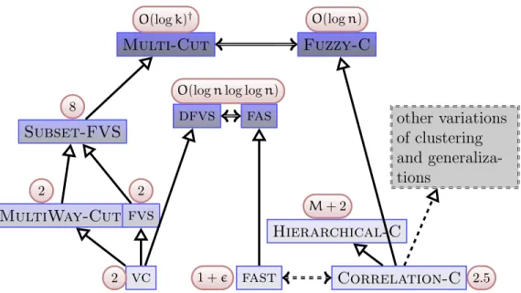
As usual, the best way to understand some topics is to put them into a big map, where the related topics and especially their relations present, even most of them are not of direct interest. To understand the problems studied here from algorithmic aspect, the big map comprising the major problems currently under parameterized study, is depicted in Figure 1.2. These problems are listed by increasing hardness (informally and intuitively) from bottom to up, and beside each problem its best approximation ratio is algo given. All of these problem have been shown to be in FPT, however, for most of them no polynomial kernel is known. The five problems listed here which have not been mentioned above are: 1. Vertex Cover (VC) asks for
vc fast Correlation-C MultiWay-Cut fvs dfvs fas Hierarchical-C other variations of clustering and generaliza-tions Subset-FVS Multi-Cut Fuzzy-C 2 1+ 2.5 2 2
O(lognlog logn)
M+2 8
O(logk)† O(logn)
A B means that problems Aand B are computationally equivalent. A B means that problem A is a special case of problemB.
A B means that problems A and Bbear striking resemblance, but are not equivalent.
A B and the dashed box mean that problem Band their relation are not clear yet.
2 is the best known approximation ratio of this problem.
†: k is the number of pairs of requirements.
Fig. 1.2. The major problems under parameterized study
a minimum set of vertices which are incident to all edges. 2. MultiWay-Cut asks for a minimum set of vertices (or edges, then also called MultiTerminal-Cut) whose
removal breaks all path between any pair of vertices from a given set of terminals. 3. Subset-FVS asks for a minimum set of vertices whose removal breaks all cycles through a given subset of vertices. 4. Multi-Cut asks for a minimum set of vertices (or edges) whose removal breaks all path between each pair of vertices as given. 5. Fuzzy-Clustering asks for a minimum number of edge addition/deletion to make a graph into disjoint union of cliques, where some pairs bear no cost.
1.6 Outline of This Dissertation
This dissertation starts from a comprehensive survey and literature review in Chapter 2, which also contains the formal definitions of the problems studied, as well as the general notations on graph theory, algorithms, and complexity theory. After that, the concrete results are presented in order.
Chapter 3 studies the correlation clustering problem, and develops the first ker-nelization algorithm for its weighted version, which in sub-quadratic time produces a 2k-vertex kernel. The algorithm (Section 3.2) is not the only contribution of this chapter, and is preceded by a series of cutting lemmas (Section 3.1), which is a re-sult of a thorough study of the structural specialties of this problem by relating it with graph edge-cuts. Following from a simple observation: a densely connected subgraph with very sparse connection to outside vertices should make a cluster, the reduction steps used to obtain the kernel are extremely simple. The only structure involved in the reduction is the closed neighborhood of each vertex, on which the applicability can be efficiently checked, based on its internal density and external con-nectivity. With quantitative measures defined to measure the density and sparsity, the condition and correctness of the reduction immediately follow from the cutting lemmas, and some elementary counting. The kernel size analysis is even simple. In the reduced instance, by the reduction condition, each vertex not participating in any edited pair will force a large amount of editions in its closed neighborhood, and thus on average, each vertex shares at least one half of editing number (each editing involves exactly two vertices). More interestingly, my approach also works for the unweighted version of this problem, —noting that unlike traditional algorithms, a kernelization algorithm for a weighted problem does can not directly apply for its unweighted variation, see 2 for explanation— which also substantially differentiates
itself to previous ones. A result that matches the best kernel bound for the un-weighted version is described in Section 3.4, which also considers the more general real-weighted version of the problem. On this case, my techniques are still applicable, and lead to a simple kernelization algorithm that constructs a kernel of at most 4k vertices. As an intensively studied problems by many researchers, many techniques have been applied on this problem, especially the crown reduction and modular de-composition. Compared to previous work in literature, my work outperforms not only in the kernel size, but more importantly in efficiency and conceptual simplicity. Chapter 4 turns to the hierarchical clustering problem, a famous generalization of correlation clustering. The lens used in this dissertation to view this problem is ostensibly different with that used by previous work in literature, namely, it is based on the distance matrix, from which multiple weighted graphs are defined, and thus a graph-theoretic approach can be applied. Details of the formulation are presented in Section 4.1, where the cutting lemmas are also translated into the new language. At the outset (Section 4.2) of the kernelization algorithm, as a demonstration of the power of the cutting lemmas, a 4k-element kernel is derived by translating the reduction rules and analysis used in Chapter 3. This result substantially improves previous M·k kernel, replacing the multiplicative factorMby a constant 4. Noting that the hierarchical clustering problem contains the correlation clustering problem as a special and simplified case, so the former has been widely believed to be “harder” than the latter in the intuitive sense, and particularly, an M factor was taken for granted. Inspired by this new evidence, which casts doubt on the base under the hardness claim, its parameterized complexity is studied, ending with a non-standard but interesting outcome. Instead of a concrete algorithm, Section 4.3 shows that any branch-and-search based parameterized algorithm for the correlation clustering problem can be adapted to the hierarchical clustering problem, with the same time
complexity up to a polynomial factor. In addition to the concrete results themselves, one important contribution of this dissertation on this problem is: the hierarchical clustering is not necessarily harder than cluster editing, at least from the aspect of parameterized (exact) computation.
Chapter 5 establishes a comprehensive study on the parameterized complexity of the feedback vertex set problem (FVS) on undirected graphs. In particular, a variation of the problem, the disjoint feedback vertex set problem (disjoint-FVS), to which the FVS can be easily reduced, is examined. The formal definition and details are given in Section 5.1, where a 4k kernel is presented. While in principle, the reductions rules presented here to obtain the kernel are only a generalization of what have been previously known and used in literature, a brand-new technique is proposed to analyze the size of the reduced instance, and the new bound for kernel size ensues. Then Section 5.2 is focused on instances having a special topological structure that is closely related to the maximum genus of the graph, and manages to design a polynomial time algorithm to solve such instances. Afterward, Section 5.3 proposes a new branch-and-search process on disjoint-FVS, which effectively reduces a given graph to a graph with the special structure. To precisely evaluates the efficiency of the branch-and-search process, it also introduces a new branch-and-search measure. These algorithmic, combinatorial, and topological structural studies finally bring an
O∗(3.83k)-time parameterized algorithm for the general FVS problem, improving the
previous best algorithm of time O∗(5k) for the problem.
Finally, after a brief summary in Section 6.1, this dissertation closes with possible directions for future work in Section 6.2. Set around the problems enlisted in Figure 1.2, several possible projects are mentioned, among which the emphasis is placed on two important projects: “kernelization of Multiway Cut (MultiTerminal Cut)” and
“2-approximation of correlation clustering ”. Possible applications of new techniques reported in this dissertation are also introduced there.
2. LITERATURE REVIEW AND DEFINITIONS
The purpose of this chapter is twofold: to formally define the framework as well as the problems studied in this dissertation; and to provide a comprehensive literature review of them1.
2.1 General References and Notations
The general references include: Bondy and Murty [32] and Diestel [77] for graph theory; Bang-Jensen and Gutin [17] for digraph theory; Cormen et al. [59] and Klein-berg and Tardos [144] for algorithmic techniques; Schrijver [177] for combinatorial optimization; Arora and Barak [14] for PCP theory and complexity theory; Garey and Johnson [107] for NP-completeness and a list of NP-complete problems, from which my notations will follow. The only monograph devoted to tournaments was Moon [159], which is a little bit obsolete, and its notations will not be used here.
For any setA, denote by|A|the cardinality of the set. Unless specified otherwise, graphs are always assumed to be undirected and simple. A graph G = (V,E) is represented as the pair of vertex set V and edge set E, whose sizes are denoted by n=|V|andm=|E|respectively. A graph is acomplete graphif each pair of vertices
1When a paper is available in both conference and journal formats, I will consistently refer the
journal version. On one hand, to fully explain a deep algorithmic technique as well as provide proofs with the standard of mathematical rigor, a theoretical paper is usually very long and dense. On the other hand, all conferences proceedings impose hard limits on pages (e.g. 12 pages of LNCS or 10 pages of ACM proceedings), which seldom accommodate full details. Moreover, the technical bugs have far larger probability to escape the one-round reviews of conference papers than the thorough refereeing procedures of journals.
However, each coin has two sides. A journal version might be prepared and submitted many years after the conference version has been reported, especially when significant extensions are required, e.g. [61] and [149]. The notoriously long reviewing periods of journals also impede the appearance time, e.g. [175]. As a result, the date of the publications do not necessarily reflect when the results are actually obtained, and it is not uncommon for an algorithm published this year has been supplanted by others publicized a couple of years ago. The readers should keep this fact in mind when reading through the references.
are connected by an edge. A clique in a graphGis a subgraphG0 ofGsuch that G0 is a complete graph. By definition, a clique of h vertices contains h2 =h(h−1)/2 edges. If two vertices v and w are not adjacent, then we say that the edge [v,w] is missing, and call the pair {v,w} an anti-edge. The total number of anti-edges in a graph of n vertices and m edges is n(n−1)/2−m. The subgraph of the graph G induced by a vertex subset X is denoted by G[X]. For a vertex v in a graph G = (V,E), denote by N(v) the set of neighbors of v, and let N[v] = N(v)∪{v} be the closed neighborhood of v. For a vertex subset X, N[X] = S
v∈XN[v], and
N(X) = N[X]\X. The number of neighbors of a vertex v in the graph G is called its degree, and denoted by dG(v) =|N(v)|, where the subscriptG is usually omitted
when it is clear from the context which graph is being referred to.
For a graph Gand an edge subset E0 inG, denote by G−E0 the graph G with the edges in E0 removed (the end vertices of these edges are not removed). Similarly, denote by G+E0 the graph G with the edges inE0⊆V2 inserted.
Following the recent convention in the literature in exact and parameterized algorithms, I will denote by O∗(f(k)) the complexity O(f(k)nO(1)) for a
super-polynomial function f.
2.2 Parameterized (Exact) Computation
In computation, a decision problem is defined as a subset of language L∗ for some finite alphabet L. A problem is parameterized when an integer parameter k is attached to it, that is, aparameterized problemis a subset ofL∗×N. A parameterized problem Q⊆L∗×Nis classified as fixed-parameter tractable (FPT)if there exists a deterministic algorithmA, such that for any given instance(x,k)∈L∗×N,Acan in time O(f(k)·p(|x|)) determine whether (x,k) ∈ Q or not, where p is a polynomial
function, and f: N → N is any computable function. Such an algorithm A will be called an FPT algorithm.
Searching for better exact algorithms for NP-hard problems (than the trivial exhaustive search) has attracted interests from researchers even before the definition of NP-completeness was given. The most notable example is Bellman’s O(2n) time algorithm for traveling salesman problem [20]. Albeit parameterized approximation algorithms began to receive more and more interests recently, parameterized com-putation is widely considered a new approach of exact algorithms, and most known results are exact, — exceptions exist, such as [33, 157].
Overview. Only a couple of independent parameterized algorithms were known before 1990s. Afterward this line of research was boosted by development of more and more powerful computers, which made algorithms with moderately exponential running time practical. The study of parameterized computation was systematized by Downey and Fellows and their colleagues in a series of important papers [1, 39, 79–84] published in 1990s. Finally, in 1999 they collected those material into a groundbreaking monograph [85]. Parameterized algorithms are also closely related to (non-parameterized) exact algorithms, e.g. [96, 98]. Woeginger surveyed earlier results in two papers [189,190], and recently Fomin and Kratsch wrote a textbook [99] on this topic.
With the theoretic framework built, further studies had a solid base and can go easily. Parameterized computation has forked into two branches, parameterized complexity theory and parameterized algorithms. The first branch was focused on further characterizing the complexity classes, and especially connecting them with traditional complexity classes. One notable success was achieved when the fixed-parameter tractability was studied by relating to the approximability of the
prob-lems [38, 53]. The second branch took the positive direction, designing algorithmic techniques and applying them to solve more problems. In 2006, two comprehensive surveys on these two directions were published by Flum and Grohe [95] and Nieder-meier [164] respectively. The dissertation is only concerned with the second direction, and particularly new techniques for algorithmic design and their applications. The remainder of this section will be a short overview of the progress of parameterized algorithms.
Branch-and-bound. As mentioned in Section 1.2, a kernel directly implies an FPT algorithm, by applying any trivial brute-force search algorithm on it. For in-stance, the only known parameterized algorithm for the edge clique cover problem was obtained by applying brute-force search on a 2k kernel [109], similarly is the
first O∗(ck) time algorithm2 for the FVS problem [64]. On the on hand, the algo-rithms are not restricted to trivial ones, and in most cases, they perform far better. Branch-and-bound is the most universal technique for exact algorithms. For many NP-hard problems, the first algorithms better than the trivial O(2n) bound were
attributed to this technique. The basic idea of branch-and-bound is to simulate each nondeterministic decision with abranching, while discard (pruning) a branch as soon as it is determined to be not optimal, by bounding. This idea naturally fits into the framework of parameterized computation. With the extra parameter k at our dis-posal, we can always prune a branch at the moment it uses up its quota,k, and then the depth of a branch can be bounded in some way. Such results (characterized as branch-on-kernel mode) are too voluminous to be enlisted comprehensively, there-fore I only give two representative examples on vertex cover problem by Chen and colleagues [49, 54], and refer interested readers to Niedermeier [164] and references
therein, which devotes a whole chapter (in the name “Depth-Bounded Search Trees”, naturally) to this topic. As a final remark, results of this type, i.e. algorithms purely based on branch-on-kernel, are not popular anymore and seldom found in modern literature, however, it is still a important technique and usually works as a step of a more complicated and involved algorithm.
The time analysis of a branch-and-bound algorithm is not as simple as its proce-dure. Most of the search tree sizes are computed using recurrence equations, which is a classic method in algorithm analysis [110], and the 72-page paper by Kull-mann [146] can be considered as a treatise on it. With more and more branching and bounding rules introduced, such analyses turned to be extremely involved. Some papers were totally devoted to the analyses, e.g. [55]. Results of this type usually had strange numbers as the base, such as O(1.2852k) for vertex cover by Chen et al. [54], and O(2.6494k) for set splitting by Lokshtanov and Sloper [154]. Actually, with the increase of complication of branching, the overhead soonly dominates, and thus algorithms exploiting this technique, e.g. [56], are of only theoretical merit.
As a new way to conduct and analyze branch-and-bound algorithms, the tech-nique measure and conquer was first proposed for non-parameterized algorithms by Fomin et al., resulting in some breakthroughs for notoriously hard problems like in-dependent set and domination [97,98]. It was immediately adpoted by parameterized computation community and is a part of many important results, such as [51,57,187]. As a tentative exploration, van Rooij and Bodlaender even tried to automatically generate new measures [186].
Iterative compression. As suggested by the name, this technique tries to con-struct a smaller solution out of a known feasible solution, if such one exists. Originally designed by Reed et al. to give the first FPT algorithm for the odd cycle transversal
problem [170], this was later shown to be extremely powerful. Indeed, immediately after its apprearance, dozens of papers were published simply applying iterative com-pression to new problems, as surveyed by Guo et al. [116]. The earliest applications of this technique contain no more than trivial adaption, while later results, usually combining iterative compression with other non-trivial techniques, did bring deep and wide influence. The most notable example should be the Chen et al.’s algorithm for the directed feedback vertex set problem [57], which settled one of the longest open problems in parameterized computation in a positive way. As a remark, Chen et al.’s algorithm also involved measure and conquer.
Other parameters. Other than the solution size, the second most used parameter is tree-width (branch-width, clique-width, etc.). These concepts were formulated and studied as a part of the seminal project “graph minors” by Robertson and Seymour, and scattered in the series of papers [172–174]. The basic idea is very similar to the Lipton-Tarjan separator theorem [151, 152], which finds a small set of vertices wich separates the graph into two balanced parts, as well its follower, Baker’s outplanar decomposition [16]. This line of study turned to be most successfully in sparse graphs, on which it provides a general way to design subexponential parameterized algorithms and also polynomial-time approximation schemas, such asO(215.13√k)for
dominating set [7,102,136], andO(24.5√k)for vertex cover problem [10,101], both on
planar graphs. This work was generalized into graphs excluding fixed minor. Finally, this study of algorithmic graph minor theory is now widely know asbidimensionaltiy theory [68–76].
Very recently, some efforts have been paid on the utilization of other parameters. One scheme is directly inspired by the trivialn/4 lower bound of independent set and n/2 of MAX-SAT. This direction, called parameter above a tight lower bound,, was
investigate widely by Gutin and Yeo and their colleagues, and has resulted in many results [12,60,121–126]. The other direction went even farther, that is, it looked for a set of parameters, instead of a single one. This line of research is called multivariate parameters, and Niedermeier recently surveyed the latest progress [165].
2.3 Kernelization Algorithms
Albeit the word “algorithm” appear in the name, a kernelization algorithm does not solve a problem by returning a solution, as a regular algorithm would do. Given a parameterized problem (x,k) ∈Q ⊆ L∗×N, a kernelization algorithm A in time p(|x|+k)transforms(x,k)into another instance (x0,k0)of the same problem, where p and qare both polynomial functions, such that
k0 6k, |x0|6q(k0)
and x and x0 are equivalent. Here by equivalent we mean (x,k)∈Q iff(x0,k0)∈Q, and the optimal solutions of x and x0 can be traceable to each other. The new instance (x0,k0) is called the kernel, andq(k0) is the size of the kernel3.
There is a very important and subtle point on the definition of kernelization algorithms that has been widely and undeservedly ignored. Conventionally, given an instance, an algorithm returns a solution to this instance. Thus, we can always feed an unweighted instance into a algorithm designed for its weighted version, by triv-ially assigning weights (most time uniform unit weights will suffice). This practice, although inefficient, is guaranteed to work in principle and a corrected solution can always be expected. In this sense kernelization algorithms, whose return are reduced
3This definition is different from that in literature, by restricting the kernel sizeq()to be polynomial.
instances instead of final results, are distinct from others. The instance returned by a kernelization algorithm for a weighted problem is normally weighted, even the input instance is unweighted. In other words, the input and output instances are different and thus it violates the definition of kernelization algorithms. Thus far there are only very few studies on the kernelization algorithm on weighted problems, not to mention that algorithms applicable for both unweighted and weighted versions for the same problem.
(Pre-)History. The earlist work on data reduction can be traced back to the 1950’s, when Quine [168] considered the simplification of truth functions.
It is both natural and easy to do reduction, especially for prohibitively hard problems. The satisfiability (sat) problems asks whether or not there is an assignment to a formula in conjunctive normal form (CNF-formula) such that it returns true, i.e. is it satisfiable. This requires each clause to be satisfied, and hence there is no choice for the unit-literal clauses which has only one satisfactory assignment. More specifically, the literal in a unit-literal clause must be assigned accordingly. The other observation is that if all occurrences of a variable are in the same form, all positive or all negative, assigning “true”or “false” to it will satisfy all clauses containing it without sacrificing possibilities of satisfying other clauses. The two reductions described here are only a tip of the iceberg, and there are large amount of similar reductions proposed and applied only for sat problem, which show significant improvement in practice. There are similar results for other problems, and actually, all heuristic algorithms have such reduction steps in essence.
Kernelization algorithms are more than reductions. Above operations might reduce the instances, nevertheless, they are not kernelization algorithms. They do not satisfy the definition of kernelization algorithms by one imporant element missing,
which is, a provable bound on the kernel size. The study of data reductions in the systematics sense, that is, kernelization algorithms, was first carried out after the introduction and development of parameterized computation. In this sense, the history of study of kernelization started from 1990’s. For more details on the evolution of kernelization, refer to the textbook of Niedermeier [164], as well as the surveys by Guo and Niedermeier [117] and Bodlaender [27], and also the references therein.
Relation to parameterized algorithms. If we drop the condition for the kernel size to be polynomial, a problem has such a kernel if and only if it is fixed-parameter tractable. This well-known equivalence was established by Cai et al. [40]. This theo-rem, though of theoretical importance and a fundamental position in the theory, has no any practical merit, as no kernel of exponential size derived from a parameterized algorithm (the proof in [40] is constructive!) is interesting. On this ground, the study of super-polynomial kernels is not of its own interest. This explains the requirement of kenels to be of polynomial size in the definition given at the beginning of this section.
The connections between kernelization algorithms and parameterized algorithms are not limited to the theoretical sense. Indeed, they are frequently used together to obtain the best speed-up, as the general method proposed by Niedermeier and Rossmanith [166]. However, a kernelization algorithm also has overhead, and if it is invoked too frequently, the overhead will overshadow its benefit. This situation is very similar with the branch-and-bound algorithms. Thus, how to adjust the invocations of kernelization algorithms in a parameterized algorithms is a practical problem, which should be investigated with an experimental approach, and in real
applications a flexible way might be the best. Some preliminary results on this include [8, 115].
Concrete results. Since most parameterized algorithms contain kernelization as a step, there are numerous results on variant problems. Here I trace the development of two of the most important problems, vertex cover and FVS.
As the best studied problem, vertex cover has attracted most attention from the beginning, and the first kernel was reported by Buss and Goldsmith in 1993 [37]. Their quadratic kernel was obtained by reductions on vertices of degree 1 and degree > k, which are justified by two very simple observations: For a 1-degree vertex, its neighbor is always a better option; While for a (> k)-degree vertex, there is no other choice other than putting it into the solution. I remark similar observations are able to give polynomial kernels for many problems, as surveyed in [164].
Above reductions are of a local feature, that is, they can be applied locally, and therefore are very easy to be implemented. Whereas to further improve the kernel size, local techniques seem to not work, and global structures have to be considered, which obviously take more time. Inspired by a famous theorem of Nemhauser and Trotter [162], Chen et al. [54] presented the first 2k kernel, which, however, is not efficient enough for some instances [48]. Later, Fellows applied the crown reduction to obtain a 3kkernel [92], which turned to be very efficient in experiments [2]. These two approaches, originally considered orthogonal, were later shown to be closely connected by Chleb´ık and Chleb´ıkov´a [58], and now it is well known that the NT thoerem is really equivalent to the strong crown reduction.
FVS is harder than vertex cover in all measures, including kernelization. The first polynomial kernel, reported by Burrage et al. [36], has a degree as large as
11! This was improved by Bodlaender into cubic [25], and further to quaratic by Thomass´e [185].
The early results on kernelization algorithms were surveyed by Guo and Nieder-meier [117].
Attacks on planar graphs. Once a problem is shown to be fixed-parameter in-tractable, it is meaningless to search for kernelization algorithms. Thus, dominating set problem, known to be W[2]-hard [85], is not expected to have kernels in general graphs. Fortunately, this hardness does not carry to its planar version, while the NP-hardness does [107]. Alber, et al. managed to give a linear kernel for planar dominating set problem [9], and shortly after its appearance the kernel size 335kwas improved to 67k by Chen et al. via more careful analysis [50]. Compared to the result itself, the technique, adapted by other researchers and shown to be extremely general, turned out to be far more important. Basically, it consists of two steps: First construct reduction rules based on the properties of dominating set problem; Second analyze the kernel size with help of topological strucutre of planar graphs.
As expected, the analyses technique in the second step is the essence of this work. The two steps are well separated: The first step is specialized for dominating set problem, without any properties of planarity; While the second step mainly uses topological properties of planar graphs. This separability enables it work also for other planar problems. To give such a kernel, one only needs to design reduction rules with the properties of the specific problem. Within this framework, numerous problems were shown to admit linear kernels on planar graphs, including connected dominating set [153], induced matching [135], full-degree spanning tree [119], cycle packing [31]. There was also an immature attempt to formalize this technique [118], which, unfortunately, heavily relies on intuition at several critical places, therefore,
a systematic theory on this technique satisfying the standard of mathematical rigor is still at large.
Generalization. On one hand, earlier attempts for general technique did not end with success, on the other hand, more and more concrete results kept being proposed. For years people became more and more eager for such a theory. This thirst was only quenched by a couple of positive results published in 2009 and thereafter. Thus far we have three major results in this category, while more are expected.
The first success was Kratsch’s proof of existence of polynomial kernels for problems in some complexity classes4 [145]. Such classes were orginally defined in the study of approximation algorithms, while later Cai and Chen [38] built connection between them and FPT by showing problems in them are always FPT.
The scecond result seems more interesting. Bodlaender et al. showed polyno-mial kernels for problems satisfying certain conditions [29]. More specifically, it set two set of conditions, for which linear kernels and quadratic kernels follow directly. Their results were not limited to planar graphs, instead, it considered all graphs em-beddable into fixed surfaces whose genuses are bounded. Moreover, the conditions were related to Courcelle’s logical formulation and Robertson and Seymour’s Minor theory.
The third result, very close to the second one, should also be stamped in 2009. In the framework of bidimensionaltiy theory, Fomin et al. [100] studied the graphs which avoid a fixed minor, and showed many bidimensional problems have small kernels on those graphs. Bidimensionality theory has been extensively studied and its applications on parameterized algorithms and approximation algorithms have been very well-known for a long time, whereas, for a long time, it have no applications
4MIN F+Π
in kernelization algorithms found. Given that they three categories are so closely related, Demaine et al. conjectured such applications [70]. [100] actually confirmed this conjecture, and consequently made bidimensionality theory more complete..
Thus far, this line of research, still at its incipient stage, has not provided any benefit for the design of concrete kernelization algorithms. In this sense, it becomes interesting on how to make connections between the theoretical results and those concrete ones. The reader is referred to the excellent survey by Bodlaender [27] .
Lower bounds. Common sense holds that for studies on algorithms, the negative direction is always (far) harder than the positive one. This general principle also holds for kernelization algorithms. Therefore, it is not strange that such studies are left behind the algorithmic techniques. Here the negative results are only concerned with the existence of polynomial kernels, or more concrete bound (note that the existence of kernels is equivalent to the identity of FPT, and therefore is not of independent interest).
Again, lower bounds of kernelization can be related to the study of approxima-tion, or more specifically, (in)approximibility. If a problem admits a linear kernel5 of size ck, this kernel can be returned directly as an approximation solution with ratio c. Thus, directly following the inapproximability results in literature, we have lower bound for kernel size. The most famous result of this type is again on vertex cover problem, which can be approximated with any constant ratio bettern than 2 [143], assuming Unique Game Conjecture [142]. Thus, the 2kkernel given above is already optimal and cannot be improved.
There is another way to provide lower bounds in a problem-specific manner, which is based on the duality relations between problems. The duality relations
have been well-known in algorithmic study for a long time, and directly involved in several important algorithms, among which the most famous one should be the duality of linear programming [62, 163, 176]. Chen et al. [50] defined “parametric duality”, which is a parametric version of the duality relation, such that there is a linear relation between the sizes of the solutions of the problems. Based on this, they proposed a new approach for lower bounds of kernelization. Note that for any NP-hard problem Q, and any given kernelization algorithm A of it, there must be some instance I which A cannot handle, unless P=NP. Moreover, if two problems are parametric duals of each other and both have kernelization algorithms, we can try both algorithms on an instance of one problem, for it is also an instance of its dual problem. This means there must be instances which can resist the attacks from both kernelization algorithms, that is, there must be a gap between two sides. Then any kernelization algorithm for a problem gives a lower bound for its dual problem. One important concrete result is the 4/3·k bound for planar vertex cover problem (note the 2kbound for vertex cover given above does not carry to its planar version). A more promising result was only recently proposed by Bodlaender [28]. They showed problems and/or-compositional and satisfying specific conditions have no polynomial kernels. This result was based on a recent result in complexity theory of Fortnow and Santhaman [103].
Kernel size analysis. The proof of the ratio of an approximation algorithm is usually very invovled, and it becomes more prohibitive if the tight analysis is asked. Some approximation algorithm was later proved to be of better bound, among which the most famous one was given by Chen et al. [52], which improved the analysis and showed a tight ratio for Johnson’s approximation algorithm for MAX SAT [132]. There are still many approximation algorithms whose tight analyses are still open,
e.g. shortest superstring problem [21]. This situation is very similar for the kernel-ization algorithms, where the analysis of the kernel size is normally the hardest in such an algorithm. Only few kernels came with a tight examples.
The analysis of Fellows’ algorithm on vertex cover problem based on crown re-duction might receive most attention. The original bound given was 3k[92], however, after opened for a long time, which was fianlly settled to be 2k [58].
Mathematical tools specialized for kernel size analyses might also be interesting, while no such results available yet.
2.4 Clustering
Classifying objects is one of the innate abilities of us, and also one of the most important activities in human life. Simply speaking, a cluster is a set of entities which are alike, and entities from different clusters are not alike [90]. In applica-tions, some prior knowledge on the final results might or might not be available, and accordingly, they are called supervised and unsupervised classifications. Both of which are well studied, while this dissertation will be concerned only the second one, that is, unsupervised classifications without any prior knowledge. which is also widely known as clustering.
This clustering and related problems are really universal, and can be found in literature of almost all discplines. To indicate how popular the stuies on clustering are, one only need to search for the venues where papers titling “cluster analysis” were published. The number of journals is at least 3000. The classic textbook dedicated to clustering was by Everitt et al. [90]. and a comprehensive algorithmic-biased survey of earlier work on clustering can be found in Jain, Murty and Flynn [131]. More recent progress are concluded in several textbooks and treatises [106, 148, 156].
Background. As just mentioned, this problem arose naturally in almost every-where, and therefore has been studied in many different research communities. At the beginning, the communications between them were very scarce, and in such an “unsupervised” time, it was not uncommon for one work conducted by several groups independently and published in different journals without knowing each other for many years. With the same reason, they named it differently, such as numerical taxonomyin biology and ecology [181–183],unsupervised learning in artificial intelli-gence and machine learning [86],segmentationin computer vision and medical image processing [191,192]. Somehow surprisingly, efforts from totally different background brought very similar outcomes. Moreover, nowadays, people have realized the exis-tence of each other, and want to have further studies coordinated, and as a result, a new research area specialized on clustering problem has emerged.
The earliest efforts were on the formulations. Note that given any two solutions for a clustering problem, there are no ways to deterministically tell which solution is the better. Thus the first task must be deciding a criterion, such that algorithms can be designed and judged according to such a criterion. Indeed, severl criteria have been proposed, each with its merit as well as weakness, and it is believed that there is no a best one in them [137].
In literature, according to the structure of resulted clusters, clustering is gener-ally classified as partitional and hierarchical [131].
Correlation clustering. Basically, the partitional clustering asks for partition given objects, such that some conditions are satisfied [193]. One notable model of partitional clustering is the the correlation clustering problem, whose objective is to minimize the dissimilarities between objects in the same group, and the similarities between objects of different groups. The formal definition is:
correlation clustering: Given (G,k), where G = (V,E) is an undirected graph and k is an integer, is it possible to transform G into a union of disjoint cliques by edge deletions and/or edge insertions such that the total number of the inserted edges and deleted edges is bounded by k?
The strucutre of an objective graph consists of disjoint union of cliques, and in this sense, this is a very well-structured problem. Thanks to its extreme simplicity, it received most interests, and many algorithms were reported [131, 180, 193].
Hierarchical clustering. Unlike correlation clustering, the results of hierarchical clustering is a hierarchical tree6, such that all objects are the leaves at level 0, and two objects with distancedfirst meet at the leveld[90,131,193]. Since the distances are usually given in the form of a matrix, where i-row j-column element Dij is the
distance between objecti andj. Such a matrix is calledproximity matrixordistance matrix, this problem is usually formulated with language of matrix:
hierachical clustering: Given (X,D,k), where X is a set of n elements, D is a n× n integer matrix with values between 0 and M +1, and k is an integer, is there an ultrametric distance matrix D0 such that d(D,D0)6k?
whereultrametricmeansDij 6max(Dil,Djl)for all triplesi,j,l∈Xandd(D,D0) =
P
16i<j6n|Dij−Dij0 |. It is easy to see that correlation clustering problem is the
special case of hierachical clustering problem, when M=1.
Naturally, there are two directions to solve the problem, i.e. top-down and bottom-up. Agglomerative hierarchical clustering starts from the bottom, and
itera-6Some variations of hierarchical clustering have another requirement, the hierarchical tree be binary
tively conducts merging operations. At the beginning of an agglomerative hierarchi-cal clustering algorithm, there arenclusters, each of which consists of a single object. They correspond to the 0-level of the hierarchical tree. Before the i-th iteration, all clusters at and below i-level have been settled, and the algorithm merges clusters at i-level into clusters of (i+1)-level. Consequently, the whole hierarchical tree is constructed after M iterations. Algorithms in this category include single linkage algorithm [90, 131, 161], “BIRCH (Balanced Iterative Reducing and Clustering us-ing Hierarchiies)” of Zhang et al. [194], “CURE (Clusterus-ing usus-ing Representatives)” of Guha et al. [112], and “ROCK (Clustering using Representatives)” of Guha et al. [111].
On the opposite way, divisive hierarchical clustering starts from the top, and it-eratively conducts operations of division. One example is “DIANA (Divisiave ANAl-ysis)” of Kaufman and Rousseeuw [141]. Note that algorithms for the correlation clustering problem can be used for the iterative step of divisive hierarchical clustering algorithms.
All above algorithms are of heuristic nature, and only very recently, the system-atic studies of hierarchical clustering, including approximation and exact algorithms, were started by some computer scientists.
Complexity and approximation. The hardness of hierarchical clustering prob-lem has been known for a long time. Specifically, it was shown to be NP-hard by Kˇriv´anek and Mor´avek in 1986 [147], and APX-hard by Agarwala et al. in 1999 [3]. Comparatively, the hardness results of correlation clustering turned to be far more complicated (note that any hardness result on correlation clustering problem, as a special case of the hierarchical clustering problem, directly applies for the later). The NP-hardness of correlation clustering was only settled in 2004 by two groups
from different areas [18,179]. This is also a concrete example of how this problem was studied by researchers by different background without knowing each other. Immedi-ately, the APX-hardness was also settled, by Charikar, Guruswami, and Wirth [45]. For polynomial-time approximation algorithms of correlation clustering, The best result is a randomized approximation algorithm of expected approximation ra-tio 3 by Ailon, Charikar, and Newman [6]. Ailon and Charikar then generalized their approach in [6] to hierarchical clustering problem, ending with a randomized approximation algorithm of expected approximation ratioM+2 [5]. Both were later derandomized by van Zuylen and Williamson [188], with the same approximation guarantees.
Parameterized and kernelization algorithms. The parameterized study on unweighted correlation clustering7 was first taken by Gramm et al. [108], whose results included an O(2.27k +n3) algorithm and a kernel of O(k2) vertices. This result was immediately improved by a successive sequence of studies on kernelization algorithms that produce kernels of size 24kby Fellows et al. [93], and of size 4kby Guo et al. [113]. For the weighted version of this problem, to my best knowledge, the only work was done by B¨ocker et al. [23], in which anO(1.82k)was given. B¨ocker et al. [23]
also porposed a “quadratic kernel”, which, however, satisfied neither the definition of this dissertation (given in Section 2.3) nor any previous literature, because there is no guarantee that the kernel is still an instance of weighted correlation clustering problem, instead, it becomes a far harder problem. Based on these algorithms, experimental studies were also carried out, such as [24, 65].
7In parameterized computation community, this name cluster editing is preferred and more widely
used. Since this dissertation is studying this problem as a variant of clustering problems, the terminology of clustering community suits better.
Only recently, Guo et al. [115] reported the first kernel of O(M·k) objects for hierarchical clustering, by generalizing their kernelization algorithm in [113]. In the same paper, they also provided an O(3k) parameterized algorithm based on
trivial branching. However, their kernelization algorithm suffers from the high time complexity and therefore, in the experiments they conducted, they had to use another kernelization algotihm with kernel sizeO(k2)rather than theO(M·k)one (note that, naturally, kM in any non-trivial instances).
Known results on these two clustering problems are summarized as in Table 2.1. Table 2.1
Previous results for the correlation clustering and M-hierarchical clustering problems
Approaches correlation clustering hierarchical clustering
approximation 2.5† [6] M+2† [5] ratio 2.5 [188] M+2 [188] exact O∗(1.62k)[22] O∗(3k) [115] kernelization 4k [113] (2M+4)k [115] †: randomized approximation 2.5 Feedback Sets
The general definition for this family of problems is: Given a (directed or undi-rected, or with further restriction) graph, find the minimum number of vertices (arcs) whose removal leaves the graph acyclic.
Background of FVS. The origin of these problems was on the study of operating systems, within which the first formulation, DFVS, was proposed in 1960’s. Later, similar applications in database and VLSI design were reported, and its undirected