CIRJE Discussion Papers can be downloaded without charge from: http://www.e.u-tokyo.ac.jp/cirje/research/03research02dp.html
Discussion Papers are a series of manuscripts in their draft form. They are not intended for circulation or distribution except as indicated by the author. For that reason Discussion Papers may not be reproduced or distributed without the written consent of the author.
CIRJE-F-732
IV Estimation of a Panel Threshold Model of
Tourism Specialization and Economic Development
Chia-Lin Chang
National Chung Hsing University Thanchanok Khamkaew
Chiang Mai University and Maejo University Michael McAleer
Erasmus University Rotterdam and Tinbergen Institute April 2010
IV Estimation of a Panel Threshold Model of Tourism
Specialization and Economic Development*
Chia-Lin Chang
Department of Applied Economics National Chung Hsing University
Taichung, Taiwan
Thanchanok Khamkaew
Faculty of Economics Chiang Mai University
Thailand and Faculty of Economics Maejo University Thailand Michael McAleer Econometric Institute Erasmus School of Economics Erasmus University Rotterdam
and
Tinbergen Institute The Netherlands
Revised: April 2010
____________________
* The authors wish to thank Francesso Pigliaru and Shu Lin for helpful comments and suggestions, Ravee Phoewhawm for technical support, and Bruce Hansen for providing the Matlab codes to implement the threshold analysis. For financial support, the first author is grateful to the National Science Council, Taiwan, the second author would like to thank the Office of Higher Education Commission, Ministry of Education, Thailand, for a CHE-PhD 2550 scholarship, and the third author wishes to acknowledge the Australian Research Council, National Science Council, Taiwan, and the Center for International Research on the Japanese Economy (CIRJE), Faculty of Economics, University of Tokyo. An earlier version of the paper was presented at the second conference of the International Association for Tourism Economics (IATE 2009).
Abstract
The significant impact of international tourism in stimulating economic growth is especially important from a policy perspective. For this reason, the relationship between international tourism and economic growth would seem to be an interesting and topical empirical issue. The purpose of this paper is to investigate whether tourism specialization is important for economic development in 159 countries over the period 1989-2008. The results from panel threshold regressions show a positive relationship between economic growth and tourism. Instrumental variable estimation of a threshold regression is used to quantify the contributions of tourism specialization to economic growth, while correcting for endogeneity between the regressors and error term. The significant impact of tourism specialization on economic growth in most regressions is robust to different specifications of tourism specialization, as well as to differences in real GDP measurement. However, the coefficients of the tourism specialization variables in the two regimes are significantly different, with a higher impact of tourism on economic growth found in the low regime. These findings do not change with changes in the threshold variables. The empirical results suggest that tourism growth does not always lead to substantial economic growth.
Keywords: International tourism, economic development, tourism specialization, threshold regression, instrumental variables, panel data, cross-sectional data.
1. Introduction
A compelling reason to analyse tourism is its purported positive effect on economic development in destinations throughout the world. On a global scale, tourism has become one of the major international trade categories that generate foreign exchange earnings, which leads to a positive contribution to the national balance of payments and in the travel account. Tourism is also an effective source of income and employment. Tourism is a major source of income and employment for many local economies.
The contribution of tourism to world GDP is estimated to be approximately 5%. Tourism’s contribution to employment tends to be slightly higher, and has been estimated in the order of 6-7% of the overall number of jobs (direct and indirect) worldwide. For advanced and diversified economies, the contribution of tourism to GDP ranges from approximately 2% for countries where tourism is a comparatively small sector, to over 10% for countries where tourism is an important pillar of the economy. For small islands and developing countries, or specific regional and local destinations where tourism is a key economic sector, the importance of tourism tends to be even higher (UNWTO (2009)).
According to the World Travel and Tourism Council (WTTC), in many developing regions the travel and tourism sectors have contributed a relatively larger total share to GDP and employment than the world average. The travel and tourism economy GDP, the share to total GDP, the travel and tourism economy employment for all regions in 2009, as well as future tourism in real growth that has been forecast by the WTTC for the next ten years, are presented in Table 1.
[Insert Table 1 here]
The success of economic development attributed to the tourism sector depends on different aspects. More precisely, the extent of a country’s specialization in tourism may have a different effect on economic growth. In this respect, we intend to examine empirically whether
tourism’s contribution to economic growth can be characterized by three different macroeconomic threshold variables.
The relationship between tourism and development, and implications for an understanding of the potential contribution to the development of destination areas, are conceptualized in the model of Sharpley and Telfer (2004). The model demonstrates not only the interdependence between tourism and the broad socio-culture, but also the political and economic context within which it operates. The relationship between the potential developmental role of tourism and the consequences of development are recognized as a dynamic tourism-development system in which a multi-directional relationship exists. Therefore, an essential issue is the potential endogeneity associated with the purported contribution of tourism to development. In this scenario, it is important to clarify the relationship between tourism specialization, economic development, and the correction for statistical bias that arises from the endogeneity problem in economic growth models. Therefore, the instrumental variable estimation method is used to accommodate this potentially serious problem.
The main contributions of this paper are as followed. First, no previous studies have rigorously evaluated whether the relationship between economic growth and tourism is different in each sample grouped on the basis of three macroeconomic variables, namely the degree of trade openness, investment share to GDP, and government consumption as a percentage of GDP. Second, we examine the nonlinear relationship between economic growth and tourism specialization through two powerful methods, namely the panel threshold model of Hansen (2000) and instrumental variable (IV) estimation of a threshold model of Caner and Hansen (2004). These two models are used to deal with the potential endogeneity of the level of tourism specialization in empirical growth regressions.
The remainder of the paper is organized as follows: Section 2 presents a literature review, Section 3 describes the growth model, Section 4 describes the data, Section 5 presents the empirical specification and methodology, Section 6 reports the empirical results from the panel threshold and IV threshold models, Section 7 gives some concluding remarks.
In the economic growth literature, tourism’s contribution to economic development has been well documented, and is important from a policy perspective. There are two main steams of thought stemming from the Export-Led Growth (ELG) hypothesis. The strong association between tourism and economic growth is often attributed to two main economic channels. Nowak et al. (2007) explained the so called “two-gap” hypothesis, whereby tourism export promotion permits accumulation of foreign exchange that can be used to import essential inputs and capital goods not produced domestically. This can, in turn, be used to expand the host nation’s production possibilities, which is generally known as Tourism Capital Imports to Growth (TKIG). The importance of the two-link chain between tourism and growth through imports of capital goods has not been well explored in previous empirical papers, with an exception of a case in Spain.
Second, the influence of tourism activities can generate additional demand of goods and services, incomes and new employment opportunities. The direct effect of increasing international tourism promotes economic growth as a non-traditional export, which is known as the Tourism-Led-Growth (TLG) hypothesis. Balaguer and Cantavella-Jordá (2002) were the first authors to mention this concept. International tourism can be considered as either a non-traditional export which implies a source of receipts, or as a potential strategic factor to development and economic growth. The empirical literature on a reciprocal causal relationship between tourism and economic development may be considered in several classifications, depending on the techniques applied. Most historical studies have been based on various econometric techniques, such as causality testing, application of the cointegration and error correction models, and relying mainly on regional analysis. Various results might be obtained according to the method used, period analysed, and the variables selected.
Empirical work which demonstrates that tourism is considered as a main factor in economic growth are Balaguer and Cantavella-Jordá (2002, 2004) for Spain, Dritsakis (2004) for Greece, Durbarry (2004) for Mauritius Gunduz and Hatemi (2005) for Turkey, Oh (2005) for Korea, Kim et al. (2006) for Taiwan, Louca (2006) for Cyprus, Brida et al. (2008) for Mexico, Noriko and Motosugu (2007) for the Amami Islands in Japan, Gani (1998) for some South Pacific islands, Cortés-Jiménez (2009) for Spanish and Italian regions, and Cortes-Jimenez and Pulina (2010) for Spain and Italy. Among these empirical studies, it is worth mentioning that
paper, which was inspired by the Export-Led Growth (ELG) hypothesis, attempted to verify both the ELG and TLG hypotheses for Mauritius. The relationship between disaggregated exports, including international tourism, and economic growth is investigated through a production function, where economic growth is explained by physical and human capital, and is compatible with the new growth theory.
Several recent studies have delved deeper into cross-sectional analysis. Eugenio-Martı´n et al. (2004) investigated the impact of the tourism industry on economic growth and development in seventeen Latin American countries within the framework of the conventional neoclassical growth model, from 1995 to 2004. The empirical results show that revenues from the tourism industry made a positive contribution to the current level of GDP and economic growth of LACs. Sequeria and Campos (2007) used tourism receipts as a percentage of exports and as a percentage of GDP as proxy variables for tourism. A sample of 509 observations from 1980 to 1999 was divided into several smaller subsets of data. Their results from pooled OLS, random effects and fixed effects models showed that growth in tourism was associated with economic growth only in African countries. A negative relationship was found between tourism and economic growth in Latin American countries, and in the countries with specialization in tourism. However, they did not find any evidence of a significant relationship between tourism and economic growth in the remainder of the groups.
Lee and Chang (2008) applied the heterogeneous panel cointegration technique to investigate the long-run comovements and causal relationships between tourism development and economic growth for OECD and non-OECD countries for the 1990-2002 period. A cointegrated relationship between GDP and tourism development was substantiated. Furthermore, the panel causality test provided an unidirectional causality relationship from tourism development to economic growth in OECD countries, and bidirectional relationships in non-OECD countries.
Regarding previous research on the importance of tourism as a significant growth-enhancing factor, there have been few studies which highlighted a possibility that the difference in the comparative advantage in a less productive sector, such as tourism, might lead the country to grow at a different rate. Lanza and Pigliaru (2000) used an analytical framework based on Lucas’s two-sector endogenous growth model, in which the growth-effect of different
specialization can be easily compared. Based on their work, the model pointed to an important reason as to why tourism specialization is not harmful for growth. They noticed that countries with relatively high tourism specialization are likely to grow fast, and are generally small. Moreover, their analysis suggested that what matters for explaining specialization in tourism is a country’s relative endowment of the natural resources, rather than its absolute size. Therefore, countries with relative abundance of a natural resource will be more specialized in tourism, and are likely to grow faster.
Brau, Lanza and Pigliaru (2007) investigated the relative economic performance of countries that have specialized in tourism, from 1980 to 2003. Tourism specialization and small countries are defined simply as the ratio of international tourism receipts to GDP and to countries with an average population of less than one million, during 1980-2003. They found that tourism could be a growth-enhancing factor for small countries, which are likely to grow faster only when they are highly specialized in tourism. Although the paper considered the heterogeneity among countries in terms of the degree of tourism specialization and country size, the threshold variables were not based on any selection criteria. It would be preferable to use selection criteria to separate the whole sample into different subsets in which tourism may significantly affect economic growth.
Algieri (2006) analyzed the linkages between economic growth and tourism-based economies. The results showed that tourism can be a significant engine of economic growth when the elasticity of substitution between manufacturing goods and tourism services is less than 1. There are two stylized facts: (1) countries specialized in tourism register good economic performances; (2) these same countries have small dimensions, as defined by international trade theory. Po and Huang (2008) use cross-section data (1995-2005 yearly averages) for 88 countries to investigate the nonlinear relationship between tourism development and economic growth when the degree of tourism specialization (defined as receipts from international tourism as a percentage of GDP) is used as the threshold variable. The results of the nonlinear threshold model indicated that the data for 88 countries should be divided into three regimes to analyze the tourism-growth nexus. The results of the threshold regression showed that a significantly positive relationship between tourism and economic growth is found only in the low and high regimes. However, the potential endogeneity is not taken into account in their economic growth
Arezki et al. (2009) quantified the relationship between tourism specialization and growth while correcting for endogeneity by using the instrumental variables technique (IV) for a cross-section of up to 127 countries, over the period 1980 to 2002. The instrument for tourism is the number of UNESCO sites per 100,000 inhabitants in 2002. They showed that the gains from tourism specialization can be significant, and that the result holds against a large array of robustness checks. Adamou and Clerides (2009) investigated the relationship between tourism and specialization, and economic growth. It was found that tourism specialization is associated with higher rates of economic growth at relatively low levels of specialization. The independent tourism’s contribution will become minimal at high levels of specialization and tourism can even become a hindrance to further growth. Finally, Figini and Vici (2010) provided an empirical assessment of the relationship between tourism specialization and economic growth. They found that tourism-based countries did not grow at a higher rate than non-tourism based countries, except for the 1980-1990 periods.
Thus, the influence of tourism specialization on economic growth has received much attention in recent studies. To the best of our knowledge, there has not been any analysis that identifies the existence of threshold effects of tourism specialization on economic growth, with correction for potential endogeneity. Unlike previous studies, this paper uses endogenous threshold regression analysis rather than arbitrarily assuming a cut-off point. Furthermore, special attention is given to identify the relationship between tourism specialization with different possible threshold variables which are commonly used in the macroeconomics literature.
3. The Growth Model
This paper assesses the determinants of growth, where the focus is on the role of tourism specialization based upon the Cobb-Douglas production function within the neoclassical framework. The augmented version of the Solow-Swan neoclassical growth model, developed by Mankiw, Romer and Weil (1992), hereafter MRW, is of interest. Adopting the MRW neoclassical approach has one advantage in which a simple theoretical framework for empirical growth regression is explicitly derived. Hence, following the MRW framework is a useful foundation for empirical work on economic growth.
Although the Solow model, in which the rates of saving and population growth are taken as exogenous, accurately predicts the direction of the effects of saving and population growth, the magnitude of such effects is too large. MRW extended the Solow model by considering a broader measure of the capital stock that includes both human and physical capital, in which both are augmented by investment of a fraction of GDP, while maintaining the assumptions of exogenous technological progress and diminishing returns to all capital. The exclusion of human capital from the Solow model can potentially explain why the estimated influences of saving and population growth appear too large. MRW gave two reasons regarding this point. They found that accumulation of human capital is, in fact, correlated with saving and population growth. Including human capital in an aggregate production function as a separate factor of production lowers the estimated effects of saving and population growth roughly to the value predicted by the augmented Solow model. This slows the rate of convergence to the steady state, thereby allowing the transitional dynamics to be more important in explaining differences in growth. However, the MRW model still suggests that when economies have reached their steady states, they will experience the same growth rates in output per worker; which is equal to the common exogenously determined rate of technological progress.
Including human capital can potentially alter not only the theoretical modelling, but also the empirical analysis of economic growth. At the theoretical level, properly accounting for human capital may change the nature of the growth process. At the empirical level, the existence of human capital can alter the analysis of cross-country differences. Thus, the empirical results are likely to be biased from the omitted variables problem.
MRW start from a Cobb-Douglas production function with constant returns to scale:
(1)
where Y is output, K is physical capital, H is human capital, L is labour supply, and A is the level of technology. MRW assume that investment rates in physical and human capital are constant at and , respectively, and that both types of capital depreciate at a common rate . Technology grows at the same exogenous rate, g, across countries, while the labour force grows
countries, and this can be used to justify the error term. In addition, is assumed to represent decreasing returns to all capital.
The dynamic equations for k and h are given by
(2)
(3)
where , , and are the levels of output per effective unit of labour, the
stock of physical capital per effective unit of labour, and the stock of human capital per effective unit of labour, respectively. Equations (2) and (3) imply that k and h converge to their steady state values, and , defined by
(4)
Substituting (4) into the production function and taking logarithms gives the following expression for steady state income per capita:
(5)
This equation shows how income per capita depends on population growth and the accumulation of physical and human capital. In the empirical growth literature, the physical capital saving rate was approximated by the investment share in GDP, while human capital is essentially a linear function of the rate of secondary school enrolments. Nonetheless, there is an alternative way to express the role of human capital in determining income in this model. Combining (5) with the equation for the steady-state level of human capital given in (4), yields
an equation for income as a function of the rate of investment in physical capital, the rate of population growth, and the level of human capital:
(6)
Equations (5) and (6) are virtually identical, except that the level of human capital is a component of the error term in (5). As the saving and population growth rates influence , human capital should be positively correlated with the saving rate, and negatively correlated with population growth. The model with human capital provides two possible ways to estimate the steady-state of income per capita. One can choose either (5) or (6), depending on whether the
available data on human capital correspond more closely to the rate of accumulation or to the level of human capital (h).
After developing and testing the augmented Solow model, MRW examined the dynamics of the economy when it is not in a steady state. Let be the steady state level of income per effective worker given by equation (5), and let be the actual value at time t. Approximating around the steady state, the speed of convergence is given by
where
(7)
The model suggests a logarithmic regression to examine the rate of convergence. Equation (7) implies that
(8)
where is income per effective worker at some initial point of time and .
(9)
Equation (11) can be rearranged as follows:
(10)
Let , and substitute intio equation (5):
(11)
It is obvious that, in the augmented Solow model or MRW model, the growth of income is a function of the determinants of the ultimate steady state and the initial level of income. The negative coefficient of the initial income implies the convergence process. In contrast to endogenous growth models, the MRW model predicts that countries with similar technologies and rate of accumulation and population growth should converge in income per capita. Yet this convergence occurs more slowly than the Solow model suggests.
We can express equation (11) in the form of a panel specification, as can be treated as a time-invariant individual country-effect term and gt as the time specific effect. Islam (1995) noted that equation (11) was based on an approximation around the steady state, and was supposed to capture the dynamics toward the steady state. If the character of approaching the steady state of the convergence process remains unchanged over the period as a whole, then considering that process in consecutive shorter time interval should also reflect the same dynamic process.
As noted in Temple (1999), in the absence of a suitable proxy for technical efficiency, A, the only way to obtain consistent estimates of a conditional convergence regression is to use panel data methods, as it fundamentally allows one to control for the effects of omitted variables that persist over time. By moving to a panel data framework, at least unobserved heterogeneity in the initial level of efficiency can be controlled. Moreover, several lags of the regressors can be
used as instruments, where required, which can alleviate measurement error and endogeneity biases. The panel specification of growth model is generally expressed as follows:
(12)
where is the average growth rate of income per effective worker over a shorter time interval, which is normally a 5- or 10-year average, is an initial level of income per effective
worker (5-year average of income per effective worker, from the previous period), is a
vector of control variables, is a country specific effect, is time specific effect, is
transitory error term that varies across countries and time (a serially uncorrelated measurement error), sub-index i denotes different countries, and the sub-index t refers to different time periods.
4. Data
The countries in the sample were selected based on data availability. Tourism data cause the main constraint in our analysis. Subject to such criteria, 159 countries are used in the sample, as given in Table 2. Annual data from 1989 to 2008 for 159 countries and 20 annual observations were organized in a five-year averaged panel data format in order to smooth out business cycle fluctuations and the effects of particular events. The empirical literature on economic growth usually emphasizes the reduction in measurement errors, as well as avoiding problems associated with missing observations in a specific year for a country in the sample. We have four periods, namely 1989-1993, 1994-1998, 1999-2003, and 2004-2008, in which the procedure of directly averaging the values of the variables has been taken. In addition to a broad panel of 159 countries, we also have a pure cross-section averaged over the same period in order to identify the threshold effects in the tourism and growth relationship through a cross-sectional instrument variable (IV) threshold approach.
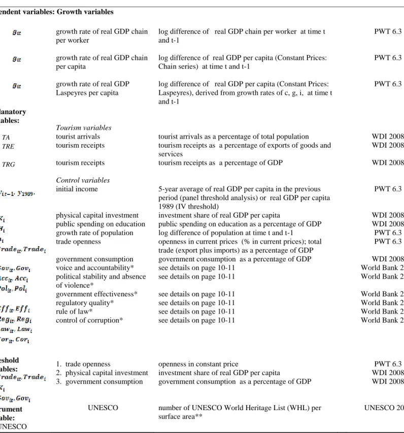
Economic growth is specified using the growth rates of three different GDP measurements, namely real GDP chain per worker (rgdpwok), real GDP chain per capita (rgdpch), and real GDP per capita (Constant Prices: Chain series), and real GDP Laspeyres per capita (rgdpl) or real GDP per capita (Constant Prices: Laspeyres), derived from the growth rates of c, g and i. These variables are obtained from the Penn World Tables version 6.3, which is available online at the Center for International Comparisons of Production, Income and Prices, University of Pennsylvania (see Heston et al. (2009)). Initial income is defined as the 5-year average of real GDP per capita in the previous period in the case of panel threshold analysis, and as the real GDP per capita in the initial year (1989) in the case of cross-sectional instrumental variable threshold analysis. This variable is used to capture the convergence process in the economic growth model.
The physical investment variable comes from the investment share of real GDP per capita (ki); population (POP), and openness in current prices (OPENK), which is total trade (the value of exports plus imports) as a percentage of GDP, and is used as a proxy for the trade openness variable. These are also obtained from the Penn World Tables version 6.3.
Public expenditure in education is used as a proxy for human capital, government consumption as a percentage of GDP, surface area (sq. km), and three tourism specialization variables, tourist arrivals, and tourism receipts as a share of exports of goods and services, tourism receipts as a share of exports of GDP, as an indication of the degree of tourism specialization, are obtained from the World Bank’s World Development Indicators (WDI) database.
For the institutional variables, we obtained the “Worldwide Governance Indicators (WGI) project” for 1996-2008 from the World Bank. It consists of six different indicators of institutional quality referring to six dimensions of governance, namely voice and accountability, political stability and absence of violence, government effectiveness, regulatory quality, rule of law, and control of corruption. These indicators are available biannually since 1996, and annually since 2002. In our analysis, the first available data (that is, 1996) are used for the values in the initial 5-year averaged period (1989-1993).
(1) Voice and accountability: captures perceptions of the extent to which a country’s citizens are able to participate in selecting their government, as well as freedom of expression, freedom of association, and a free media.
(2) Political stability and absence of violence: captures perceptions of the likelihood that the government will be destabilized or overthrown by unconstitutional or violent means, including politically-motivated violence and terrorism.
(3) Government effectiveness: captures perceptions of the quality of public services, the quality of the civil service and the degree of interdependence from political pressures, the quality of policy formation and implementation, and the credibility of the government’s commitment to such policies.
(4) Regulatory quality: captures perceptions of the ability of the government to formulate and implement sound policies and regulations that permit and promote private sector development.
(5) Rule of law: captures perceptions of the extent to which agents have confidence in and abide by the rules of society and, in particular, the quality of contract enforcement, property rights, the police and the courts, as well as the likelihood of crime and violence.
(6) Control of corruption: captures perceptions of the extent to which public power is exercised for private gain, including both petty and grand forms of corruption, as well as the impact on the state by the elite and private interests.
The UNESCO World Heritage List (WHL) per country is obtained from a website of UNESCO (http://whc.unesco.org/en/list). The World Heritage List includes 890 properties forming part of the cultural and natural heritage, which the World Heritage Committee considers as having outstanding universal value. This includes 689 cultural, 176 natural and 25 mixed properties in 148 States Parties. As of April 2009, 186 States Parties had ratified the World Heritage Convention. The details of the variables and data sources are provided in Table 3.
5. Empirical Specification 5.1 Panel Threshold Model
The main purpose of this paper is to use a threshold variable to investigate whether the relationship between tourism specialization and economic growth is different in each sample grouped on the basis of certain thresholds. This is to determine if the existence of threshold effects between two variables is different from the traditional approach, in which the threshold level is determined exogenously. If the threshold level is chosen arbitrarily, or is not determined within an empirical model, it is not possible to derive confidence intervals for the chosen threshold. The robustness of the results from the conventional approach is likely to be sensitive to the level of the threshold. The econometric estimator generated on the basis of exogenous sample splitting may also pose serious inferential problems (for further details, see Hansen (1999, 2000)).
The critical advantages of the endogenous threshold regression technique over the traditional approach are as follows: (1) it does not require any specified functional form of non-linearity, and the number and location of thresholds are endogenously determined by the data; and (2) asymptotic theory applies, which can be used to construct appropriate confidence intervals. A bootstrap method to assess the statistical significance of the threshold effect is also available in order to test the null hypothesis of a linear formulation against a threshold alternative.
For the reasons given above, we used the panel threshold regression method developed by Hansen (1999) to search for multiple regimes, and to test the threshold effect in the tourism and economic growth relationship within a 5-year panel data set. The possibility of endogenous sample separation, rather than imposing a priori an arbitrary classification scheme and the estimation of a threshold level, are allowed in the model. If a relationship exists between these two variables, the threshold model can identify the threshold level and permit testing of such a relationship over different regimes categorized by the threshold variable.
Although the Hansen (2000) approach is commonly used in cross-sectional analysis, it can also be extended to a fixed effect panel, provided that no endogenous problem exists.
Specifically, the method requires that all explanatory variables are exogenous. In some circumstances, especially in empirical growth models, the key variables for economic growth are likely to be endogenous. In an economic model, a variable is endogenous when there is a correlation between the variable and the error term. Endogeneity can arise as a result of measurement error, autoregression with auto correlated errors, simultaneity, omitted variables, and sample selection errors. The problem of endogeneity occurs when one or more regressors are correlated with the error term in a regression model, which implies that the regression coefficient in an OLS regression is biased. Thus, the Hansen (2000) approach will no longer be applicable. In order to overcome the endogeneity problem, instrumental variable estimation of the cross-sectional threshold model introduced by Caner and Hansen (2004) is also used.
Hansen (1999) developed econometric techniques appropriate for threshold regression with a panel data. Allowing for fixed individual effects, the panel threshold model divides the observations into two or more regimes, depending on whether each observation is above or below a threshold level. The observed data are from a balanced panel ( . The subscript i indexes the individual and t indexes time. The
dependent variable, , is scalar, the threshold variable is scalar, and the regressor is a k
vector. The structural equation of interest is
(13)
where I() is an indicator function.
The observations are divided into two regimes, depending on whether the threshold variable, , is smaller or larger than the threshold, . The regimes are distinguished by different regression slopes, and . For the identification of and , it is necessary that the elements of are not time-invariant. The threshold variable, , is not time invariant.
is the fixed individual effect, and the error is assumed to be independently and identically distributed (iid), with mean zero and finite variance .
The threshold value ( ) is estimated using the least squares method developed by Hansen (2000). A bootstrap procedure is used to obtain approximate critical values of the test
statistics which allows one to perform the hypothesis test for the threshold effect. If the bootstrap estimate of the asymptotic p-value is smaller than the desire critical value, then the null hypothesis of no threshold effect is rejected. After a threshold value is found, the confidence intervals for the threshold value and slope coefficients are then estimated. A similar procedure can also be conducted to deal with the case of multiple thresholds. The possibility of existence of more than one threshold represents another advantage of this method over the traditional approach.
Our focus is to assess the role of tourism specialization on economic growth. The economic growth regression based on the neoclassical growth model described in the previous session is augmented with the tourism variables in order to investigate empirically the relationship between tourism specialization and economic growth varies across subsamples grouped on the basis of various threshold variables. The empirical specification of the economic growth regression, with tourism specialization within the panel threshold model framework, is represented as follows:
(14)
where
) is the indicator function;
is the growth rate of real GDP chain per worker (rgdpwok). We also use different
definitions for income, namely real GDP chain per capita (rgdpch) and real GDP Laspeyres per capita (rgdpl) in order to check whether the result is robust to the different specifications of the real GDP growth rate;
is the tourism specialization variable that is widely used as a proxy for the
influence of international tourism in most empirical tourism studies. There are several alternatives to measure the volume of tourism discussed by Gunduz and Hatemi (2005). One is tourism receipts, which is the volume of earnings generated by foreign visitors, a second is the number of nights spent by visitors from abroad, and a third is the number of tourist arrivals. Depending on the availability of data for most countries in our sample, the second cannot be
considered. As a result, three measures of tourism are used to check whether the impact on economic growth is sensitive to different specifications of tourism measurement.
The selected tourism variables are as follows (Sequeira and Campos, 2007):
(1) tourist arrivals as population proportion (TA);
(2) tourism receipts as a share of exports of goods and services (TRE); (3) tourism receipts as a share of real GDP (TRG).
is the threshold variable used to examine whether tourism plays a different role in the
growth process due to the differing regimes endogenously categorized by three criteria, namely degree of trade openness ( ), investment share to GDP ( ), and the government
consumption expenditure as a percent of GDP ( ). These threshold variables are highly
related to international tourism policies. Specifically, the degree of trade openness could be used to capture the relevance of a country to international trade. Clearly, international tourism and international trade are two major sources of foreign currency for small, as well as larger economies. We use trade openness as the criteria to verify whether the impact of tourism specialization on economic growth differs across regimes. The investment share to GDP is also used as a threshold variable as investment is an important factor to support tourism expansion. The extent of government consumption involvement in the economy represents government-induced distortions. In our analysis, we consider whether the impact of tourism specialization at different levels of government-induced distortions different across countries.
represents the vector of other explanatory variables and control variables which are:
is the 5-year average of real GDP chain per worker for panel threshold analysis
(and real GDP chain per capita and real GDP Laspeyres per capita, depending on which specification is used as the dependent variable) from the previous period, which is used to capture the convergence process. It is also defined as the real GDP chain per worker (or real GDP chain per capita and real GDP Laspeyres per capita) in the initial year (1989) for instrumental variable threshold analysis (a negative sign is expected);
is the investment share of real GDP per capita, which is used as a proxy for physical
capital investment (a positive sign is expected);
is the stock of human capital (currently, a common proxy is the average years of
schooling in the population, but there might be a problem with this proxy due to excluding the quality of education: omitting the quality may decrease human capital accumulation, and bias the results, so we use an alternative proxy for human capital, which is public spending on education as a percentage of GDP, and can be used to capture the quality of education as well as human capital investment);
is the population growth rate (a negative sign is expected);
is trade openness in constant prices, which is used to measure the impact of
openness of the economy in its growth performance, and is consistent with the current emphasis on the export-led growth hypothesis (a positive sign is expected);
is the ratio of government consumption to GDP, which measures the extent of
government involvement in the economy, and can also capture the effects of distortions induced by government);
The six institutional variables used in the model are as follows:
is an indicator of voice and accountability;
is an indicator of political stability and absence of violence;
is an indicator of government effectiveness;
is an indicator of regulatory quality;
is an indicator of the rule of law;
The inclusion of institutional variables in empirical growth studies has recently been taken into consideration because the quality of institutions is regarded as a pre-condition to exploit natural and/or historical endowments which tourism development relies on (Brau et al., 2009); moreover, the inclusion of such an important explanatory variable identifies a further possible channel whereby tourism could affect economic growth through institutions (a positive impact is expected);
is the individual (country) effect, is a time effect, and is independently and
identically distributed across countries and years.
5.2 Instrumental Variables (IV) Threshold Model
Next, we briefly introduce the Instrumental Variable (IV) threshold model developed by Caner and Hansen (2004). This approach is carried out with the pure cross-sectional data averaged over 1989-2008, such that there is one observation per country.
The observed sample is , where is real valued, is a m-vector, and is a
k-vector, with . The threshold variable, , is an element or a function of the
vector , and must have a continuous distribution. The data are either a random sample or a
weakly dependent time series, so that unit roots and stochastic trends are excluded. The structural equation of interest is
which may also be written in the form
The threshold parameter is , where is a strict subset of the support of . This
parameter is assumed to be unknown and is to be estimated.
The reduced form is a model of the conditional expectation of , given :
where , and the parameter is unknown.
The reduced form threshold parameter, , may equal the threshold, , in the structural equation,
but this is not necessary, and this restriction will not be used in estimation. Caner and Hansen (2004) estimate the parameter sequentially. First, they estimate the reduced form parameter by
OLS. Second, they estimate the threshold, , using predicted values of the endogenous variable,
. Third, the slope parameters, and , are estimated by 2SLS or GMM on the split samples
implied by the estimate of .
It is widely perceived that the effect of tourism specialization on economic growth gives rise to the possibility of both endogeneity and thereby a reverse relationship. Unobservable variables such as managerial skills that are crucial inputs in tourism activities, could directly explain both high economic growth and a high level of tourism. Moreover, security and health issues, such as political stability, criminality and malaria, are detrimental to both tourism and growth (Arezki et al., 2009). We then apply instrumental variable estimation of a threshold model proposed by Caner and Hansen (2004) to avoid the endogeneity problem and to investigate the threshold effect of tourism specialization on economic growth. The IV threshold regression takes the form:
(16)
(17)
where ) is the indicator function, is the vector of keys variables which are , ,
, , , , , , , , , and is the threshold variable, which
( ) and the level of government consumption , is the number of the UNESCO
World Heritage List per surface area, which is an instrumental variable , is the threshold
value, and , and , are two sets of slope parameters corresponding to the low and high
regimes, respectively. Equation (17) is estimated using OLS by substituting the fitted values of the endogenous variable, , into (16). Then the threshold parameter, , is estimated using
OLS. Finally, the slope coefficients are estimated using GMM on the split samples.
6. Empirical Results
The main objective is to investigate the threshold effect of tourism specialization on economic growth by applying endogenous threshold regression techniques rather than arbitrarily assuming cut-off points through a theoretical specification within the panel and cross-sectional growth regression frameworks. In both frameworks, we select three key variables as threshold variables for tourism specialization and growth relationship. Specifically, the selected threshold variables are the degree of trade openness, investment share to GDP, and the government consumption expenditure as a percentage of GDP.
The robustness of the tourism specialization and growth relationships is checked by using different definitions of tourism specialization and the growth rate of real GDP per capita. Three tourism specialization definitions are used to quantify the impact of international tourism specialization on economic growth, namely tourist arrivals as a proportion of the population (TA), tourism receipts as a share of exports of goods and services (TRE), and tourism receipts as a share of real GDP (TRG). We also use various measurements of real GDP per capita, namely growth rate of real GDP chain per capita (rgdpch), growth rate of real GDP chain per worker (rgdpwok), and growth rate of real GDP (Laspeyres) per capita (rgdpl), which are obtained from the Penn World Table 6.3 (PWT).
6.1 Results from panel threshold regression
The descriptive statistics for the variables used in the 5-year panel threshold model are reported in Table 4. We first conduct the panel threshold analysis, in which the slope estimates of the tourism specialization variables switch between regimes over different thresholds. The
other variables are omitted as their coefficients do not change significantly from the linear specification model. Any results discussed in this section but not presented are available from the authors upon request.
[Insert Table 4 here]
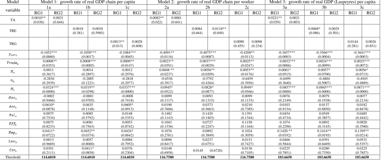
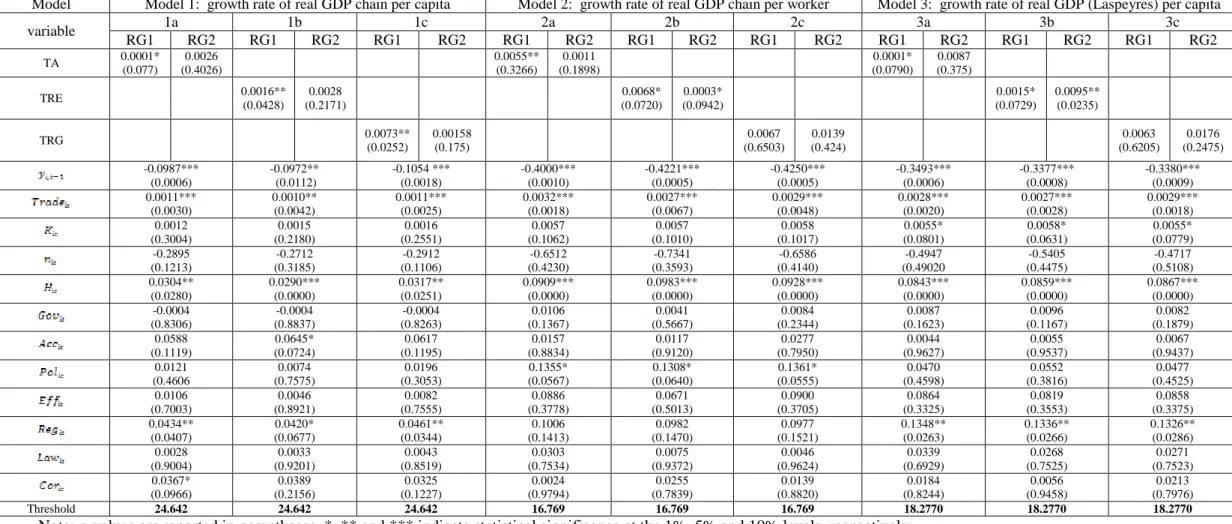
Before estimating the threshold regression model, we test for the existence of a threshold effect between economic growth and tourism. This paper uses the bootstrap method to approximate the F statistic, and then calculates the bootstrap p-value. The results are estimated over three economic growth specifications, with three different tourism specialization measures over three possible thresholds. The test statistic for a single threshold is significant for all models, while the test statistics for double and triple thresholds are insignificant. Thus, we may conclude that there is strong evidence that there is a single threshold in the relationship between economic growth and tourism within the 5-year panel data context. Given a single threshold effect between economic growth and tourism, the whole sample is split into two regimes, where three variables, namely degree of trade openness, investment share to GDP and government consumption as a percentage of GDP, are used as the threshold variables. When a threshold is found, a simple regression can be used to yield consistent estimates. The threshold regression estimates for the economic growth-tourism model, using the Hansen (2000) method, are reported in Tables 6, 7 and 8.
These three tables report the results from the threshold regression, where trade openness, investment share to GDP and government consumption are used as the threshold variables. The first conclusion to be drawn from Tables 6,7 and 8 is that the initial value of real GDP per capita is negative and statistically significant for all growth regressions for each possible threshold. The coefficients are not especially different across these three models. Moreover, the coefficients of initial income in models 1, 2 and 3 do not differ across three possible thresholds. The negative and significant effect of initial income is evidence of conditional convergence in the growth process, which predicts higher growth in response to a lower starting real GDP per capita, and the important influence on the growth rate (see Barro and Sala-i-Martin (2003)).
Second, the estimated coefficient of trade openness is found to be positive and significant for all regressions across the three threshold variables, which supports the positive influence of
trade on economic growth. Third, the investment share to GDP, which is a proxy for physical investment, has a positive effect on economic growth. Fourth, the population growth rate and government consumption are found to have negative effects on economic growth, but are not statistically significant in all regressions. Fifth, the coefficients of public investment in education are statistically significant and positive for most regressions over the three threshold variables. This finding is consistent with the literature on human capital and growth, which suggests that the accumulation of human capital can promote economic growth. Finally, the role of institutions, by introducing various measures of institutional quality, is found to be positive and significant for some regressions across the three thresholds. This confirms that a strong social infrastructure is influential in explaining the economic development process.
[Insert Tables 6, 7 and 8 here]
Focusing on the coefficients of tourism specialization, namely TA, TRE and TRG, the results for the three economic growth models indicate that there is a positive (and typically significant) relationship between tourism specialization and economic growth across three different economic growth specifications. The coefficients associated with tourism specialization are robust to different tourism specialization definitions in each growth model, and this is consistent with the different threshold variables. Tourism specialization alone plays an ambiguous role in contributing to economic growth for two regimes. The higher impact of tourism on economic growth is sometimes found in regimes 1 and 2.
6.2 Results from IV threshold regression
In order to examine the contribution of tourism specialization to economic growth with different thresholds and regimes, the potential endogeneity of the level of tourism specialization in the growth regression needs to be taken into account. Ignoring this issue can lead to biased estimates of the coefficient associated with tourism in the growth regression, in which several explanatory variables are likely to be endogenous. Therefore, we apply instrumental variable estimation of an endogenous threshold model, as recently developed by Caner and Hansen (2004), to the pure cross-sectional data averaged over 1989-2008. The possible threshold effect of tourism specialization on economic growth is estimated, while the endogeneity problem is
estimates of the slope parameters are obtained by using generalized method of moment (GMM). Following Arezki et al. (2009), the number of UNESCO sites for each country’s surface area is used as the instrumental variable. [In their study, the instrument for tourism is the number of UNESCO sites per 100,000 inhabitants in the year 2002, kilometers of coastal area, and related interactions as additional instruments. They further test the robustness of the results by using different versions of the UNESCO World Heritage List, and the number of sites per surface area is also included in their analysis.]
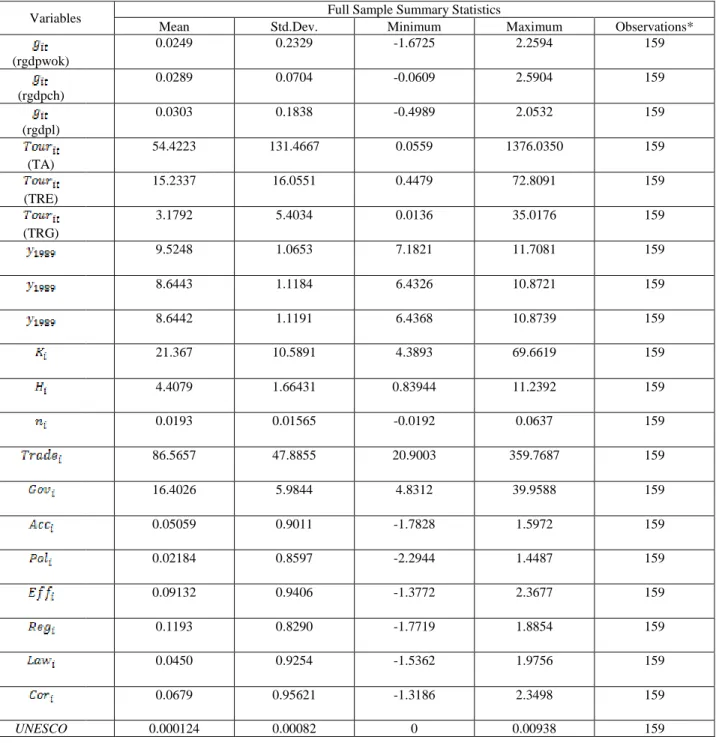
The descriptive statistics for the variables used in the cross-sectional IV threshold model are reported in Table 5. Tables 9, 10 and 11 report the results from the IV threshold model. Three different growth specifications, with three alternative measures of degree of tourism specialization, as well as the set of control variables in the economic growth literature, are investigated in the threshold effect of tourism specialization on economic growth. The two regimes are based on different threshold variables, namely the degree of trade openness, investment share to GDP, and government consumption as a percentage of GDP. In contrast to the panel threshold analysis in the previous session, the slope coefficients of the tourism variables, as well as other control variables, switch between regimes. We consider whether the coefficients of these key variables change between regimes after taking account of endogeneity in the cross-sectional regression.
[Insert Table 5 here]
Tables 9, 10 and 11 show the results from three different definitions of the economic growth regressions, namely growth rate of real GDP chain per capita (rgdpch), growth rate of real GDP chain per worker (rgdpwok), and growth rate of real GDP (Laspeyres) per capita (rgdpl). The whole sample is grouped by the degree of trade openness, the investment share to GDP, and the ratio of government consumption to GDP. In each table, regressions (1a)-(1c) are growth regressions of rgdpch augmented with three tourism variables, namely tourist arrivals as a proportion of population (TA), tourism receipts as a share of exports of goods and services (TRE), and tourism receipts as a share of real GDP (TRG), respectively. Regressions (2a)-(2c)
and (3a)-(3c) are organized in the same manner for the rgdpwok and rgdpl growth regressions, respectively.
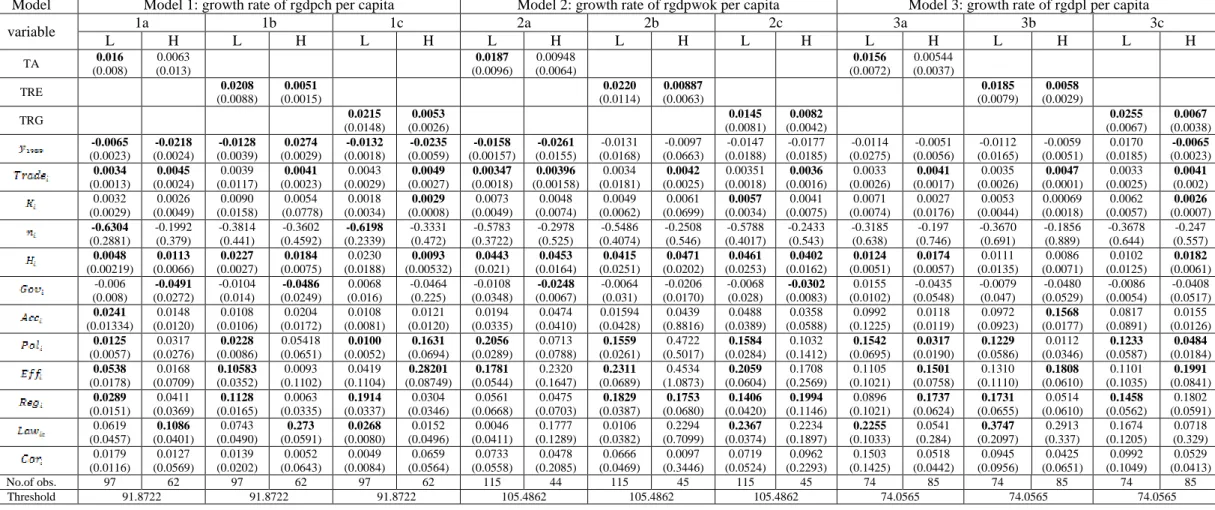
In Table 9, the threshold values for trade openness are as follows: 91.872 for the rgdpch per capita growth regression (model 1), where 97 countries have a smaller value and 62 countries have a larger value; 105.486 for the rgdpwok per capita growth regression (model 2), where 115 countries have a smaller value and 44 countries have a larger value; and 74.056 for
the rgdpl per capita growth regression (model 3), where 74 countries have a smaller value and
85 countries have a larger value.
The relationship between tourism specialization and economic growth is found empirically. The coefficients associated with the tourism development variables range from 0.0145 to 0.029 in the lower trade openness regime, from 0.0051 to 0.00948 in the higher trade openness regime, and are significant across different growth rate specifications. These results suggest that tourism development has a positive growth-boosting effect on the open economy, though this contribution may not be sustained as the economy reaches very high trade openness. According to Brau et al.(2009), who define a group of states with a degree of tourism specialization greater than 8%, on average, over the period 1980-2004 as tourism countries, the results here suggest that 33 countries can be characterized as “tourism countries”. Most of these tourism specialized countries have a degree of trade openness higher than the estimated threshold value for trade openness, particularly the small tourism specialized countries. About 41.07% (or 34.92%) of countries with trade openness greater than 105.49% (or 91.87%) are tourism countries. In other words, several countries with a relatively high degree of tourism specialization (tourism country) generally involve a higher degree of trade openness, yet they have not been able to achieve the desired consequences of this particular characteristic of economic growth.
The results obtained by Adamou and Clerides (2009) are supportive in this respect. They find that specialization in tourism adds to a country’s rate of economic growth, but it does so at a diminishing rate. This means that, at high levels of specialization the independent contribution of tourism to economic growth becomes minimal, and tourism can even become a hindrance to further growth. This interesting finding can be explained by the fact that the tourism destinations
support tourism expansion which, in turn, leads to a higher degree of trade openness. Furthermore, a sub-optimal use of natural resources of a country with relative endowment of natural resources might induce the country’s loss of comparative advantage in tourism with a lower contribution of tourism, and possibly also cause unsustainable economic growth in the long run.
The negative sign associated with initial income (the natural logarithm of real GDP per capita in 1989) supports the convergence hypothesis, some of which are significant. Regarding the influence of initial income on the growth rate, two estimation methods yield substantially different results. Such differences arise because initial income is measured differently based on alternative estimation methods. The initial income in a 5-year panel (a fixed effect panel), for instance, is defined as the 5-year average of income from the previous period. However, the initial income commonly used to check for convergence in the growth process in a pure cross-sectional analysis is income in the initial year. The difference in the coefficients of initial income in both methods emerges from differences in specification.
Trade openness provides evidence of the positive impact on economic growth. Note that the slightly greater magnitude is found in the higher-trade opening regime, which implies that the more open countries exert a powerful impact on economic prosperity. Investment share to GDP is found to be positive across all three models, but only a few are found to be statistically significant. The regressions also provide evidence of the negative impact of the population growth rate, the negative impact of government consumption, and the positive impact of six measures of institutional quality on economic growth. The coefficients of public investment in education for economic growth are found to be significantly positive for most regressions. This confirms that human capital plays a crucial role for economic growth, and that the inclusion of public expenditure in education in the economic growth regression is an accurate measure of human capital. The finding that human capital accumulation promotes economic growth is supported by several studies (see, for example, Barro (1991) and Barro and Lee (2001)).
Differences in the coefficients of the key variables between regimes are of particular interest. It is observed that the coefficients of all variables in the low regime are similar in
magnitude to those in the high regime for each corresponding economic growth specification. This empirical finding does not change as the threshold variable under consideration changes.
[Insert Table 9 here]
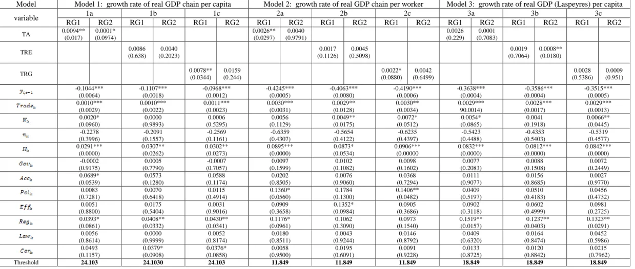
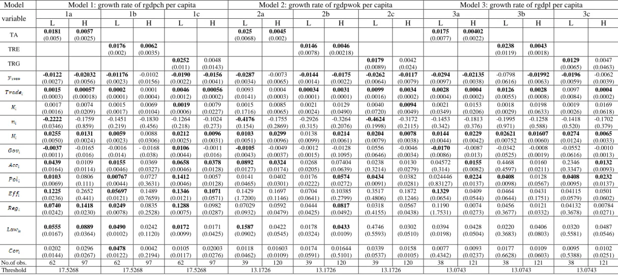
In Table 10, investment share to GDP is used as a threshold variable. The threshold values for the three growth specifications are similar. The threshold value for the rgdpch per capita growth regression (model 1) is 17.526, where 62 countries have a smaller value and 97 countries have a larger value; 13.1726 for the rgdpwok per capita growth regression (model 2), where 39 countries have a smaller value and 120 countries have a larger value; and 13.0743 for
the rgdpl per capita growth regression (model 3), where 38 countries have a smaller value and
121 countries have a larger value. The estimates in each model are in line with the economic growth literature. Initial GDP has the expected negative coefficient, and the magnitude is similar to those obtained from Table 9. With respect to the sign of the other coefficients, trade openness, investment share to GDP, and institutional variables have a positive impact on economic growth, while population growth and government consumption have a negative impact. As in Table 9, public investment in education typically has a positive impact on economic growth. It is observed that the coefficients of all variables in the low regime are similar in magnitude to those in the high regime for each corresponding economic growth specification.
The impact of tourism and economic growth seems consistent with the results in Table 9. The three tourism variables yield similar impacts on economic growth in each model. This implies that the impact of tourism specialization on economic growth is robust to the various specifications of tourism specialization. Although the significantly positive impact on economic growth is found, such impacts in different regimes are not the same. Tourism specialization has a slight effect on economic growth in the high-investment share countries, while the lower-investment share countries have a higher impact. The coefficients associated with the three tourism variables range from 0.0129 to 0.025 for the low-investment share regime, and from 0.00402 to 0.0062 for the high-investment share regime. Examining the list of countries with the investment share to GDP is greater than the estimated threshold value, it is found that 23.71%
(or 21.66%) of countries with investment share to GDP greater than 17.5268% (or 13.1726%), for example, are identified as “tourism countries”.
[Insert Table 10 here]
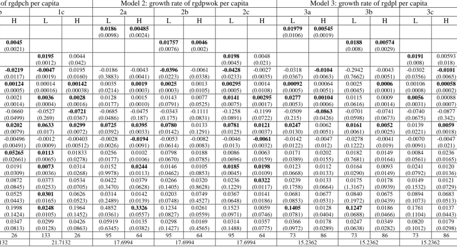
The results from three different growth specifications with government consumption expenditure as a percent of GDP as a threshold variable, are reported in Table 11. The crucial role of tourism expansion has been quantified through three different growth regressions. The empirical evidence from most regressions (a)-(c) in each economic growth specification strongly confirms the significantly positive impact of tourism specialization and economic growth. Only a few regressions are insignificant. The estimates of all three tourism effects range from 0.0175 to 0.0198 for the lower-government spending regime, and from 0.0044 to 0.00593 for the higher-government spending regime. All the tourism variables used to measure the reliance of a country on tourism yield similar findings for each empirical growth model.
Overall, the sign of the coefficients of the common regressors for economic growth are consistent with those reported in the previous tables. Moreover, similar magnitudes of the coefficients of all the variables across the two regimes in each corresponding economic growth specification are observed. In addition, it is found that government consumption has a largely negative impact in the high-government spending regime, while the low-government spending regime experiences lower negative impact on economic growth. This finding is of interest in the government spending and economic growth relationship. Economic theory does not automat-ically generate strong conclusions about the impact of government outlays on economic performance. Indeed, there are circumstances in which lower levels of government spending might enhance economic growth and other circumstances in which higher levels of government spending would be desirable.
The “Rahn Curve” measures the relationship between different levels of government spending and economic performance. The growth-maximizing point on the Rahn Curve is the subject of considerable research. Experts generally conclude that this point is somewhere between 15%-20% of GDP, although it is possible that these estimates are too high since
statistical studies are constrained by a lack of data for countries with limited governments (Larson, 2007). The threshold estimates for government spending in our case are 21.7132 for the
rgdpch per capita growth regression (model 1), 17.6995 for the rgdpwok per capita growth
regression (model 2), and 15.2363 for the rgdpl per capita growth regression (model 3). Therefore, countries in the high government-spending regime can be considered as countries where higher government spending leads to a lower growth performance.
[Insert Table 11 here]
7. Concluding Remarks
Tourism specialization has significant potential beneficial economic impacts on the overall economy of tourism destinations. This paper has not investigated the direction of the relationship between economic growth and tourism, but whether tourism specialization has the same impact on economic growth in countries that differ in their degree of trade openness, investment share to GDP, and government consumption as a percentage of GDP. In order to examine the contribution of tourism specialization to economic growth, the analysis is undertaken with different threshold variables and regimes through the panel threshold regression model of Hansen (2000) and IV threshold model of Caner and Hansen (2004). A 5-year averaged panel data set and a pure cross-sectional data set of 159 countries over the period 1989-2008 were used.
The results obtained from the panel threshold model of Hansen (2000) showed that economic growth is boosted by means of trade openness, investment share, public investment in education, and institutional variables, while population growth and government consumption have negative effects. Initial income, trade openness, and public investment in education are significant in most regressions, and this remains unchanged as the threshold variable changes. However, the degree of influence of tourism specialization on economic growth in different regimes does not hold for several regressions or for different threshold variables. As a result, there is no consensus regarding whether tourism specialization has the same impact on economic growth for different values of the threshold variables.
We applied instrumental variable estimation of a threshold regression approach, developed by Caner and Hansen (2004), to quantify the contributions of tourism specialization on economic growth, while correcting for endogeneity. The number of UNESCO World Heritage List per surface area is used as the instrumental variable. The results of the instrumental variable threshold estimation reveal thatthe estimates in each model are similar to those found in the economic growth literature. Initial GDP has the expected negative effect, implying the existence of conditional convergence in the economic growth process. Trade openness, investment share to GDP, and institutional variables have a positive impact on economic growth, while population growth and government consumption have a negative impact, and are insignificant in most regressions. Public investment in education typically has a positive impact on economic growth. It is observed that the coefficients of all variables in the low regime are similar in magnitude to those in the high regime for each corresponding economic growth specification. These empirical findings do not change as the threshold variable under consideration changes.
Focusing on the coefficients of tourism specialization, namely TA, TRE and TRG, the results for the three economic growth models indicate that there is a significant and positive relationship between tourism specialization and three economic growth specifications. The robustness of such a relationship is illustrated by the qualitatively unchanged direction of the coefficients associated with the tourism specialization variables. The significant impact of tourism specialization on economic growth in most regressions is robust to the different specifications of tourism specialization, as well as to the different real GDP measures. However, the coefficients of these tourism specialization variables in the two regimes are significantly different, with the higher impact of tourism on economic growth found in the lower regime. These findings do not change as the threshold variables under consideration change.
The greater reliance on tourism through three tourism specialization definitions increases the economic growth rate, but relatively less than that of the countries in the lower-trade openness regime or lower-investment regime. Countries with a higher degree of trade openness and investment are tourism countries. By listing countries with trade openness and investment share to GDP greater than the threshold values, about 41.07% with trade openness greater than 105.486%, and 23.71% with investment share to GDP greater than 17.5268%, are identified as