Volatility Forecasting An Empirical Study on Bitcoin Using Garch and Stochastic Volatility models

Volatility

Forecasting

An empirical study on bitcoin

using garch and stochastic volatility models

Author

Hugo Hultman

Peter Jochumzen

Abstract

Cryptocurrencies are on the rise, with new financial assets, new frameworks need to be developed. This thesis sets out to the examine the GARCH(1,1), the bivariate-BEKK(1,1), and the Standard stochastic volatility model’s volatil-ity forecasting performance on BTC/USD, where the bivariate model is esti-mated on both BTC/USD and ETH/USD closing price data. Furthermore, three loss functions are used to evaluate the forecast accuracy for each model. The functions are estimated using realized volatility based on BTC/USD data on a minute per minute basis. The result indicates that the GARCH(1,1) is the model that performs best regarding forecast accuracy. All three loss func-tions rank the models accordingly; first the GARCH(1,1), second the bivariate-BEKK(1,1), and finally the Stochastic volatility model.

Contents

4 Forecast Evaluation 11 4.1 Volatility proxy . . . 11 4.2 Loss functions . . . 13 5 Data 13 6 Results 14 6.1 Parameter Estimations . . . 15 6.2 Forecast Evaluation . . . 16 7 Analysis 19 8 Conclusion 20 8.1 Further Research . . . 20 9 References 21

1

Introduction

Being able to model and create accurate forecasts of financial volatility is crucial for risk management purposes, portfolio selections as well as for pricing financial instruments (Hull, 2011). Due to high demand for accurate volatility estimates the interest amongst researches has been tremendous. Volatility is a latent variable and cannot be observed. However, there are some features that are commonly observed in financial data. Financial time series data often exhibits periods of high volatility followed by periods of low volatility. Volatility also varies within a finite range and often evolves over time in a continuous manner (Tsay, 2002). The huge interest and many features of volatility have led to a vast universe of different type of volatility models. All aimed to catch these features and improve the accuracy of volatility prediction. According to Tsay (2002), volatility models can be divided into two subcategories, describing the evolution of volatility either as a deterministic process or as a stochastic process.

In this thesis, we examine models from both categories. We use three differ-ent volatility models; a GARCH(1,1), a Standard stochastic volatility model (SV-model), and a bivariate-BEKK(1,1). The GARCH model first proposed by Bollerslev (1986) has become a workhorse for volatility forecasting. The literature covering this model is extensive, and it has been applied to a variety of financial assets. See for example Andersen and Bollerslev (1998), Hansen and Lunde (2005), and Wang and Wu (2012). Andersen and Bollerslev’s findings suggest that both GARCH models and stochastic volatility models provide volatility estimates that are closely corre-lated with the future volatility. Hansen and Lunde do an extensive study using over 300 models from the ARCH model universe; their findings show no evidence of the GARCH(1,1) being outperformed by any of the more sophisticated models on exchange rates. Moreover, Wang and Wu compare forecast performance between univariate and multivariate GARCH type models. They use, amongst other models, a GARCH(1,1) and a full BEKK(1,1). To evaluate the models they use six different loss functions. Two which we use in our analysis, the Mean squared error (MSE) and Mean absolute error (MAE). While the majority of the loss criteria prefer the multi-variate over the unimulti-variate models, the MSE and MAE prefer the GARCH(1,1) over the full BEKK(1,1). Moreover, both Franses et al. (2008) and Boscher et al. (2000) compare the GARCH model and the SV-model on stock return data and interest rate data respectively. They both find evidence that the SV-model performs better than the GARCH model. However, this evidence is more distinct the in-sample than in the out-of-sample evaluation.

While the volatility literature is widespread and covers a variety of models as well as assets, the research on Bitcoin and cryptocurrencies, in general, is much

more limited. Corbet et al. (2018), investigate the dynamic relationships between cryptocurrencies and other financial assets. They include two of the larger cryp-tocurrencies in their study; Ripple and Lite coin. Their findings indicate that there exists a spillover effect on the cryptomarket, which implies that these three coins are interconnected, thus a reason to incorporate a bivariate model in our analysis. Furthermore, Dyhrberg (2016) employs a single GARCH model on Bitcoin data while other researchers like Katsiampa (2018) employ multiple GARCH models to compare and find a superior model. Katsiampa (2018) evaluates the volatility pre-dictions using a goodness of fit test. The paper includes a GARCH(1,1) model, however, the findings support an AR-CGARCH model in case of modeling Bitcoin data. Also, Salisu and Adediran (2018) investigate justification for time-varying stochastic volatility in Bitcoin returns. Their findings suggest that by modeling Bitcoin volatility using a stochastic model could lead to better forecast results than by ignoring the same.

There is no universal volatility model that is superior for all asset classes. With the rise of new cryptocurrencies, new frameworks need to be developed. The aim of this thesis is to provide daily volatility forecasting of Bitcoin/USD closing price data. The GARCH(1,1) and the SV-model are fitted on BTC/USD data, while the bivariate-BEKK(1,1) is fitted on both BTC/USD and ETH/USD closing price data. The data covers the period between 2015-08-06 and 2018-06-27, totaling 1057 daily observations. To produce one-step-ahead volatility forecasts, each model is estimated using a rolling window approach. The forecast horizon is 360 days covering the period between 2017-07-03 and 2018-06-27. Furthermore, to evaluate the forecast accuracy three different loss functions are used, all based on moments of forecast errors; the mean squared errors, root mean squared errors and mean absolute errors. These are estimated using realized volatility based on historical BTC/USD closing prices on a minute per minute basis, as a proxy for the true volatility process. The results indicate a very conclusive ranking amongst the models. According to the forecast evaluation, the GARCH(1,1) provides the most accurate forecast. All three loss functions prefer this model over the other two models and rank them in the same order; first GARCH(1,1); second bivariate-BEKK(1,1); and last the SV-model.

The remainder of this thesis is organized as follows. Section 2 gives the reader a brief introduction to Bitcoin. Section 3 presents the theory and methodology used throughout this thesis. Furthermore, section 4 presents the loss functions and the volatility proxy used in this thesis. Section 5 presents the data and section 6 the empirical results. Finally, in section 7 and 8 we analyze the results and summarize and conclude respectively.

2

Bitcoin

The following description of Bitcoin and Blockchain is based on Antonopoulos (2008). In 2008 an individual or group of programmers under the pseudonym Satoshi Nakamoto proposed Bitcoin as a "peer-to-peer electronic cash system"; a digital pay-ment system that was completely decentralized without any authority. It was the birth of the first successful digital coin. Since the initialization of Bitcoin, there has been a major boom of new digital coins. Bitcoin is also a cryptocurrency which means that it uses cryptography to make it secure. What separates Bitcoin from the traditional currencies is that it only exist in digital units, unlike the more common paper currencies. The usage of Bitcoin is multifaceted; it can be used as almost any other currency, it can be used to buy and sell goods as well as send money to individuals and organizations. It is often bought and sold on specialized exchanges where it can be exchanged for traditional currencies (Böhme et al., 2015). However, researchers have been arguing on how to classify Bitcoin; as an asset or as a cur-rency (Dyhrberg, 2016). Whelan (2013) argues that there are similarities to the US dollar, where the biggest difference is the decentralization. Furthermore, according to Glaser et al. (2014), a majority invest in Bitcoin for financial speculation rather than use it as a payment. Bitcoin does however present risks that are not associ-ated with the more traditional payment methods (Böhme et al.,2015). They argue that users are exposed to market risk due to volatility between Bitcoin and other exchange rates. Moreover, users also face transaction risk, due to the reason that the Bitcoin payments are final, and the system provides no support for reversing unwanted transactions (Böhme et al., 2015).

Before the birth of Bitcoin, there have been many attempts to establish a digital currency. Major obstacles have amongst others been to prevent counterfeits and dou-ble spending, i.e., spending a single coin more than once, as the Bitcoin technology successfully solves. Bitcoin builds upon a pioneering technology called Blockchain. Blockchain consists of chains of blocks of information. To break it down this infor-mation consists mostly of transactions. One could say that Blockchain is a digital ledger that contains all previous transactions (Tapscott and Tapscott, 2016). The average block consists of 500 transactions, and once a block is formed and verified, it is added to the chain. Each block in the chain are identified by a hash-algorithm or put in another way a digital fingerprint and contains the previous block’s hash. This block is referred to as the parent block. Every block has only one parent block, and together they form a chain. By modifying the parent block it will produce a new hash, since the blocks are interconnected, it will force the child to change, and so on. If the chain is long, this process requires heavy computer power which makes the transaction history hard to manipulate and is a main characteristic of the

Blockchain. The easiest way to buy Bitcoin is by doing so on a crypto-exchange. The users commonly store their coins in a Bitcoin wallet. The Bitcoin wallet is a database or a file and contains keys which allow the users to prove ownership of the transaction in the Bitcoin network. Each collection of key pairs consists of a public key and a private key. Where the public key can be compared to your bank account number and the private key as your private pin-code. The private key is usually picked random, and from that, the public key is derived. Further, the Bitcoin ad-dress is generated from the public key. This adad-dress is used as an identifier when sending Bitcoins to another person and is unique for each transaction. Moreover, the public key is used to receive Bitcoins while the private key is used for signing transactions.

Everything in the Bitcoin system is built to support one thing; transactions. A transaction is to put simply, just a transfer of value between two participants. The life cycle of a transaction starts with a request for transferring value from one owner to another. Before the transaction is finalized and included in the Blockchain, it needs to be verified. As mentioned above, a feature that separates the traditional conventional currencies from the Bitcoin is that there is no authority ensuring trust. Instead, this trust is ensured by its participants. In case of a transaction, the owner of the Bitcoins shows their public key and their signature. Since blockchain is a public ledger, the transaction is announced to the whole Bitcoin network and not only to the receiving part. In this way, all users in the Bitcoin network can confirm that the transaction is valid by confirming that the one is pursuing this transaction owns the coins. The participants validate and propagate the transaction until it reaches a mining node. The mining node creates blocks of transactions which must be valid. Their purpose is to sort transactions in a meaningful manner as well as creating new coins. This is done by a proof-of-work procedure, which means that a difficult problem needs to be solved to verify the transaction. When enough transactions are verified, they constitute a block, and if satisfying the requirements, the block is added to the chain. As compensation, the miners receive a fee for each transaction as well as the opportunity to be rewarded Bitcoins for the new coins introduced. Furthermore, the Bitcoin algorithm tightly controls the supply flow of new Bitcoins. The algorithm is programmed to create a problem every ten minutes. The speed of the production is controlled by changing the difficulty of the problem to solve. The supply is predicted to have reached it’s culmination 2040 when the maximum supply of Bitcoin 21m is achieved. After that, there will be no further possibility to produce Bitcoins.

3

Volatility Models

In this section, we introduce the three time-series models used in this thesis, describe essential theoretical background as well as the procedure to obtain the results.

3.1

GARCH(1,1)

Following Bollerslev (1986) we define the GARCH(1,1) in the following way: Letεt be a discrete-time stochastic variable andFtbe the information set of all information through time t. A GARCH(1,1) process is then given by

εt|Ft−1 ∼ N(µ, ht) (1)

ht=α0+α1ε2t−1+βht−1 (2) The GARCH(1,1) describes the conditional variance, ht, at time t, as a function of the previous period’s squared sample variances, ε2

t−1, and the previous period’s conditional variance, ht−1. α0 is a constant term, α1 capture the effect of ε2t−1, the ARCH effect, and β captures the effect of ht−1, the GARCH effect. We define the conditional volatility as √ht ≡ σt. Furthermore, to guarantee that the condi-tional variance ht is non-negative and stationary the following restrictions need to be satisfied:

α0 >0, α1 ≥0 β ≥0, α1+β <1.

Estimating the GARCH(1,1) model

Letytdenote price at timet, t = 1,. . .,T. We assume that the price can be described by an log-AR(1) process

logyt=φlogyt−1+εt, (3) next,to obtain the obtainεt we do the following

logyt=φlogyt−1+εt→εt= logyt−φlogyt−1.

A common method to use to estimate the parameters in the GARCH model is the maximum likelihood method. The first step in this procedure is to form a likelihood function and the second step is to maximize this function; in order to obtain the parameter estimates. To form the likelihood function we are required to make a dis-tributional assumption about the data. Recall from equation 1 that we assume that

εt is normal distributed with mean µand variance ht. With use of this information we can derive the likelihood function. Letf(yt|Ft−1)denote the normal conditional probability density function and θ be a K × 1 vector of parameters. We can con-struct the joint density function f(y1, y2, .., yT;θ) as the products of the marginal density functions: f(y1, y2, ..., yT;θ) =f(yT|Ft−1)×f(yT−1|Ft−2)×. . .×f(y1). The likelihood functionL(θ|yT, ..., y1)is the same function as the joint probability func-tion with a slightly difference, we view it as a funcfunc-tion of the parameters given the set of data rather than opposite. For simplicity we consider the log-likelihood function instead denoted`(θ) .

`(θ) =−T 2 log(2π)− 1 2 T X t=1 loght− 1 2 T X t=1 yt−φyt−1 ht (4)

Also,h0 is unknown and has to be specified. A common choice forh0 which is used in this thesis is the unconditional sample variance (Zivot, 2009).

h0 = 1 T T X t=1 ε2_t

Next, we maximize the log-likelihood function. This optimization procedure is done in the R-language (R Core Team, 2018) using the standard function Optim. We use a rolling window approach to obtain the one-step ahead estimations updating the parameters daily, i.e. dropping the first observation and adding a new one as moving forward in time until reaching the end of the forecast horizon.

3.2

Bivariate-BEKK

Financial markets are often interconnected; thus price movements in one market can affect other markets (Tsay, 2002). It is therefore of high interest to model the volatility in Bitcoin by account for interdependency between other cryptocurrencies. To improve our volatility forecast, we include data of one of the larger cryptocur-rencies, Ethereum. The BEKK model is a multivariate GARCH model and was proposed by Engle and Kroner’s (1995). This type of model is used to explain how the covariances change over time. In the bivariate case the model can be represented in the following way: Let yt denote a 2 × 1 vector of prices, further, let εt be a 2

×1 vector of error terms, and Ft be the information set of all information through time t. Assume,

logyt = logyt−1 +εt (5)

Ht =CTC+ " a11 a21 a12 a22 # " ε2_1,t−1 ε1,t−1ε2,t−1 ε2,t−1ε1,t−1 ε22,t−1 # " a11 a12 a21 a22 # + " b11 b21 b12 b22 # Ht−1 " b11 b12 b21 b22 # (7) Where,Ht is a 2× 2 positive definite variance-covariance matrix and Cis a 2 × 2 lower triangular matrix such that C’C is assured to be semi-positive definite. The off-diagonal elements in matrix A2×2 = ai,j and B2×2 = bi,j , i,j=1,2, has a direct interpretation of cross market spillover effects (Lunina, 2016). However, the sign of these parameters are hard to make inference about. Since, they are encapsulating the effect of several non-linear variables (Lunina, 2016).

The parameter estimation of the BEKK is usually done by a maximum likelihood algorithm. By assuming that the innovations belong to a multivariate normal dis-tribution, we can construct the log-likelihood function denoted by

logLT(εT. . . ε1;θ) =− 1 2 " T N log(2π) + T X t=1 (log|Ht|+εtH−t1εt # (8)

Each parameter estimate is obtained by maximizing equation 8. However, compared to the GARCH(1,1) the maximum likelihood estimation in multivariate time-series models is much more complex which makes the estimation non-trivial (Francq and Zakoian, 2015). As the number of variables increases the number of parameters be-comes large and obtaining convergence can be difficult (Francq and Zakoian, 2015). In this thesis, the estimation is done in the R language (R Core Team, 2018) using the packageMTS(Tsay, 2015). Initial values forh0,bitcoinandh0,ethereumneeds to be chosen. In line with the GARCH(1,1) model, we use the unconditional sample vari-ance as starting values for the conditional varivari-ance. To estimate the parameters we use a rolling window. However, unlike the other two other models, the parameters in the bivariate-BEKK is only updated every ten days due to the time-consuming estimation process. As we move towards time T, we drop the first observation in the data sets and add ten new until we reach the end of the forecast horizon.

3.3

The standard stochastic volatility model

As an alternative approach to the GARCH-models we introduce a new class of volatility models; Stochastic volatility models. Stochastic volatility is a common concept used in financial economics to deal with time-varying components (Shep-hard, 2005). According to Platanioti et al. (2005), an economic motivation to use a stochastic model is to provide greater flexibility in describing stylized facts of finan-cial time series data. Referring to heavy tails and leverage effect are arguments to use such a model. The difference between the GARCH models and the SV-model

is that the latter assumes that the conditional variance evolves from a stochastic process.

The standard stochastic volatility model is a time-discrete stochastic model, initially introduced by Taylor (1982). Let yt denote price at time t, t = 1,. . .,T. Then the SV-model can be described as follows

yt= exp(ht/2)εt, with εt∼ N(0,1) ht=µ+φ(ht−1−µ) +σηηt, with ηt∼ N(0,1) h0 ∼ N(µ, σ_η2 1−φ2) (9)

Whereεtandηtare independent white noise processes,ht≡logσt2and the initial stateh0 is drawn from the stationary distribution of the AR(1) process. Unlike the GARCH models, a feature of the SV-model is that the processytis assumed to have its "own" contemporary variance (Kastner, 2016). This variance is only allowed to vary in a finite range over time, and thus we assume it’s the logarithm that follows an AR(1) process. Moreover, there are three parameters in the SV-model that needs to be estimated, θ = [φ, µ, ση]T. φ can be interpreted as the persistence in the volatility and to guarantee thatht is a stationary process the model requires |φ| <1. Furthermore, µ and ση can be referred to as the level of the log-volatility and the volatility of the log - volatility. Finally, ht is an unobserved latent process and is often referred to as the time-varying volatility process, and it can be interpreted as the random flow of new information in the financial market (Platanioti.et.al, 2005).

Estimating the Standard SV-model

While the GARCH(1,1) model easily can be estimated by MLE, a major drawback with the SV-model is that its likelihood function is not tractable and requires nu-merical methods to evaluate and the estimation procedure becomes therefore non-trivial. In this thesis, we use the package Stochvol (Kastner, 2016) from the R language (R Core Team, 2018) in order to estimate the parameters. The package uses a Markov-Chain Monte Carlo method to estimate the parameters. The MCMC method relies on the Bayesian approach and has become a very popular method to estimate the SV-model (Platanioti.et.al, 2005). Unlike the frequential school, the Bayesian school treats the unknown parameters θK×1 as a random variable. The distribution of θ is known as the prior and incorporates the prior beliefs we have about the parameters. Hence, the first step is to choose a prior, i.e. make a distri-butional assumption about the parameters θ = [µ, φ, ση]T. The prior distribution, p(θ), in theStochvolpackage is accordingly to Kim.et al (1998) using independent components for each parameter, i.e. p(θ) = p(µ)p(φ)p(ση). It employs a normal

prior for the level µ ∈ R with the hyperparameters bµ and Bµ, for the persistence φ∈ (−1,1), a beta distribution with hyperparameters a0 and b0. For the volatility of the log variance ση ∈ R+ , the Stochvol package assumes ±

p

σ2

η to follow a centered normal distribution with hyperparameter Bση

µ∼ N(bµ, Bµ)

(φ+ 1)/2∼β(a0, b0)

±qσ2

η ∼ N(0, Bση)

(10)

Choosing a good prior is not easy and requires careful thinking. Kastner (2016) suggest that to choose a non-informative prior, i.e., pick a prior such that a small change in the prior does not affect the results too much, there are some good options forµandσ_η2but choosingφ, however, is harder. Since the choice of the variance forµ andσ2

η does not influence the result very much as long as we pick them large enough. ForµKastner (2016) suggest setting the hyperparameters very vague, i.e., choose a low mean and large variance. Hence, our choice for this parameter isµ∼ N(0,100). For σ2

η we are accordingly to Kastner (2016) choosing ±

p

σ2

η ∼ N(0,1) not to be too small and use the default option in the package. Moreover, for the persistence parameterφ ∈(−1,1)we assume (φ+ 1)/2∼β(5,1.15) which is the default option and implies a prior mean about 0.54 with std of 0.31.

After specifying the prior beliefs, we run the MCMC sampler provided in the

Stochvol package to obtain the draws from the posterior joint distribution of the parameters. The prior distribution can be seen as the distribution; we believe the parameters follow before seeing the data. The posterior distribution can be seen as the belief of the parameters post using the data. Unlike the maximum likelihood method, the MCMC output does not provide a best fit but instead a parameter distribution. Hence, leaving us the choice to select a value that we consider best in some sense. To obtain our estimates, we use a rolling window approach. We update the parameters each day, by moving the window one step ahead while dropping the first observation and adding a new one until we reach the end of the forecast horizon. We then pick the mean in each posterior as a point estimate used to produce the future volatility estimates.

4

Forecast Evaluation

4.1

Volatility proxy

A question that comes to mind in case of evaluating the forecast is that the variable of interest σt is a latent variable, which means that it cannot be observed. The

importance of a "good" proxy for the latent volatility is, therefore, crucial to be able to evaluate forecast accuracy. A common practice has been to estimate the true volatility using the sample standard deviation (Poon & Granger, 2003).

ˆ σt= 1 N −1 N X t=1 (Rt−R¯)2

This proxy, however, is not entirely satisfactory while using small samples sizes (Poon and Granger, 2003). Another common practice is to use daily squared returns calculated from daily closing prices as a proxy for the true volatility. While squared returns are an unbiased estimator of the volatility and hence can be justified, it turns out that it is an extremely noisy estimator which may lead to poor forecast results. Moreover, some research has also used absolute squared returns as a proxy for the true volatility. See for example Ghysels et al. (2006).

A solution to this problem is suggested by Andersen and Bollerslev (1998). They suggest an alternative proxy, realized volatility, based on intra-day returns as a less noisy proxy compared to squared returns. This has become a popular practice in finance (Poon and Granger, 2003). We define the discretely observed series of continuously compounded returns with m observations per day as

r(m),t+j/m = log (pt+j/m)−log (pt+(j−1)/m), j = 1, . . . , m (11) where, the realized volatility can be computed by

ˆ σ2_(m),t := m X j=1 r2_(m),t+j/m ˆ σ(m),t = q ˆ σ2 (m),t (12)

There is a clear theoretical motivation behind using this proxy, since it is an unbiased estimator of the true volatility. See for example Barndorff-Nielsen and Shephard (2002), and Andersen et al. (2003). Moreover, Andersen and Bollerslev (1998) shows that the forecasting performance for GARCH models increases while using intraday data compared to interday data. Since, it is a less noisy proxy compared to squared returns based on interday data (Andersen and Bollerslev, 1998). Hence, this thesis use realized volatility based on intraday data as a proxy for the true volatility process to evaluate the forecast accuracy.

4.2

Loss functions

Being able to measure the forecast accuracy is fundamental to inference the volatility forecast. There exist several methods for measuring this quantity. Since some functions are more suited for some purposes, the choice should depend upon the forecast purpose (Lee, 2007). A common approach to evaluate forecast accuracy is to use a function which measures the forecast error. In our case, this error describes the difference between the true volatility and the estimated volatility. According to Granger (1999), there are three properties a loss function is required to satisfy. Let et denote the forecast error at time and f(et) be an arbitrary loss function. Then it must satisfy the following, i) f(0) = 0, if there is no error there will be no loss, ii) min f(et) = 0 s.t f(et)≥0 and that f(et) is monotonic non-decreasing as the error moves away from zero. Common functions to use for time-series volatility evaluation are amongst other the Mean Square Error (MSE), Root Mean Square Error (RMSE) and Mean Absolute Error (Poon and Granger, 2003).

In this thesis we use the MSE ,RMSE, and MAE to evaluate the forecast accuracy.

M SE:L( ˆσt, σt) = 1 T T X t=1 ( ˆσt−σt)2 (13) M AE :L( ˆσt, σt) = T X t=1 |σˆt−σt| (14) RM SE :L( ˆσt, σt) = s PT t=1( ˆσt−σt) T (15)

According to Patton (2011) the MSE is a robust loss function no matter what proxy are used for the latent volatility. Furthermore, Vilhelmsson (2006) argues that the MSE is sensitive to outliers while MAE is robust to this event. However, worth to keep in mind is that the actual expected loss is greater while using a proxy than by using the true volatility (Patton, 2011).

5

Data

The data examined in this thesis consist of three data sets. The data sets used for estimating the volatility models consists of daily closing prices in BTC/USD and ETH/USD. These two data sets are collected from Yahoo Finance, and the samples consist of 1057 observations spanning between 2015-08-06 and 2018-06-27. The forecast horizon is 360 days which spans between 2017-07-03 and 2018-06-27. The third sample consists of historical BTC/USD closing prices on a minute per minute

basis collected from Kaggle. This data sample is used to construct the volatility proxy. The sample consists of totally 525 600 observations. Below in figure 1 we can see the BTC/USD and ETH/USD price evolution between 2015-08-06 and 2018-06-27. Moreover, in table 1 we find sample statistics for BTC/USD and ETH/USD.

Figure 1: Daily closing prices in Bitcoin/USD and Ethereum/USD between 2015-08-06 and 2018-06-27

Table 1: Descriptive statistics for BTC/USD and ETH/USD

N = 1057 Min Max Mean sd Kurtosis Skewness BTC/USD 211.43 19345.49 3162.9 4017.88 1.8 1.58 ETH/USD 0.42 1385.02 201.89 290.97 1.65 1.54

6

Results

This section presents the estimates from the parameter estimations as well as the performance results from the loss functions. As described earlier a rolling window approach is used and the parameters in the GARCH(1,1) and SV-model are updated each day, whereas the bivariate-BEKK(1,1) is updated each ten days. This yields 360 estimates per parameter for the GARCH(1,1) and the SV-model, and 36 estimates per parameter for the BEKK(1,1). Due to the large number of parameters we choose to present the maximum, minimum and median parameter estimate for each model.

6.1

Parameter Estimations

GARCH(1,1)

Table 2 presents the parameter estimates from the GARCH(1,1) model. The first parameter φ comes from equation 3. Table 1 implies that all the 360 estimates for φ take the value one. Furthermore, the parameter α0 which denotes the constant term in the GARCH equation, has a maximum of 0.0012, a minimum of 1.0000e-03, and a median of 1.0000e-03. Where a significant majority of the estimates comprises 1.0000e-03. Moreover, α1, also called the ARCH-parameter, reflects how much the past residuals affect the current volatility. We can see that the maximum, the minimum, and the median estimates are 1, 0.2019, and 0.2810 respectively. The parameter β, which captures the GARCH effect in the model, i.e., measures what impact previous volatility have on future volatility, indicates a maximum, minimum and median estimate of 0.3354,1.0000e-03, and 0.1130 respectively. This implies that the ARCH effect on average has a larger impact on the future volatility than the GARCH effect for this data set.

Table 2: The maximum,minimum and median parameter estimation for the GARCH(1,1). The statistics are obtained from the sample of daily parameter estimates covering the fore-cast horizon 2017-08-03 and 2018-06-27.

φ α0 α1 β

Max 1 0.0012 1 0.3354 Min 1 1.0000e-03 0.2019 1.0000e-03 Median 1 1.0000e-03 0.2810 0.1130

Bivariate-BEKK

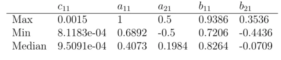
The parameter estimates in table 3 concern the bivariate BEKK(1,1). As in the previous model, the estimates are obtained by using a rolling window approach. A total of 36 estimates per parameter are obtained. Table 3 shows the maximum, minimum and median estimate for each parameter. Since this thesis aims to model the volatility in Bitcoin, we do only present the parameters that are contained in the conditional variance of Bitcoin in equation 7.

The parameterc11 which represents the constant term in this model, has a maxi-mum, minimaxi-mum, and median estimate of 0.0015, 8.1183e-04, and 9.5091e-04 respec-tively. The parameters a11 and a21 captures the effect of ε21,t−1 and ε1,t−1ε2,t−1. The results indicate that the maximum parameter estimate takes on the value 1, the minimum 0.6892 while the median is 0.4073. Furthermore, a21 has a maximum of 0.5, a minimum of -0.5 and a median of 0.1984. The last two parameters b11 and b21 measures the effect from the past volatility. b11 shows a maximum estimate of 0.9386, a minimum of -04436, and a median of 0.8264. By comparing b21 to b11

we see that b11 has a lower maximum and a negative median. As mentioned in section 3, the off-diagonal elements can be interpreted as a measure of cross-market volatility spillover effect and are hard to make inference about. Hence, we cannot draw any conclusion about the signs of this parameters. Neither can we conclude if spillover effects are present since we do not investigate the significance level of the off-diagonal elements.

Table 3: The maximum, minimum and median parameter estimation for the bivariate-BEKK(1,1). The statistics are obtained from the sample of the parameter estimates for the bivariate-BEKK(1,1) covering the forecast horizon 2017-08-03 and 2018-06-27.

c11 a11 a21 b11 b21 Max 0.0015 1 0.5 0.9386 0.3536 Min 8.1183e-04 0.6892 -0.5 0.7206 -0.4436 Median 9.5091e-04 0.4073 0.1984 0.8264 -0.0709

SV-model

In table 4 we find parameter estimates for the standard stochastic volatility model. The statistics presented in the table are computed from a sample of 360 observations per parameter. The results indicate that all the parameters satisfy their respective parameter constraints. For the constant term µ we can see that it takes on a negative value for all the 360 estimates. The largest value it takes on is -5.9754 and the smallest -8.4126. The persistence parameterφ takes on values in the range between 0.9763 and 0.7148, with a median value of 0.9197. This implies that the previous period’s volatility has quite a high impact on the one-step-ahead volatility. The last parameter ση, also interpreted as the volatility of the log-volatility and encapsulate the effect of the stochastic element takes on values between 0.3420 and 1.1455 with a median of 0.5931.

Table 4: The maximum, minimum and median parameter estimation for the SV-model. The statistics are obtained from the sample of daily parameter estimates covering the forecast horizon 2017-08-03 and 2018-06-27. µ φ ση Max -5.9754 0.9763 1.1455 Min -8.4126 0.7148 0.3420 Median -7.4599 0.9197 0.6196

6.2

Forecast Evaluation

In this section, the error statistics from the forecasts are presented, and the predicted volatility from the three models are plotted against the realized volatility. In table 5, we find the error statistics from the three loss functions. The results from the

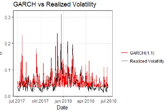
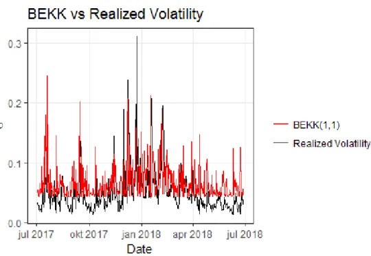
loss functions indicate that the GARCH(1,1) is the model that has performed best according to the proxy used. All three loss functions rank the models consistently, first the GARCH(1,1) model, secondly the Bivariate-BEKK and finally the SV-model. By looking at figure 2 we can get a better overlook how the GARCH(1,1) model has performed over the forecast horizon period. Furthermore, figure 3 shows how the BEKK(1,1) has performed compared to the volatility proxy and figure 4 tells us how the SV-model has performed according to the volatility proxy.

Table 5: Error statistics for the GARCH(1,1), bivariate-BEKK(1,1), and SV-model

MAE RMSE MSE GARCH(1,1) 0.0232 0.0340 0.0012 BEKK(1,1) 0.0322 0.0466 0.0022 SV-Model 0.0477 0.0737 0.0054

Comparing figure 2 and figure 3, it seems like the GARCH(1,1) and BEKK(1,1) produce very similar volatility results. It seems like the most distinct difference is in the period covering October and the period covering April to July, where the GARCH(1,1) seems to follow the Realized volatility more closely. The SV-model in figure 4 produces less noisy results. It does not seem to capture the essence of the true volatility very well but instead performing a random walk over the period. Furthermore, figure 4 indicates that the SV-model seems to capture very little of the fluctuations around December-January, where the volatility was very high.

Figure 2: Estimated Bitcoin volatilty from the GARCH(1,1) to Realized volatility covering 2017-07-03 to 2018-06-27

Figure 3: Estimated Bitcoin volatilty from the bivariate-BEKK(1,1) to Realized volatility covering 2017-07-03 to 2018-06-27

Figure 4: Estimated Bitcoin volatilty from the SV-model to Realized volatility covering 2017-07-03 to 2018-06-27

7

Analysis

As described in the previous section, the results indicate that the GARCH(1,1) forecast ability is superior to the other models. All three loss functions rank the models in the same order. Franses et al. (2008) and Boscher et al. (2000) suggest the SV model in favor of the traditional GARCH(1,1). Also, Salisu and Adediran (2018) finds that by including a stochastic component one could improve their result while modeling Bitcoin returns. This is not in line with our findings, where the SV-model shows the poorest performance out of the three SV-models. While an argument for using the SV-model is that it is more in line with modern financial theory. A reason for the poor performance could be that, since we are working with parametric models, it is the parameters that capture all the information there is to know about the data. The MCMC output gives us a distribution over each parameter and since we only use the mean of this distribution as the parameter estimate. There is a possibility that we exclude important information that could have generated better results regarding forecast accuracy. Also, the impact of starting values for the initial volatility estimate may play a role. While a common choice is to use the unconditional sample variance as the first volatility estimate and which is used in both the GARCH and the BEKK model. The SV-model assumes that the initial volatility is drawn from the stationary distribution ofht and evolves from that.

Wang and Wu (2012) compares seven volatility model and are using eight differ-ent loss criteria to evaluate the out of sample forecast on the energy market, amongst others MAE and MSE. The models they evaluate are amongst others a GARCH(1,1) and a BEKK(1,1). Their findings are in line with our results. Both the MAE and MSE prefers the GARCH(1,1) model over the bivariate-BEKK. Corbet et al. (2018) find evidence of interdependency between Bitcoin, Ripple and Lite coin. The effect of including Ethereum in our model is not easily interpreted since the sign of the off-diagonal elements are hard to make inference about, since they do capture the ef-fect of several non-linear terms. Moreover, to be able to tell if cross-market spillover effects are present we do need to know if the parameters are significant. This is how-ever excluded in the analysis due to a large number of parameter estimates. Another argument why the GARCH model provides better accuracy than the BEKK model could be that the parameters in the GARCH model are updated daily compared to the BEKK which are updated every ten days. This implies that the GARCH model quicker absorbs new information regarding the data than the BEKK model. It is plausible that this may play a role since the Bitcoin price exhibits large price movements according to figure 1.

8

Conclusion

We have compared three types of volatility models regarding their ability to fore-cast the one-day-ahead volatility in Bitcoin. The models used are a GARCH(1,1), a bivariate-BEKK(1,1) and a stochastic volatility model. The models are estimated using a rolling window approach. The parameters in the GARCH(1,1) and the Stochastic volatility model are updated each day, whereas the parameters in the BEKK(1,1) are updated every ten days. To evaluate the forecast accuracy, we use three different loss criteria, the MAE, MSE, and RMSE. These are constructed us-ing realized volatility as the estimate of the unobserved true volatility. The main findings are that the GARCH model seems to outperform the other model and that the SV-model is inferior to the other two models. While the loss functions are con-sistent in their ranking, it is, however, worth to keep in mind that use of statistical loss functions is subject to a proxy for an unobservable process.

8.1

Further Research

There are many ways to extend this study. We could:

• Extend the BEKK model by including other cryptocurrencies or assets than Ethereum. The same could be done for the SV-model to investigate if the forecast performance could be improved.

• Since financial time series data often exhibit heavier tails than the normal distribution. An interesting extension could be to estimate the models under a distribution that accounts for this feature.

• Further extension could also be to use different priors, initial values or up-date the parameters in the bivariate-BEKK(1,1) each day in order to seek improvement regarding forecast accuracy.

9

References

[1] Andersen, Torben. G. & Bollerslev, Tim. (1998). Answering the skeptics: Yes, standard volatility models do provide accurate forecasts. International Economic Review, 39(4), pp. 885-905.

[2] Andersen,Torben.G., Bollerslev,Tim., Diebold,Francis.X. & Labys, Paul. (2003). MODELING AND FORECASTING REALIZED VOLATILITY.Econometrica, 71(2), pp. 579-625

[3] Antonopoulos, Andreas.M. (2014).Mastering Bitcoin: Unlocking Digital Crypto-Currencies. (1st ed.) California: O’Reilly Media Inc.

[4] Barndorff-Nielsen,Ole.E. & Shephard, Neil.(2002). Econometric Analysis of Real-ized Volatility and its use in estimating stochastic volatility.J.R.Statistic.Soc.B, 64(B), pp. 253-280.

[5] Bollerslev, Tim. (1986). Generalized Autoregressive Conditional Heteroscedas-ticity. Journal of Econometrics, 31, pp. 307-327.

[6] Boscher, Hans., Fronk, Eva-Maria. & Pigeot,Iris. (2000). Forecasting interest rates volatilities by GARCH(1,1) and stochastic volatility models. Statistical Papers, 41, pp. 409-422.

[7] Böhme, Rainer., Christin,Nicolas., Edelman, Benjamin. & Moore,Tyler. (2015). Bitcoin: Economics, Technology, and Governance.Journal of Economic Perspec-tives, 29(2), pp. 213-238.

[8] Corbet, Shaen., Meegan, Andrew., Larkin, Charles., Lucey, Brian.& Yarovaya, Larisa.(2018). Exploring the dynamic relationships between cryptocurrencies and other financial assets. Economics Letters,165, pp.28-34.

[9] Dyhrberg Haubo, Anne. (2016). Bitcoin, gold and the dollar - A GARCH volatil-ity analysis. Finance Reasearch Letters, 16, pp. 85-92.

[10] Engle, Robert F. & Kroner, Kenneth F. (1995). Multivariate Simultaneous Generalized Arch.Econometric Theory, 11(1) , pp. 122-150.

[11] Francq, Christian. & Zakoian,Jean-Michel. (2015). Estimating multivariate volatility models equation by equation.Journal of the Royal Statistical Society, 78(3), pp. 613-635.

[12] Franses, Philip Hans., Van Der Leij, Marco. & Paap, Richard. (2008). A Simple test for GARCH Against a Stochastic Volatility Model. Journal of Financial Econometrics, 6(3), pp. 291-306.

[13] Ghysels, Eric.,Santa-Clara,Pedro. & Valkanov,Rossen. (2006). Predicting volatility:getting the most out of return data sample at different frequencies. Journal of Econometrics, 131, pp. 59-95.

[14] Glaser, Florian., Zimmermann, Kai., Haferkorn, Martin., Weber, Moritz Chris-tian. & Siering, Michael. (2014). Bitcoin - Asset or Currency? Revealing Users’ Hidden Intentions. In: Twenty Second Conference on Information Systems, ECIS 2014, (Tel Aviv). pp. 1-14.

[15] Granger, Clive.W. J.(1999). Outline of forecast theory using generalized cost functions.Spanish Economic Reqview, 1, pp. 161-173.

[16] Hansen, Peter & Lunde, Asger. (2005). A Forecast Comparison of Volatility Models: Does Anything Beat a GARCH (1,1)?.Journal of Applied Econometrics, 20, pp. 873-889.

[17] Hull, John. C. (2011).Options, Futures and Other Derivatives. (8th ed.). New Jersey: Pearson Education.

[18] Kastner,Gregor. (2016). Dealing with Stochastic Volatility in Time Series Using the R Package stochvol. Journal of Statistical Software, 69(5), pp. 1-30.

[19] Katsiampa, Paraskevi. (2018). An Empirical Investigation of Volatility Dynamics in the Cryptocurrency Market. SRN Electronic Journal. doi: 10.2139/ssrn.3202317.

[20] Kim, Sangjoon., Shephard, Neil. & Chib, Siddhartha. (1998).Stochastic Volatil-ity: Likelihood Inference and Comparison with ARCH Models. The Review of Economic Studies, 65(3), pp. 361-393.

[21] Lee, T.-H. (2007). Loss functions in time series forecasting. In International Encyclopedia of the Social Science (2nd ed.). Farmington Hills, Mich.: Macmillan Reference USA.

[22] Lunina, Veronika. (2016). Multivariate modelling of Energy Markets.Lund Eco-nomics Series, 39, Lund: Department of EcoEco-nomics, Lund University.

[23] Patton, A.J. (2011). Volatility forecast comparison using imperfect volatility proxies.Journal of Econometrics, 160. pp. 246-256.

[24] Platanioti,K., McCoy,J. & Stephens,D,A. (2005). A Review of Stochastic Volatility: univariate and multivariate models. Imperial College London.

[25] Poon, Ser-Huang. & Granger, Clive.W. J. (2003). Forecasting Volatility in Fi-nancial Markets: A Review.Journal of Economic Literature, 41(2), pp. 478-539.

[26] R Core Team. (2018).R: A language and environment for statistical computing. R Foundation for Statistical Computing, Vienna, Austria. URL: https://www.R-project.org/.

[27] Salisu, A, Afees. & Adediran. A, Idris. (2018). Testing for time-varying stochas-tic volatility in Bitcoin returns. Centre for Econometric and Allied Research, University of Ibadan Working Papers Series.

[28] Shephard, Neil. 2005. Stochastic volatility:Selected Readings. Oxford:Oxford University Press.

[29] Tapscott,Alex. & Tapscott, Don. (2016).Blockchain Revolution: How the Tech-nology Behind BITCOIN and Other CRYPTOCURRENCIES Is Changing the World. (1st ed.) New York:Portfolio/Penguin.

[30] Taylor, Stephen.J. (1982). Financial returns modelled by the product of two stochastic processes - a study of daily sugar prices 1961-79. In O.D. Ander-son(Ed.), Time Series Analysis: Theory and Practice, 1, pp. 203.226. Amster-dam: North-Holland.

[31] Tsay, Ruey. S. (2002).Analysis of Financial Time Series. (1st ed.). New Jersey: John Wiley & Sons Inc.

[32] Tsay, Ruey. S. (2015). MTS: All-purpose Toolkit for Analyzing Multivariate Time Series (MTS and Estimating Multivariate Volatility Models. R Package version 0.33. URL: https://CRAN.R-project.org/package=MTS.

[33] Vilhelmsson, Anders. (2006). Garch Forecasting Performance under Different Distribution Assumptions.Journal of Forecasting, 25, pp.561-578.

[34] Wang, Yudong. & Wu, Chongfeng. (2012). Forecasting energy market volatility using GARCH models: Can multivariate models beat univariate models?.Energy Economics,34(6), pp. 2167–2181.

[35] Whelan, K. (2013). How is bitcoin different from the dollar? Forbes. Novem-ber 19th. URL: http://www.forbes.com/sites/karlwhelan/2013/11/19/ how- is-bitcoin- different- from- the- dollar/. (Collected: 2018-08-22)

[36] Zivot, Eric. (2009).Practical Issues in the Analysis of Univariate GARCH Mod-els.In: Andersen, T. G., R. A. Davis, J. Kreib, and T. Mikosch (ed.). Handbook of Financial Time Series. Heidelberg: Springer-Verlag, pp. 113-155.