Learning to Propagate Labels on Graphs: An Iterative
1Multitask Regression Framework for Semi-supervised
2Hyperspectral Dimensionality Reduction
3Danfeng Honga,b, Naoto Yokoyac, Jocelyn Chanussotd, Jian Xua, Xiao Xiang Zhua,b 4
aRemote Sensing Technology Institute (IMF), German Aerospace Center (DLR), Wessling, Germany 5 bSignal Processing in Earth Observation (SiPEO), Technical University of Munich (TUM), Munich, 6
Germany 7
cGeoinformatics Unit, RIKEN Center for Advanced Intelligence Project (AIP), RIKEN, Tokyo, Japan 8 dUniv. Grenoble Alpes, CNRS, Grenoble INP, GIPSA-lab, Grenoble, France 9
Abstract 10
Hyperspectral dimensionality reduction (HDR), an important preprocessing step prior to high-level data analysis, has been garnering growing attention in the remote sensing community. Although a variety of methods, both unsupervised and supervised models, have been proposed for this task, yet the discriminative ability in feature representa-tion still remains limited due to the lack of a powerful tool that effectively exploits the labeled and unlabeled data in the HDR process. A semi-supervised HDR approach, called iterative multitask regression (IMR), is proposed in this paper to address this need. IMR aims at learning a low-dimensional subspace by jointly considering the labeled and unlabeled data, and also bridging the learned subspace with two regres-sion tasks: labels and pseudo-labels initialized by a given classifier. More significantly, IMR dynamically propagates the labels on a learnable graph and progressively refines pseudo-labels, yielding a well-conditioned feedback system. Experiments conducted on three widely-used hyperspectral image datasets demonstrate that the dimension-reduced features learned by the proposed IMR framework with respect to classifica-tion or recogniclassifica-tion accuracy are superior to those of related state-of-the-art HDR ap-proaches.
Keywords: Dimensionality reduction, graph learning, hyperspectral image, iterative, 11
1. Introduction 13
Recently, hyperspectral imaging in sensing techniques has garnered growing
at-14
tention for many remote sensing tasks [1], such as land-use and land-cover
classifica-15
tion [2, 3, 4], large-scale urban or agriculture mapping [5, 6, 7, 8], spectral unmixing
16
[9, 10, 11, 12], object detection [13, 14, 15, 16], and multimodal scene interpretation
17
[17, 18, 19, 20], as forthcoming spaceborne spectroscopy imaging satellites (e.g.,
En-18
MAP [21]) make hyperspectral imagery (HSI) available on a larger scale. Although
19
HSI features richer spectral information than RGB [22] and multispectral (MS) data
20
[23], yielding more accurate and discriminative detection and identification of
un-21
known materials, yet the very high dimensionality in HSI also introduces some crucial
22
drawbacks that need to be taken seriously: high storage cost, information redundancy,
23
and the performance degradation resulting fromthe curse of dimensionality, to name a
24
few. A general but effective solution to these issues isdimensionality reduction, also
25
referred to assubspace learning. In this process, we expect to compress the HSI to a
26
low-dimensional subspace along the spectral dimension while preserving the highest
27
possible spectral discrimination.
28
With the significant support in both theory and practice as well as a fact that
29
the learning-based strategy is somehow superior to the manually-designed feature
ex-30
traction [24], a considerable number of subspace learning approaches have been
de-31
signed and applied to hyperspectral data processing and analysis in the past decades
32
[25, 26, 27, 28, 29, 30, 31], particularly hyperspectral dimensionality reduction (HDR)
33
[32, 33, 34] and spectral band selection [35, 36]. Depending on their different
learn-34
ing strategies, HDR techniques are roughly categorized as unsupervised, supervised,
35
or semi-supervised strategies.
36
The classic principal component analysis (PCA) [37] is a user-friendly
dimension-37
ality reduction method for that is limited to capturing the underlying topology of the
38
data. Rather, manifold learning techniques (e.g., locally linear embedding (LLE) [38],
39
Laplacian eigenmaps (LE) [39], local tangent space alignment (LTSA) [40], and their
40
variants: locality preserving projections (LPP) [41], neighborhood preserving
embed-41
ding (NPE) [42], large-scale LLE [43], enhanced-local tangent space alignment
LTSA) [44]), by and large, follow the graph embedding framework presented in [45]. 43
This framework starts with the construction of graph (topology) structure and aim at 44
learning a low-dimensional data embedding while preserving the topological struc- 45
ture. Some popular and advanced methods have been proposed based on the graph 46
embedding framework for HDR. For example, Ma et al. [46] proposed to locally em- 47
bed the intrinsic structure of the hyperspectral data into a low-dimensional subspace 48
for hyperspectral image classification. Li et al. [47] modeled the locally neighboring 49
relations between hyperspectral data in a linearized system for HDR. In [48], a multi- 50
feature manifold discriminant analysis was developed on the basis of graph embedding 51
framework for hyperspectral image classification. Authors of [49] upgraded the exist- 52
ing landmark isometric mapping approach for the fast and nonlinear HDR. The same 53
investigators [50] further extended their work to linearly extract the low-dimensional 54
representation with sparse and low-rank attribute embeddings for HSI classification. In 55
[33], a joint spatial-spectral manifold embedding is developed to extract the discrimi- 56
native dimension-reduced features. Subsequently, Huang et al. [51] proposed a general 57
spatial-spectral manifold learning framework to reduce the dimension of hyperspectral 58
imagery. 59
In supervised HDR strategies, the main consideration is the discrimination between 60
intra-class and inter-class, where different discriminative rules are followed: local dis- 61
criminative analysis (LDA) [37], local fisher discriminative analysis (LFDA) [52], 62
sparse discriminant analysis [26], noise-adjusted discriminant analysis [53], feature 63
space discriminant analysis [54], and so on. Despite the superior class separability, 64
these methods still might fail to robustly represent the features due to sensitivity to var- 65
ious complex noises and ill-conditioned statistical assumptions, especially in the case 66
of small-scale samples. Unlike the aforementioned approaches that seek to project 67
the original data directly into a discriminative subspace, Ji et al. [55] simultaneously 68
performed dimensionality reduction and classification under a regression-based frame- 69
work, in order to find an optimally latent subspace where the decision boundary is 70
expected to be better determined. With the local manifold regularization in the pro- 71
jected subspace, this strategy has been successfully applied and extended to learn the 72
Most previously-proposed HDR methods adhere to either the unsupervised or the
74
supervised strategy, yet the labeled and unlabeled information is less frequently taken
75
into consideration. A straightforward way to consider the unlabeled samples is the
76
graph-based label propagation (GLP) [57], which has been successfully applied to
77
semi-supervised HSI classification [58] together with the support vector machine (SVM)
78
classifier. To effectively improve the discrimination and generalization of
dimension-79
reduced features, some proposed semi-supervised HDR works have been proposed by
80
the attempt to preserve the potentially global data structure that lies in the whole
high-81
dimensional space. For example, [59] followed a graph-based semi-supervised learning
82
paradigm for HDR and classification, where the graphs are constructed by different
lo-83
cal manifold learning approaches. A general but effective work integrating LDA with
84
LPP, called semi-supervised local discriminant analysis (SELD), was proposed in [60]
85
for a semi-supervised hyperspectral feature extraction.Inspired by GLP, [61] enhanced
86
the performance of LDA by jointly utilizing the labels and “soft-labels” predicted by
87
GLP for the semi-supervised subspace dimensionality reduction. Wu et al. [62]
pro-88
posed a similar approach to achieving a semi-supervised discriminative dimensionality
89
reduction of HSI by embedding pseudo-labels (instead of the similarity measurement
90
in LPP [60]) into LFDA rather than LDA in [61].
91
1.1. Motivation and Objectives
92
Although these proposed semi-supervised approaches have been proven to be
ef-93
fective in handling the issue of HDR to some extent, yet their graph structures for
94
unlabeled samples are constructed either from the similarity measurement (e.g., using
95
RBF) or from the pseudo-labels inferred by GLP or pre-trained classifier. The resulting
96
features by using this type of graph construction strategy is neither robust nor
gener-97
alized, due to the noisy data and labels as well as the scarce labeled samples. Also,
98
these semi-supervised algorithms, as often as not, attempt to find a single
transforma-99
tion that connects the original data and the subspace to be estimated. On account of
100
the complexity in the learning process, the optimal subspace search is hardly
accom-101
plished only by a single transformation. On the other hand, in spite of being guided
the learned subspace and the label space in the subspace learning strategy interpreted 104
by a single projection, further causing the performance bottleneck. In addition, these 105
subspace-learning-based models are commonly treated as a disjunct feature learning 106
step before classification. In other words, it is unknown what kinds of features in the 107
learning process may be capable of improving classification accuracy. 108
According to these factors, our objectives in this paper can be summarized as fol- 109
lows: 1) to bridge the to-be-estimated subspace with the label information more explic- 110
itly and effectively; 2) to introduce many unlabeled samples for improving the model’s 111
generalization ability; 3) and to refine the quality of class indicators of unlabeled sam- 112
ples for high discriminative HDR. 113
1.2. Method Overview and Contributions 114
Towards the aforementioned goals, a novel regression-induced learning model mo- 115
tivated by the joint learning (JL) framework [55, 56] is proposed, which seeks to learn 116
an optimal subspace by considering the correspondences between the training samples 117
and labels on a to-be-estimated latent subspace. We further extend the JL framework 118
to a multitask regression model with the joint embedding of labeled and unlabeled 119
samples. In the multitask framework, we also propose to adaptively learn asoft-graph 120
structure from the data rather than utilizing ahard-graph (fixed graph) constructed 121
manually or generated by additional algorithms, yielding a high-performance and more 122
generalized label propagation. In the meantime, to facilitate the use of pseudo-labels 123
more effectively, the learned graph can be updated after each outer iteration ends, and 124
the pseudo-labels accordingly refined, thereby enabling the learned features to be pro- 125
gressively optimized. More specifically, the main contributions of this work can be 126
highlighted as follows. 127
• We propose a JL-based variant: a novel iterative multitask regression (IMR) 128
framework by simultaneously considering few labeled samples and unlabeled 129
samples in quantity, with the application to semi-supervised HDR. 130
• We adaptively learn the connectivity (graph structure) between samples by align- 131
iterative 1 ... iterative t ... iterative n
Final Subspace Features Input HSI
t-step Subspace Features
Labeled HSI
Unlabeled HSI
S A
A:Regression Matrix Subspace Features
Subspace Features Labels
Pseudo-labels(t) Pseudo-labels(t+1) Learned Graph (t) (t) LP LP: Label Propagation Graph Learning S: Subspace Projection
Multitask Regression in t-step
... ...
(t) (t)
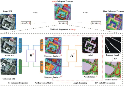
Figure 1: An overview of the proposed IMR framework. In fact, each iterative (t-step) starts with the input
of labeled and unlabeled data and ends up the output of the subspace projections (S(t)), regression matrix
(A(t)), and learned graph (W(t)) aligning the labeled with unlabeled samples. With thet-steplearned
graph, the pseudo-labels (t+ 1) can be refined.
• We deeply integrate the adaptive graph learning with the proposed multitask
re-133
gression framework in an iterative manner, making it possible for pseudo-labels
134
to be gradually updated using the learned graph in each outer iteration.
135
• We also design a general solver that originates from the alternating direction
136
method of multipliers (ADMM) optimizer for the solution of our proposed IMR
137
method.
138
2. The Proposed Methodology 139
In this section, we start with a brief review of our model’s cornerstone, the JL
140
framework, and then extend it to a variant of multitask learning by synchronously
re-141
gressing the labeled and unlabeled data. We will further introduce the proposed
iter-142
ative multitask regression (IMR) model by integrating the JL framework with the
ADMM-based optimizer is used for the IMR solution. Fig. 1 illustrates the workflow 145
of the proposed IMR method. 146
2.1. Review of the JL Model 147
LetXl ∈Rd×N be the unfolded hyperspectral data withdbands byN pixels (or 148
samples), andYl ∈Rl×N be the corresponding one-hot encoded label matrix withl 149
classes byNpixels. We model the original JL problem [55] as follows. 150
min A,S 1 2kYl−ASXlk 2 F+ α 2kAk 2 F s.t. SS T =I, (1)
whereS∈Rdsub×N andA∈
Rl×dsubdenote the subspace projection and the regres- 151 sion matrix linking the estimated subspace with label information, respectively, and 152
dsubrepresents the subspace dimension. || • ||Fdenotes the Frobenius norm andαis 153
the regularization parameter . 154
Slightly different from the original JL, an improved model with manifold (graph) 155
regularization is formulated by optimizing the following objective function. 156
min A,S 1 2kYl−ASXlk 2 F+ α 2kAk 2 F+ β 2 tr(SXlLlX T lS T) s.t. SST=I, (2)
whereLl∈RN×N =Dl−Wlis the Laplacian matrix,Wl∈RN×N is an adjacency 157
matrix (graph), andDl(ii)= Pi6=jWL(i,j)is the corresponding degree matrix. The 158
termtrdenotes the trace of matrix parameterized byβ. The JL-based models in Eqs. 159
(1) and (2) have been proven to be effectively solved with the ADMM optimizer [63]. 160
Once the projection matrixSis learned, the subspace features can be computed bySX. 161
2.2. Iterative Multitask Regression (IMR) 162
Labeling inEarth Vision is extremely costly and time-consuming, as the remote 163
sensing images have a larger-scale and more complex visual field. This leads to a lim- 164
ited number of labeled samples, which further hinders improvement of the model’s 165
learning and generalization capability. To this end, we effectively utilize the informa- 166
tion of unlabeled samples that are largely available by making a regression between the 167
W
L
Labeled Samples Unlabeled Samples
Lab el ed S amp le s U n lab el ed S amp le s
W
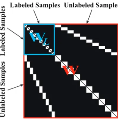
Figure 2: A showcase for joint adjacency matrix (W) (inred), whereWL(inblue) is a LDA-like graph
constructed by labels.
2.2.1. Multitask Regression with Graph Learning
169
In the multitask framework, we propose a learning-based graph regularization
in-170
stead of a fixed graph artificially constructed with the known kernels (e.g., using
Gaus-171
sian kernel function), in order to depict the connectivity (or similarity) between
sam-172
ples. Accordingly, a multitask regression framework is proposed for semi-supervised
173
HDR by optimizing the following objective function.
174 min A,S,L γ 2kYl−ASXlk 2 F+ 1−γ 2 kYpl−ASXplk 2 F+ α 2kAk 2 F +β 2tr(SXLX TST) s.t. SST=I, L=LT, Li,j,i6=j0, Li,j,i=j 0, tr(L) =s , (3)
whereXpl∈Rd×M andYpl∈Rl×M denote unlabeled hyperspectral data and a
one-175
hot encoded pseudo-label matrix, respectively, whileX = [Xl, Xpl] ∈ Rd×(N+M)
176
andL∈R(N+M)×(N+M)is a joint Laplacian matrix. The terms >0is a constant to
177
control the scale. Furthermore, the two fidelity terms in multitask learning are balanced
178
by a penalty parameterγ.
179
To solve (3) effectively, we rewrite the trace term as
180
tr(SXLXTST) = 1
2tr(WZ) = 1
in red). InW, the similarities betweenXcan be measured by apair-wise distance 182
matrix(Z∈R(2N+M)×(2N+M)) on Euclidean space; this matrix can be computed by 183 Zi,j =k(SX)i−(SX)jk2. Moreover, the operatoris interpreted as aterm-wise 184
Schur-Hadamardproduct. 185
By means of Eq. (4), optimizing problem (3) on a smooth manifold can be equiva- 186
lently converted on a sparse graph as follows. 187
min A,S,W γ 2kYl−ASXlk 2 F+ 1−γ 2 kYpl−ASXplk 2 F+ α 2kAk 2 F+ β 4kWZk1,1 s.t. SST=I, W=WT, Wi,j 0, kWk1,1=s . (5) In Eq. (5), thekWZk1,1is specified as apoint-wise weighted`1-normwith respect 188
to the variable ofW, yielding a weighted sparsity. 189
2.2.2. Optimizing Pseudo-Labels with Graph-based Label Propagation 190
In Eq. (3), the pseudo-labels are predicted by using a trained classifier, e.g., SVM 191
or random forest. Although the model’s performance can be moderately improved 192
through the use of unlabeled samples and pseudo-labels, yet the discrimination of 193
the dimension-reduced HSI still remains limited by only regressing the static pseudo- 194
labels. For this reason, the labels are dynamically propagated on the learned graph 195
using GLP, when the model converges in each step1, aiming at iteratively refining or 196
optimizing pseudo-labels, as illustrated in Fig. 1. The updated pseudo-labels together 197
with the other inputs ofXl,Xpl, andYlcan be re-fed into the next round of model 198
training, thus progressively improving the learning and generalization ability of the 199
proposed multitask model. 200
2.3. Modal Learning 201
Unlike the previous HDR methods following the graph embedding framework [46, 202
49, 33, 48, 51] that solve low-dimensional embedding as a problem of generalized 203
eigenvalues decomposition (GED) [45], our model learning process is to iteratively and 204
1Given the inputs ofX
landXplas well asYlandYpl, we estimate the variables ofA,S, andLby
Algorithm 1:Iterative Multitask Regression (IMR)
Input:Yl,Xl,Xpl,L,maxIter, and regularization parametersα,β,γ.
Output:A,S,L, andYpl
1 t= 1,ζ= 1e−4,= 1e−6,Obj = 1 +ζ; 2 InitializingAt,St,Wt, andYtpl
3 whileObj≥ort≤maxIterdo
4 k= 1,ObjIn= 1 +ζ;
5 whileObjIn≥ζori≤maxIterdo
6 Fix others to updateAk .Learning Regression Matrix
7 Fix others to updateSk .Learning Subspace Projections
8 Fix others to wisely updateWkinstead of directly optimizingLk
9 1. computeWk .Graph Learning
10 2. construct the LDA-like graph (WkL) for the labeled samples 11 3. replace the part ofWklearned by the labeled samples withWkL 12 4. obtainLk =Dk−Wk, whereDkii=Pi6=jWijk
13 Check the convergence condition of the inner loop:ifthe condition is satisfiedthen 14 Stop iteration; 15 OutputWt=Wk, Ztl=SkXl, Ztpl=SkXpl; 16 else 17 k←k+ 1; 18 end 19 end
20 UpdateYt+1pl withYtl,Ztl,Yplt,Ztpl,Wtusing LP .Updating Pseudo-labels 21 Check the convergence condition of the outer loop:ifWt==Wt−1or
Obj=kWt−Wt−1k F then 22 Optimization finished. 23 else 24 t←t+ 1; 25 end 26 end
alternately optimize several convex subproblems with respect to the variablesA,S, and
205
Was well as to-be-updatedYplinstead of directly solving the non-convex problem 206
(5) by the separable strategy of the variables. An implementation of the proposed
207
IMR is summarized inAlgorithm 1. Such optimization strategy has been proven to
208
be effective for solving the aforementioned issue [64, 65] and successfully applied in
209
many real cases [55, 56, 63, 66].
? ? ? ? ? ? ? ? 1 2 1 1 1 1 1 1 2 2 2 2 ... 1 1 1 1 2 2 2 2 2 2
Label Propagation in Feature Space
Yl(t) Ypl(t) Zl(t) Zpl(t) W(t) Ypl(t+1) ... ...
Figure 3: An illustration of label propagation used for updating the pseudo-labels, whereZ(lt)=S(t)X
land Z(plt)=S(t)X
pldenote the low-dimensional feature representation for the labeled and unlabeled samples,
respectively.
2.3.1. Learning Regression Matrix (A) 211
Intuitively, the optimization problem for solving the variable Ais a Tikhonov- 212
regularized least square regression, which is formulated as follows. 213
min A γ 2kYl−ASXlk 2 F+ 1−γ 2 kYpl−ASXplk 2 F+ α 2kAk 2 F. (6)
A closed-form solution of Eq. (6) is given by 214
A= (γYlHl+ (1−γ)YplHpl)×(γHlHTl + (1−γ)HplHTpl+αI)−
1, (7)
whereHl=SXlandHpl=SXpl. 215
2.3.2. Learning Subspace Projections (S) 216
The variableScan be estimated by solving the following optimization problem. 217
min S γ 2kYl−ASXlk 2 F+ 1−γ 2 kYpl−ASXplk 2 F+ β 2tr(SXlLlX T lS T) s.t. SST=I. (8)
The orthogonality-constrained regression problem in Eq. (8) has been effectively solved 218
by using an ADMM-based optimization algorithm [63]. 219
2.3.3. Learning Graph Structure (W) 220
In the sub-problem, we learn the connectivity (or similarity) between samples from 221
0 0.01 0.02 0.03 0.04 0.05 0.06 R e lati ve Los s
Indine Pines Dataset
Iterations 0 10 20 30 40 50 0 0.01 0.02 0.03 0.04 0.05 R e lati ve Los s
The Houston2018 Dataset
Iterations 0 10 20 30 40 50 0 0.05 0.1 0.15 0.2 0.25 R e lati ve Los s
Berlin EnMap Dataset
Iterations
0 10 20 30 40 50
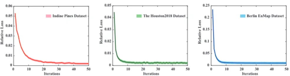
Figure 4: Convergence analysis of the proposed IMR method on three different datasets: Indine Pines, Houston2018, and Berlin EnMap. Note that the relative loss recorded in the convergence curve is obtained by averaging the loss values of multiple outer iterations in our proposed method.
sulting optimization problem can be formulated as
223 min W β 4kWZk1,1 s.t.W=W T, 1/N k Wi,j0, kWk1,1=s, (9)
whose solution has been obtained with an effective ADMM as well, as presented in
224
[66]. Please note that for those samples with labels, we construct a graph-based local
225
discriminant analysis (LDA) [39] in the place of the corresponding part in the learned
226
graphW, as shown in Fig. 2. The LDA-like graph (WL) can be expressed by 227 WL(i,j)= 1 Nk
,XiandXjare the samples belonging to thek-th class;
0 ,otherwise,
(10)
whereNkdenotes the number of samples belonging tok-th class. 228
2.3.4. Updating Pseudo-labels (Ypl) 229
Given the labels (Yl) and pseudo-labels (Y (t)
pl) of the t-thstep, and the labeled (Xl) 230
and unlabeled (Xpl) samples, we can correspondingly learn the joint graph structure 231
(W(t)) in the t-thstep from the t-thlatent feature spaces (Z(t)). The learnedW(t)can 232
then be further applied to infer the pseudo-labels of next step (Y(t+1)pl ) by LP, and then
233
the updated pseudo-labels can be fed into a next-round model learning. This process is
234
illustrated in Fig. 3. Please note that the model’s iteration will be suspended as long as
235
the to-be-learned adjacency matrixWis not changed or the residual error () between
236
the currentW(t)and the former stepW(t−1)are close to zero (e.g.,10−6). 237
2.4. Convergence Analysis and Computational Complexity 238
Considering the non-convexity of Eq. (5) when all variables are considered si- 239
multaneously, a common and effective solution for the optimization problem is using 240
a block coordinate descent (BCD) by alternatively optimizing each subproblem with 241
respect toA,S, andWin an alternating strategy. The BCD algorithm has been guar- 242
anteed in theory to converge to a stationary point, if and only if each to-be-estimated 243
variable in Eq. (5) can be exactly minimized [64]. Owing to the convexity in each 244
independent task, an unique minimum can be ideally found in our case when the La- 245
grangian parameters used in ADMM are updated within finitely iterative steps [65]. 246
The same or similar criterion has been successfully applied in various practical appli- 247
cations [10, 67, 68, 69]. In addition, we also draw the convergence curves correspond- 248
ing to the three used datasets, respectively, by recording the relative loss of objective 249
function of Eq. (5) in each iteration, as shown in Fig. (4). One can be seen from the 250
figure is that our model is able to fast reach the state of convergence with more or less 251
20 steps. 252
As observed in Section 2.3:Model Learning, the computational cost in our IMR 253
model is mainly dominated by matrix products, where the most costly step lies in solv- 254
ingS, yielding an overallO(d(2N+M)2t)computational cost for Eq. (5). 255
3. Experiments 256
3.1. Data Description 257
Three popular and promising HSI datasets – Indian Pines [70], Houston2018 [71], 258
and Berlin EnMap [72] – are used to assess the quantitative and qualitative performance 259
of the IMR method, as briefly described below. 260
3.1.1. Indian Pines Dataset 261
The hyperspectral scene located in the northwestern Indiana, USA, has been widely 262
used in various HSI-related tasks, such as dimensionality reduction [27, 56] and clas- 263
sification [73]. It consists of145×145 pixels with 220 spectral bands covering the 264
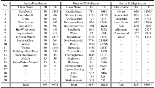
Table 1: Scene categories of the three HSI datasets used and the corresponding number of training and test samples for each class.
No. IndianPine dataset Houston2018 dataset Berlin EnMap dataset
Class Name TR TE Class Name TR TE Class Name TR TE
1 CornNotill 50 1384 HealthyGrass 711 9088 Forest 656 11075
2 CornMintill 50 784 StressedGrass 3323 29179 Residential 825 56601
3 Corn 50 184 ArtificialTurf 171 513 Industrial 446 3735
4 GrassPasture 50 447 EvergreenTrees 954 12634 Low Plants 673 12006
5 GrassTrees 50 697 DeciduousTrees 350 4698 Soil 688 3040
6 HayWindrowed 50 439 BareEarth 664 3852 Allotment 415 2427
7 SoybeanNotill 50 918 Water 82 184 Commercial 367 4938
8 SoybeanMintill 50 2418 Residential 5375 34387 Water 184 1242
9 SoybeanClean 50 564 NonResidential 7794 215890 – – – 10 Wheat 50 162 Roads 3824 41986 – – – 11 Woods 50 1244 Sidewalks 1455 32547 – – – 12 BuildingsGrassTrees 50 330 Crosswalks 148 1368 – – – 13 StoneSteelTowers 50 45 Thoroughfares 4645 41713 – – – 14 Alfalfa 15 39 Highways 271 9578 – – – 15 GrassPastureMowed 15 11 Railways 391 6546 – – – 16 Oats 15 5 PavedParking 1271 10204 – – – 17 – – – UnpavedParking 20 95 – – – 18 – – – Cars 532 6046 – – – 19 – – – Trains 154 5211 – – – 20 – – – StadiumSeats 503 6321 – – –
Total 695 9671 Total 9867 116123 Total 4254 95064
the scene that are mostly vegetation, as detailed in Table 1 along with the number of
266
training and test samples. Fig. 6 shows the false-color image of the studied scene as
267
well as the distribution of training and test samples used in [74, 56].
268
3.1.2. Houston2018 Dataset
269
This dataset is multi-modal data provided for the 2018 IEEE GRSS data fusion
270
contest, where the HSI was acquired by an ITRES CASI 1500 sensor. The HSI, with
271
dimensions of601×2384×50, was collected from the wavelengths between 380nm
272
to 1050nmat a ground sampling distance (GSD) of 1m. This is a complex city scene
273
with 20 challenging classes (see Fig. 7 and Table 1 for more details, including the
274
specific training and test information). Note that we downsampled the ground truth
275
map to the same GSD with the HSI by the nearest-neighbor-interpolation.
276
3.1.3. Berlin EnMap Dataset
277
The EnMap HSI with a GSD of 30mwas simulated by the corresponding HyMap
278
data [75] over a hybrid area that includes urban, rural, and vegetation in Berlin,
many, this data is openly and freely available from the website2. This image consists 280
of797×220pixels and 244 spectral bands in the wavelength ranging from 400nmto 281
2500nm. The ground truth in the scene is generated by the OpenStreetMap [76] in the 282
form of land cover and land use, and further refined and corrected by means of Google 283
Earth. Table 1 lists the scene categories and the number of training and test samples, 284
while the false-color image and corresponding distribution of training and test samples 285
are given in Fig. 8. 286
3.2. Experimental Configuration 287
3.2.1. Evaluation Metrics 288
With the input of different dimension-reduced features, we adopt the pixel-wise 289
classification as a potential application for quantitative evaluation in terms of classifi- 290
cation or recognition accuracy. More specifically, three commonly-used indices,Over- 291
all Accuracy (OA),Average Accuracy (AA), andKappa Coefficient (κ), are computed 292
to quantify the experimental results using two simple but effective classifiers: nearest 293
neighbor (NN) and linear SVM (LSVM). In our case, the two classifiers were selected 294
because those more powerful classifiers (e.g., kernel SVM, random forest, deep neural 295
network) tend to result in confusing evaluation, as it is unknown whether the perfor- 296
mance improvement originates from either these advanced classifiers or the features 297
itself. 298
3.2.2. Comparison with State-of-the-Art Baselines 299
We evaluate the performance of the proposed IMR model visually and quantita- 300
tively in comparison with eight state-of-the-art baselines, including 301
• Non-HDR: original spectral features (OSF); 302
• Supervised HDR: feature space discriminant analysis (FSDA) [54], joint learn- 303
ing (JL) [63]; 304
• Semi-supervised subspace learning for HDR: semi-supervised local
discrim-305
inant analysis (SELD) [60], collaborative discriminative manifold embedding
306
(CDME) [77];
307
• GLP-based semi-supervised HDR: soft-label LDA (SL-LDA) [61],
semi-super-308
vised fisher local discriminant analysis (SSFLDA) [62].
309
3.2.3. Implementation Preparation
310
The parameter settings for the algorithms play a key role in performance
assess-311
ment. A common tactic for model selection is to run cross-validation on the
train-312
ing set. Following that, we conducted a 10-fold cross-validation to determine the
313
optimal parameter combination for the different algorithms. In detail, there
param-314
eters that need to be tuned to maximize the classification performance on the
train-315
ing set were subspace dimension3 (d
sub), selected from5to50at intervals of5; the 316
number of nearest neighbors (k); the standard deviation (σ) in SELD and SSLFDA,
317
ranging from{10,20, ...,50} and{10−2,10−1,100,101,102}, respectively; and the 318
regularization parameters (e.g., α and β) in JL, CDME, and IMR in the range of
319
{10−2,10−1,100,101,102}, while another regularization parameterγin IMR can be 320
selected from{0.1,0.2, . . . ,0.9}. Moreover, initializing the adjacency matrix (W) and
321
pseudo-labels (Ypl) in IMR is also an important factor in determining the model’s per-322
formance. We first predict the unlabeled samples using a pre-trained classifier on the
323
training set; then the predicted results can be naturally input into the model as
pseudo-324
labels. Likewise, the initializedWcan be given by the labels and pseudo-labels. In
325
addition, note that the clustering technique (e.g., K-means) is applied to handle the
326
highly computational complexity caused by the large quantity of unlabeled samples
327
during the process of model learning. As a trade-off, the number of cluster centers
328
used in our case is approximately set to be the same as that of the training samples.
329
3For LDA-based approaches, e.g., FSDA, SELD, SL-LDA, and SSLFDA, the class number minus 1 is
iterative 0 iterative 1 iterative 2 iterative 3 iterative 4 78.13% 81.36% 82.51% 82.80% 82.14% 72.19% 75.09% 75.67% 76.04% 76.26% 10 11 12 13 14 15 16 1 2 3 4 5 6 7 8 9 10 11 12 13 14 15 16 10 11 12 13 14 15 16 10 11 12 13 14 15 16 10 11 12 13 14 15 16 NN classifier LSVM classifier
(a) Indian Pines dataset
iterative 0 iterative 1 iterative 2 iterative 3 iterative 4 64.85% 69.67% 70.37% 71.55% 71.11% 65.03% 67.15% 67.81% 68.37% 67.95% 10 11 12 13 14 15 16 17 18 19 20 1 2 3 4 5 6 7 8 9 10 11 12 13 14 15 16 17 18 19 20 10 11 12 13 14 15 16 17 18 19 20 10 11 12 13 14 15 16 17 18 19 20 10 11 12 13 14 15 16 17 18 19 20 NN classifier LSVM classifier (b) Houston2018 dataset
iterative 0 iterative 1 iterative 2 iterative 3 iterative 4
62.98% 64.35% 66.83% 67.39% 68.24% 69.56% 71.13% 74.11% 75.03% 73.51% 1 2 3 4 5 6 7 8 NN classifier LSVM classifier
(c) Berlin EnMap dataset
Figure 5: Visual and quantitative (OA) performance analysis with the different number of iterations in IMR on the three datasets.
3.2.4. The Number of Iterations in the Proposed IMR 330
According to the model’s stopping criteria inAlgorithm 1, our IMR method gen- 331
Training
OSF FSDA JL SELD CDME SL-LDA SSLFDA IMR-3
FalseColor
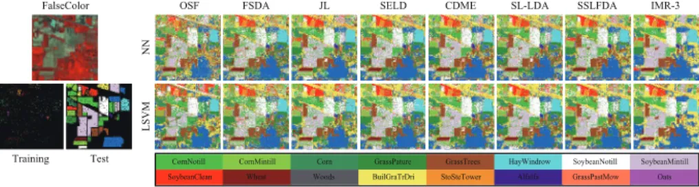
CornNotill CornMintill Corn GrassPature GrassTrees HayWindrow SoybeanNotill SoybeanMintill SoybeanClean Wheat Woods BuilGraTrDri StoSteTower Alfalfa GrassPastMow Oats Test N N L S V M
Figure 6: False-color image, the distribution of training and test samples as well as classification maps of the compared methods using two different classifiers on the Indian Pines dataset.
matrix (W) out of three or four iterations. To support the results more effectively, we
333
further investigate the effects of assigning a different number of iterations in IMR for
334
the three datasets. Fig. 5 gives both visual and quantitative results with the increase
335
of the IMR’s iterations4. Note that the IMR withiterative 0equivalently degrades to a 336
version without label propagation. The OAs are clearly much lower without using an
it-337
erative strategy to update pseudo labels (iterative 0) than when using several iterations.
338
Intuitively, this proves the superiority of the iterative strategy by gradually optimizing
339
the pseudo-labels. It is worth noting, however, that the performance gain starts to slow
340
down after two iterations and then remains essentially stable in the follow-up iterations,
341
as the variableWis hardly changed any further. Similarly, for the different number of
342
iterations, there is a consistent trend in the compactability of intra-class and the
separa-343
bility of inter-class. To summarize, we determine the number of iterations in the IMR
344
to be 3 (IMR-3 for short); it will be used for comparison in the following experiments.
345
3.3. Results and Analysis
346
3.3.1. The Indian Pines Dataset
347
Fig. 6 presents the classification maps for different HDR compared methods using
348
two classifiers on the Indian Pines dataset; Table 2 correspondingly lists the quantitative
349
results obtained under the optimal parameter combination.
350
Using the NN classifier, there is basically the same classification performance in
351
OSF and FSDA. Despite an improved supervised criteria, FSDA still yields poor
clas-352
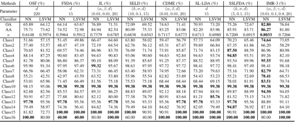
Table 2: Quantitative performance comparison among the different algorithms with the optimal parameters
on the IndianPines dataset in terms of OA, AA, andκas well as accuracy for each class. The best is shown
in bold. Note that IMR-3 denotes the IMR with three iterations.
Methods OSF (%) FSDA (%) JL (%) SELD (%) CDME (%) SL-LDA (%) SSLFDA (%) IMR-3 (%) Parameter d d (α, β, d) (k, σ, d) (α, β, d) d (k, σ, d) (α, β, γ, d) 220 15 (0.01,0.01,20) (10,0.1,15) (0.01,0.01,20) 15 (5,0.1,15) (0.01,0.1,0.8,20) Classifier NN LSVM NN LSVM NN LSVM NN LSVM NN LSVM NN LSVM NN LSVM NN LSVM OA 65.89 64.12 64.14 63.67 76.89 71.51 72.09 69.52 74.63 71.41 70.93 73.20 75.26 72.67 82.80 76.04 AA 75.71 73.62 74.52 72.98 84.94 82.54 80.09 75.33 83.25 83.06 82.20 83.96 85.91 83.71 86.27 81.80 κ 0.6148 0.5974 0.5964 0.5912 0.7379 0.6785 0.6838 0.6543 0.7117 0.6773 0.6713 0.6980 0.7200 0.6915 0.8033 0.7266 Class1 51.66 57.15 51.45 49.86 66.47 64.60 63.80 58.02 59.47 56.79 57.73 64.09 70.23 65.46 74.64 73.05 Class2 57.40 53.57 48.47 47.19 72.19 64.54 62.76 56.12 65.31 67.47 59.69 66.84 67.35 61.86 66.20 58.29 Class3 70.65 81.52 69.57 74.46 86.96 83.70 76.09 71.74 73.91 85.87 71.74 83.15 87.50 88.59 86.96 80.98 Class4 88.14 87.25 90.60 83.45 94.63 90.83 93.06 90.60 94.63 92.84 94.63 93.74 94.85 93.51 89.26 82.10 Class5 81.78 80.06 86.80 86.37 90.10 88.09 91.39 85.65 91.25 87.37 88.52 88.95 93.54 89.96 95.55 91.68 Class6 95.90 91.34 97.95 97.49 99.32 95.67 98.63 97.95 97.72 97.72 98.41 97.72 98.41 97.49 98.41 98.18 Class7 66.56 66.45 58.06 62.31 73.31 66.45 63.40 58.93 74.95 72.66 73.20 79.63 75.16 71.90 82.79 64.71 Class8 55.21 42.51 42.97 43.59 63.52 53.80 55.96 55.54 62.82 53.89 54.43 53.23 55.21 52.69 78.41 68.53 Class9 53.01 65.96 71.45 66.49 81.56 75.18 75.53 75.18 68.44 68.44 68.44 69.15 78.01 81.91 83.51 70.74 Class10 98.15 95.06 99.38 99.38 99.38 99.38 99.38 99.38 99.38 99.38 99.38 99.38 99.38 99.38 99.38 99.38 Class11 82.88 82.56 85.53 84.57 89.31 86.25 88.83 89.07 92.12 88.18 87.94 88.91 89.87 88.99 94.50 94.05 Class12 50.91 67.27 77.88 80.61 82.12 80.00 77.58 78.79 80.91 83.64 81.21 85.76 81.52 75.15 74.55 71.82 Class13 97.78 95.56 97.78 95.56 95.56 97.78 95.56 93.33 95.56 97.78 97.78 93.33 97.78 95.56 88.89 91.11 Class14 79.49 58.97 74.36 56.41 84.62 74.36 79.49 64.10 84.62 76.92 82.05 79.49 94.87 76.92 87.18 64.10 Class15 81.82 72.73 100.00 100.00 100.00 100.00 100.00 90.91 90.91 100.00 100.00 100.00 90.91 100.00 100.00 100.00 Class16 100.00 80.00 40.00 40.00 80.00 100.00 60.00 40.00 100.00 100.00 100.00 100.00 100.00 100.00 80.00 100.00
sification accuracy, since directly projecting the original data into a discriminative sub- 353
space with the limited amount of labeled samples is very challenging, especially when 354
dealing with noisy data (e.g., HSI) with various spectral variabilities. Overall, the clas- 355
sification performance by considering the unlabeled samples is better than that without 356
considering them. It should be noted, however, that inspired by latent subspace learn- 357
ing, the JL model dramatically outperforms FSDA (more than 10%improvement), but 358
also improves the OAs of around 4%, 6%, 2%, and 1%, respectively, compared to those 359
semi-supervised HDR approaches (SELD, CDME, SL-LDA, and SSLFDA). This intu- 360
itively indicates the superiority of the regression-based JL model for feature learning. 361
Following the JL-like model, the proposed IMR framework achieves the best perfor- 362
mance owing to the multitask learning framework, where the labeled and unlabeled 363
samples can be jointly regressed, and to the iterative updating strategy of pseudo-labels. 364
There is a similar trend in classification performance using the LSVM classifier, yet its 365
performance is relatively weaker than those with the NN classifier. The possible reason 366
for that is the few training samples available, further leading to the poor estimation of 367
decision boundary for the SVM-like classifier learning. 368
Furthermore, we can observe from Table 2 that our IMR not only outperforms 369
other HDR methods in terms ofOA,AA, andκ, but it also obtains highly competitive 370
results for each class, particularly for those classes with a relatively limited number 371
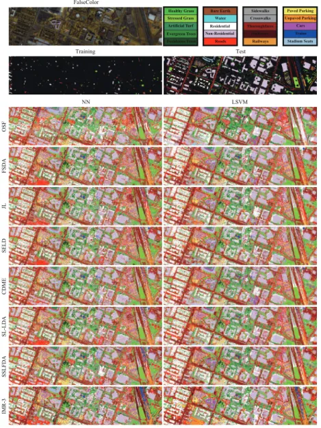
Healthy Grass Stressed Grass Artificial Turf Evergreen Trees Deciduous Trees Bare Earth Water Residential Non-Residential Roads Sidewalks Crosswalks Thoroughfares Highways Railways Paved Parking Unpaved Parking Cars Trains Stadium Seats O S F F S D A JL S E L D CD M E S L -L D A S S L F D A NN LSVM IM R-3 FalseColor Training Test
Figure 7: False-color image, the distribution of training and test samples as well as classification maps of compared methods using two different classifiers on the Houston2018 dataset.
Notill,Grass-Trees,Soybean-Notill,Soybean-Mintill,Soybean-Clean, andWheat. This
373
provides powerful evidence of the effectiveness of transferring the unlabeled samples
374
to the learned subspace and the superiority of iteratively optimizing pseudo-labels.
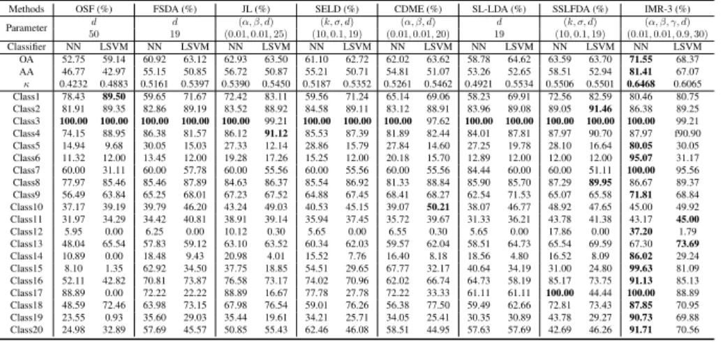
Table 3: Quantitative performance comparison among the different algorithms with the optimal parameters
on the Houston2018 dataset in terms of OA, AA, andκas well as accuracy for each class. The best is shown
in bold. Note that IMR-3 denotes the IMR with three iterations.
Methods OSF (%) FSDA (%) JL (%) SELD (%) CDME (%) SL-LDA (%) SSLFDA (%) IMR-3 (%) Parameter 50d 19d (0.01(α, β, d,0.01,)25) (10(k, σ, d,0.1,19)) (0.01(α, β, d,0.01,)20) 19d (10(k, σ, d,0.1,19)) (0.01(α, β, γ, d,0.01,0.9),30) Classifier NN LSVM NN LSVM NN LSVM NN LSVM NN LSVM NN LSVM NN LSVM NN LSVM OA 52.75 59.14 60.92 63.12 62.93 63.50 61.10 62.72 62.02 63.62 58.78 64.62 63.59 63.70 71.55 68.37 AA 46.77 42.97 55.15 50.85 56.72 50.87 55.21 50.71 54.81 51.07 53.26 52.65 58.51 52.94 81.41 67.07 κ 0.4232 0.4883 0.5161 0.5397 0.5390 0.5450 0.5187 0.5352 0.5261 0.5462 0.4921 0.5534 0.5506 0.5501 0.6468 0.6065 Class1 78.43 89.50 59.65 71.67 72.42 83.11 59.56 71.24 65.14 69.06 58.23 69.91 72.56 82.59 80.46 80.75 Class2 81.91 89.35 82.86 89.19 83.52 88.92 84.58 89.11 83.12 88.91 83.96 89.08 89.05 91.46 86.38 89.25 Class3 100.00 100.00 100.00 100.00 100.00 99.21 100.00 100.00 100.00 97.62 100.00 100.00 100.00 100.00 100.00 99.21 Class4 74.15 88.95 86.38 81.57 86.12 91.12 85.53 87.39 81.89 82.44 84.01 87.81 87.97 90.70 87.97 f90.90 Class5 14.94 9.68 30.05 15.03 27.33 12.14 28.86 15.79 27.84 14.60 27.25 19.78 28.10 16.64 80.05 30.05 Class6 11.32 12.00 13.45 12.00 19.28 17.26 15.25 12.00 20.18 15.70 12.89 12.00 12.00 12.00 95.07 31.17 Class7 60.00 31.11 60.00 57.78 60.00 55.56 60.00 55.56 60.00 55.56 84.44 60.00 60.00 51.11 100.00 95.56 Class8 77.97 85.46 85.46 87.89 84.63 86.37 85.54 86.92 81.33 88.84 85.90 85.70 87.29 89.95 86.67 89.37 Class9 56.49 63.84 65.25 68.01 67.23 67.52 64.88 67.45 68.41 68.27 62.54 71.53 65.07 65.58 71.81 68.84 Class10 37.17 39.19 39.79 46.20 43.24 49.03 40.53 45.15 39.07 50.21 38.07 46.77 48.92 47.65 45.00 49.92 Class11 31.97 34.29 34.42 40.81 38.91 39.14 35.94 37.45 35.72 39.67 31.33 36.21 43.78 41.38 43.17 45.00 Class12 5.95 0.00 6.25 0.00 10.12 0.30 5.65 0.00 6.55 0.30 5.65 0.00 17.86 0.00 37.20 1.79 Class13 48.04 65.54 57.83 59.12 63.10 63.52 60.34 62.03 59.57 62.04 58.51 64.73 65.54 69.59 67.30 73.69 Class14 10.89 0.00 18.48 9.43 20.98 4.01 15.52 7.76 16.40 8.18 18.56 4.80 16.52 8.09 86.02 29.24 Class15 8.10 1.35 62.92 34.50 37.75 18.85 54.51 29.65 67.77 32.17 40.64 34.19 31.00 24.80 99.63 81.09 Class16 52.11 42.82 70.81 73.87 76.58 73.17 74.02 70.96 62.02 66.74 64.73 58.19 85.17 73.75 91.13 85.13 Class17 88.89 0.00 72.22 22.22 88.89 16.67 77.78 27.78 72.22 33.33 61.11 61.11 100.00 44.44 100.00 88.89 Class18 48.59 72.46 63.98 73.15 67.98 76.54 59.01 76.26 56.38 77.50 59.49 62.66 72.81 73.43 87.85 70.95 Class19 23.55 0.93 35.60 29.03 35.44 19.61 34.21 25.71 34.05 25.41 30.35 30.89 43.78 29.27 90.73 69.88 Class20 24.98 32.89 57.69 45.57 50.85 55.43 62.46 46.08 58.51 44.95 57.63 57.69 42.69 46.26 91.71 70.56
3.3.2. The Houston2018 Dataset 376
Classification performance using the different low-dimensional feature represen- 377
tations is evaluated on the Houston2018 dataset both visually and quantitatively, as 378
shown in Fig. 7 and listed in Table 3, respectively. The optimal parameters used for 379
different compared methods are given in Table 3 as well. Likewise, due to more chal- 380
lenging categories in this scene and small-scale training set, the ability to classify the 381
materials for the LSVM is limited. This might explain a phenomena in Table 3, that is, 382
why the NN-based classifier, to some extent, performs better than the SVM-based one 383
for many compared methods. 384
More specifically, OSF yields a poor classification performance, due to the highly 385
redundant spectral information and the sensitivity to noise. Unlike OSF that directly 386
uses the original spectral features as the input features, FSDA and JL are apt to discrim- 387
inate the materials due to the utilization of the label information. Further, taking the 388
unlabeled samples into account is of great benefit in finding a better decision bound- 389
ary, yielding a possible performance improvement, as shown in those subspace-based 390
learning semi-supervised HDR methods (e.g., SELD, CDME). It is worth noting that 391
the regression-based JL model is provided with nearly identical performance to those 392
Table 4: Quantitative performance comparison among the different algorithms with the optimal parameters
on the Berlin EnMap dataset in terms of OA, AA, andκas well as accuracy for each class. The best is shown
in bold. Note that IMR-3 denotes the IMR with three iterations.
Methods OSF (%) FSDA (%) JL (%) SELD (%) CDME (%) SL-LDA (%) SSLFDA (%) IMR-3 (%) Parameter d d (α, β, d) (k, σ, d) (α, β, d) d (k, σ, d) (α, β, γ, d) 244 7 (0.01,0.1,20) (10,0.1,7) (0.01,0.01,15) 7 (25,0.1,7) (0.1,0.01,0.8,20) Classifier NN LSVM NN LSVM NN LSVM NN LSVM NN LSVM NN LSVM NN LSVM NN LSVM OA 53.97 67.87 61.51 67.77 62.56 68.47 61.55 69.86 60.88 69.05 60.53 66.01 60.87 70.13 67.39 75.03 AA 57.47 66.04 64.61 65.98 64.71 65.90 63.79 65.76 62.88 65.13 63.87 65.34 65.96 67.36 69.05 69.36 κ 0.3781 0.5372 0.4711 0.5299 0.4821 0.5392 0.4702 0.5540 0.4621 0.5469 0.4619 0.5142 0.4668 0.5620 0.5411 0.6222 Class1 61.82 79.41 76.14 74.43 78.50 76.25 75.54 78.57 73.35 80.55 78.61 80.15 74.18 80.26 80.48 81.91 Class2 51.39 67.42 57.50 68.11 58.89 68.94 57.70 70.92 57.80 69.92 55.75 64.37 55.92 70.32 64.81 77.61 Class3 43.72 55.56 55.26 56.79 56.79 57.40 51.35 54.00 49.16 58.31 49.02 53.47 51.94 53.65 61.95 61.85 Class4 60.06 70.63 70.66 69.71 70.40 70.66 72.62 71.78 71.16 71.02 72.51 72.83 71.71 72.91 74.76 73.60 Class5 89.54 87.63 89.90 91.68 90.46 92.43 90.89 92.47 92.11 92.96 90.69 93.36 92.83 90.59 91.87 88.82 Class6 59.21 66.50 61.93 65.55 61.48 64.40 58.71 60.77 61.35 62.22 60.53 64.81 67.33 64.94 68.44 65.06 Class7 32.46 40.06 38.01 40.54 37.04 38.29 37.26 38.80 30.96 28.03 33.29 30.34 42.89 42.45 36.55 42.79 Class8 61.51 61.11 67.47 61.03 64.09 58.78 66.26 58.78 67.15 58.05 70.53 63.37 70.85 63.77 73.51 63.29
the powerful GLP is utilized (e.g., SL-LDA, SSLFDA). As expected, the performance
394
of the IMR framework, which optimizes the pseudo-labels in an iterative fashion, is
395
dramatically superior to that of others with the OA’s increase of approximately 8%
396
(NN) and 5%(LSVM).
397
More intuitively, the proposed IMR performs better at identifying each material
398
than other methods. In particular, when facing the extremely unbalanced sample
distri-399
bution (see Table 1), our method gradually improves the quality of the pseudo-labels,
400
thereby making the model develop a more powerful learning ability. Table 3 also
re-401
veals an interesting but unsurprising result: for those classes with a very limited number
402
of training samples (e.g.,Deciduous Trees,Bare Earth,Water,Crosswalks,Highways,
403
Unpaved Parking, andStadium Seats), the IMR makes a significant performance gain
404
(an increase of at least 50% for these classes) with the aid of iterative pseudo-label
405
learning.
406
3.3.3. The Berlin EnMap Dataset
407
For the Berlin EnMap dataset, the visual comparison of eight different algorithms
408
in the form of classification maps is shown in Fig. 8. Table 4 details the comparison by
409
means of three quantitative indices:OA,AA, andκ.
410
With a very high spectral dimension (244), OSF only holds a 53.97% accuracy
411
when using the NN classifier. The performance of supervised HDR methods (SFDA
412
and JL) is obviously superior to that of OSF, with an increase of at least 8% using
413
the NN classifier. This reveals the importance of HDR in the follow-up
Forest Residential Industrial Low Plants Soil Allotment Commercial Water Unlabeled FalseColor Training Test NN LSVM O S F F S D A JL S E L D C D M E S L -L D A S S L F D A IM R -3
Figure 8: False-color image, the distribution of training and test samples as well as classification maps of compared methods using two different classifiers on the EnMap Berlin dataset.
LSVM classifier, where JL shows a better classification performance owing to its
well-416
designed architecture in the regression-based latent subspace learning. SELD learns the
417
subspace projections by not only considering the label information but also computing
418
the similarities between the unlabeled samples, yielding an effective semi-supervised
419
low-dimensional embedding. However, the similarities between samples are usually
420
measured by certain fixed functions, i.e., radial basis function (RBF), in the
high-421
dimensional space, leading to poor robustness and ability to generalize. CDME
imple-422
ments an automatic similarity measurement by collaboratively representing the
con-423
nectivity between the samples for the low-dimensional embedding. By the means of
424
the soft (or pseudo) labels instead of using similarity measurement, SL-LDA and
SS-425
FLDA jointly use the labels and pseudo-labels to find a high discriminative subspace
426
in a semi-supervised embedding approach.
427
Beyond the two subspace-based (SELD and CDME) and two GLP-based
(SL-428
LDA and SSFLDA) semi-supervised strategies, we propose to iteratively optimize the
429
pseudo-labels and feed them into a multitask regression framework in order to find a
430
latent optimal subspace where the final decision boundary for different classes can be
431
easily determined. On the other hand, our proposed IMR for each of the classes in
432
the studied image exceeds the vast majority of compared methods except the material
433
of Commercial, thereby further revealing the IMR’s advantages in low-dimensional
434
representation learning.
435
3.4. Parameter Sensitivity Analysis
436
3.4.1. On the Regularization Parameters
437
The quality of low-dimensional features extracted by the proposed IMR model is,
438
to some extent, sensitive to the selection of three regularization parameters (α,β, and
439
γ) as shown in Eq. (5). For this reason, we experimentally investigate the effects of
440
different parameter setting in terms of OA via the NN classifier. The resulting analysis
441
on the three datasets is quantified in Fig. 9, where the parameter combinations of(γ=
442
0.8, α= 0.01, β = 0.1),(γ= 0.9, α= 0.01, β= 0.01), and(γ = 0.8, α= 0.1, β =
443
0.01)obtain the optimal classification performance on the test set for the Indine Pines
10-4 10-3 10-2 10-1 10 0 101 102 α 60 65 70 75 80 85 O A (%) Indine Pines Houston2018 Berlin EnMap β 55 60 65 70 75 80 85 O A (%) 10-4 10-3 10-2 10-1 10 0 101 102 Indine Pines Houston2018 Berlin EnMap 0.1 0.2 0.3 0.4 0.5 0.6 0.7 0.8 0.9 1.0 γ 55 60 65 70 75 80 85 O A (%) Indine Pines Houston2018 Berlin EnMap
Figure 9: Sensitivity analysis on the regularization parameters (e.g.,α,β, andγ) of the IMR in Eq. (5).
Subspace Dimension 55 60 65 70 75 80 85 O A (%) Indine Pines 5 10 15 20 25 30 35 40 45 50 Subspace Dimension 62 64 66 68 70 72 74 Houston2018 O A (%) 5 10 15 20 25 30 35 40 45 50 Subspace Dimension 60 62 64 66 68 70 Berlin EnMap O A (%) 5 10 15 20 25 30 35 40 45 50
Figure 10: Sensitivity analysis on the subspace dimension in the proposed IMR method.
regrading the parameter setting are basically consistent with those obtained by cross- 446
validation on the training set (see the Section 3.2.3: Implementation Preparation). 447
Thus, the cross-validation strategy can be effectively used to determine the model’s 448
parameters so that other researchers can produce the results for their tasks. 449
3.4.2. On the Subspace Dimension 450
Apart from the regularization parameters, we analyze the performance gain in us- 451
ing the different subspace dimension of our IMR method, since a proper subspace 452
dimension tends to reach a trade-off between discrimination and redundancy of the 453
dimension-reduced product. For this purpose, the corresponding experiments are con- 454
ducted by using the NN classifier to see the classification performance with the gradually- 455
reducing dimension. As can be seen from Fig. 10, with the increase of subspace di- 456
mension, the IMR’s performance sharply increases to around 20 for first dataset, 30 for 457
the second dataset, and 20 for the last dataset, respectively, then starts to reach a rel- 458
atively stable state, and finally decreases with a slight perturbation when the subspace 459
5% 10% 15% 20% 25% 30% 35% 40% 45% 50% Training Rate 60 70 80 90 100 O A (%) NN LSVM 5% 10% 15% 20% 25% 30% 35% 40% 45% 50% Training Rate 60 65 70 75 80 85 O A (%) NN LSVM 5% 10% 15% 20% 25% 30% 35% 40% 45% 50% Training Rate 60 65 70 75 80 85 90 95 NN LSVM O A (%)
Indine Pines Dataset Houston2018 Dataset Berlin EnMap Dataset
Figure 11: Sensitivity analysis to the size of training set using the NN and LVSM classifiers for the used three datasets.
3.4.3. On the Training Set Size
461
Although the IMR adopts the semi-supervised learning strategy by jointly
account-462
ing for the labeled and unlabeled samples, yet the HDR’s performance is determined
463
by the number of training samples to a great extent. This is, therefore, indispensable to
464
investigate the sensitivity with an increasing size of training set. To highlight and
em-465
phasize the effectiveness and superiority of our proposed method in the HDR issue, we
466
arrange the classification task by resetting the training set randomly selected from all
467
labeled samples out of 10 run with the different proportions in the range of 5% to 50%
468
at a 5% interval and the rest as the test set, and the average classification accuracies are
469
reported by integrating the ten outputs in the end. Fig. 11 shows a similar trend in OAs
470
with two classifiers (NN and LSVM) on the three different datasets, that is, the
clas-471
sification performance improves with the size of training set, faster in the early, and
472
later basically stabilized. This also indicates that our semi-supervised method is not
473
heavily dependent on a large-scale training set, which can hold a desirable and
com-474
petitive performance in HDR, even when only small-scale labeled samples are used
475
for training. On the other hand, we can observe an interesting conclusion on the first
476
two datasets from the Fig. 11 that the NN classifier outperforms the LSVM one when
477
the training samples are insufficient, e.g., less than around 15% of total samples. This
478
could be well explained by the fact that LSVM is a learning-based classifier depending
479
on the adequate samples for training an effective model, which is also supported by the
480
experimental results yielding the higher OAs using the LSVM than those using the NN
481
while using more training samples. Furthermore, with the increasing of training
sam-482
Table 5: Time cost for the HDR of different methods on the three datasets.
Datasets Time Cost (s)
OSF FSDA JL SELD CDME SL-LDA SSFLDA IMR
Indine Pines – 0.06 4.60 9.68 1.85 2.32 3.13 51.05
Houston2018 – 0.09 41.25 192.22 12.06 12.77 24.88 132.41
Berlin EnMap – 0.22 48.81 57.81 10.82 11.48 25.20 75.72
probably due to the lack of the spatial information modeling. 484
3.5. Computational Cost in Different Methods 485
The experiments for HDR conducted by different methods are implemented for 486
simulation on a laptop with the CPU i7-6700HQ (2.60GHz) and a 32GB random access 487
memory (RAM). Herein, we assess the operational efficiency of the compared HDR 488
approaches in terms of running time, as listed in Table 5. 489
In general, the running time of supervised HDR is much less than that of semi- 490
supervised HDR, such as between supervised discriminant analysis (FSDA) and semi- 491
supervised discriminant analysis (SELD, CDME, SL-LDA, and SSFLDA). The conclu- 492
sion is just as much applicable to another group, that is, JL and our proposed IMR. Re- 493
markably, although the newly-proposed IMR model seems to be operationally complex 494
compared to other HDR methods, yet as it turns out, the IMR shows the computation- 495
ally efficiency and the time cost is acceptable, mainly owing to the fast matrix-based 496
computing power in regression-based techniques. 497
4. Conclusions 498
To facilitate the use of unlabeled samples effectively and efficiently, we propose a 499
novel regression-based semi-supervised HDR model, called iterative multitask regres- 500
sion (IMR), which 1) simultaneously bridges the labeled and unlabeled samples with 501
the labels and pseudo-labels in a multitask regression framework; and 2) progressively 502
updates the pseudo-labels in an iterative fashion. This model provides us a new insight 503
into the solutions of HDR-related problems. We conducted extensive experiments on 504
three convincing and challenging HSI datasets, demonstrating that our method (IMR) 505
is capable of extracting more discriminative features by allowing for the unlabeled 506
It should be noted, however, that while there has been a desirable performance boost
508
in IMR, it is still limited to working well only by linearly learning the low-dimensional
509
feature representations for complex nonlinear cases. For this reason, our future work
510
will address the HDR issue in a more complex scene and extend our framework to a
511
nonlinear one with possible spatial information modeling.
512
5. Acknowledgements 513
The authors would like to thank the Hyperspectral Image Analysis group and the
514
NSF Funded Center for Airborne Laser Mapping (NCALM) at the University of
Hous-515
ton for providing the CASI University of Houston dataset.
516
This work was supported by funding from the European Research Council (ERC)
517
under the European Union’s Horizon 2020 research and innovation program (grant
518
agreement No [ERC-2016-StG-714087]) and from Helmholtz Association under the
519
framework of the Young Investigators Group ”SiPEO” (VH-NG-1018, www.sipeo.bgu.
520
tum.de). The work of N. Yokoya was supported by Japan Society for the Promotion of
521
Science (JSPS) KAKENHI 15K20955.
522
[1] A. Plaza, J. A. Benediktsson, J. W. Boardman, J. Brazile, L. Bruzzone, G.
Camps-523
Valls, J. Chanussot, M. Fauvel, P. Gamba, A. Gualtieri, et al., Recent advances in
524
techniques for hyperspectral image processing, Remote sensing of environment
525
113 (2009) S110–S122.
526
[2] H. Yu, L. Gao, W. Liao, B. Zhang, A. Piˇzurica, W. Philips, Multiscale
superpixel-527
level subspace-based support vector machines for hyperspectral image
classifica-528
tion, IEEE Geoscience and Remote Sensing Letters 14 (11) (2017) 2142–2146.
529
[3] L. Gan, J. Xia, P. Du, J. Chanussot, Class-oriented weighted kernel sparse
repre-530
sentation with region-level kernel for hyperspectral imagery classification, IEEE
531
Journal of Selected Topics in Applied Earth Observations and Remote Sensing
532
11 (4) (2018) 1118–1130.
533
[4] R. Hang, Q. Liu, D. Hong, P. Ghamisi, Cascaded recurrent neural networks for
hyperspectral image classification, IEEE Transactions on Geoscience and Remote 535
Sensing 57 (8) (2019) 5384–5394. 536
[5] F. Dell’Acqua, P. Gamba, A. Ferrari, J. A. Palmason, J. A. Benediktsson, 537
K. ´Arnason, Exploiting spectral and spatial information in hyperspectral urban 538
data with high resolution, IEEE Geoscience and Remote Sensing Letters 1 (4) 539
(2004) 322–326. 540
[6] C. Yang, J. H. Everitt, Q. Du, B. Luo, J. Chanussot, Using high-resolution air- 541
borne and satellite imagery to assess crop growth and yield variability for preci- 542
sion agriculture, Proc. IEEE 101 (3) (2013) 582–592. 543
[7] F. Fan, W. Fan, Q. Weng, Improving urban impervious surface mapping by linear 544
spectral mixture analysis and using spectral indices, Canadian Journal of Remote 545
Sensing 41 (6) (2015) 577–586. 546
[8] Y. Xie, Q. Weng, Spatiotemporally enhancing time-series dmsp/ols nighttime 547
light imagery for assessing large-scale urban dynamics, ISPRS Journal of Pho- 548
togrammetry and Remote Sensing 128 (2017) 1–15. 549
[9] S. Henrot, J. Chanussot, C. Jutten, Dynamical spectral unmixing of multitempo- 550
ral hyperspectral images, IEEE Transactions on Image Processing 25 (7) (2016) 551
3219–3232. 552
[10] D. Hong, N. Yokoya, J. Chanussot, X. X. Zhu, Learning low-coherence dictio- 553
nary to address spectral variability for hyperspectral unmixing, in: Proceedings 554
of IEEE International Conference on Image Processing (ICIP), 2017, pp. 1–5. 555
[11] Y. Zhong, X. Wang, L. Zhao, R. Feng, L. Zhang, Y. Xu, Blind spectral unmixing 556
based on sparse component analysis for hyperspectral remote sensing imagery, 557
ISPRS Journal of Photogrammetry and Remote Sensing 119 (2016) 49–63. 558
[12] D. Hong, N. Yokoya, J. Chanussot, X. X. Zhu, An augmented linear mixing model 559
to address spectral variability for hyperspectral unmixing, IEEE Transactions on 560
[13] C. McCann, K. S. Repasky, R. Lawrence, S. Powell, Multi-temporal mesoscale
562
hyperspectral data of mixed agricultural and grassland regions for anomaly
de-563
tection, ISPRS Journal of Photogrammetry and Remote Sensing 131 (2017) 121–
564
133.
565
[14] X. Wu, D. Hong, P. Ghamisi, W. Li, R. Tao, MsRi-CCF: Multi-scale and
rotation-566
insensitive convolutional channel features for geospatial object detection, Remote
567
Sensing 10 (12) (2018) 1990.
568
[15] C. Li, L. Gao, Y. Wu, B. Zhang, J. Plaza, A. Plaza, A real-time unsupervised
569
background extraction-based target detection method for hyperspectral imagery,
570
Journal of Real-Time Image Processing 15 (3) (2018) 597–615.
571
[16] X. Wu, D. Hong, J. Tian, J. Chanussot, W. Li, R. Tao, ORSIm Detector: A
572
novel object detection framework in optical remote sensing imagery using
spatial-573
frequency channel features, IEEE Transactions on Geoscience and Remote
Sens-574
ing 57 (7) (2019) 5146–5158.
575
[17] D. Tuia, D. Marcos, G. Camps-Valls, Multi-temporal and multi-source remote
576
sensing image classification by nonlinear relative normalization, ISPRS Journal
577
of Photogrammetry and Remote Sensing 120 (2016) 1–12.
578
[18] N. Yokoya, P. Ghamisi, J. Xia, S. Sukhanov, R. Heremans, I. Tankoyeu, B.
Bech-579
tel, B. Le Saux, G. Moser, D. Tuia, Open data for global multimodal land use
580
classification: Outcome of the 2017 ieee grss data fusion contest, IEEE Journal
581
of Selected Topics in Applied Earth Observations and Remote Sensing 11 (5)
582
(2018) 1363–1377.
583
[19] X. Zhu, Y. Hou, Q. Weng, L. Chen, Integrating uav optical imagery and lidar data
584
for assessing the spatial relationship between mangrove and inundation across
585
a subtropical estuarine wetland, ISPRS Journal of Photogrammetry and Remote
586
Sensing 149 (2019) 146–156.
587
[20] X. Liu, C. Deng, J. Chanussot, D. Hong, B. Zhao, Stfnet: A two-stream