CEC Theses and Dissertations College of Engineering and Computing
2018
The Impact of Cost on Feature Selection for
Classifiers
Richard Clyde McCrae
Nova Southeastern University,[email protected]
This document is a product of extensive research conducted at the Nova Southeastern UniversityCollege of Engineering and Computing. For more information on research and degree programs at the NSU College of Engineering and Computing, please clickhere.
Follow this and additional works at:https://nsuworks.nova.edu/gscis_etd Part of theArtificial Intelligence and Robotics Commons
Share Feedback About This Item
This Dissertation is brought to you by the College of Engineering and Computing at NSUWorks. It has been accepted for inclusion in CEC Theses and Dissertations by an authorized administrator of NSUWorks. For more information, please [email protected].
NSUWorks Citation
Richard Clyde McCrae. 2018.The Impact of Cost on Feature Selection for Classifiers.Doctoral dissertation. Nova Southeastern University. Retrieved from NSUWorks, College of Engineering and Computing. (1057)
The Impact of Cost on Feature Selection for Classifiers
by
Richard McCrae, RM1718
A dissertation report submitted in partial fulfillment of the requirements for the degree of Doctor of Philosophy
in
Computer Science
College of Engineering and Computing Nova Southeastern University
ABSTRACT
An Abstract of a Dissertation Report Submitted to Nova Southeastern University in Partial Fulfillment of the Requirements for the Degree of Doctor of PhilosophyThe Impact of Cost on Feature Selection for Classifiers by
Richard C. McCrae 2018
Supervised machine learning models are increasingly being used for medical diagnosis. The diagnostic problem is formulated as a binary classification task in which trained classifiers make predictions based on a set of input features. In diagnosis, these features are typically procedures or tests with associated costs. The cost of applying a trained classifier for diagnosis may be estimated as the total cost of obtaining values for the features that serve as inputs for the classifier. Obtaining classifiers based on a low cost set of input features with acceptable
classification accuracy is of interest to practitioners and researchers. What makes this problem even more challenging is that costs associated with features vary with patients and service providers and change over time.
This dissertation aims to address this problem by proposing a method for obtaining low cost classifiers that meet specified accuracy requirements under dynamically changing costs. Given a set of relevant input features and accuracy requirements, the goal is to identify all qualifying classifiers based on subsets of the feature set. Then, for any arbitrary costs associated with the features, the cost of the classifiers may be computed and candidate classifiers selected based on cost-accuracy tradeoff. Since the number of relevant input features tends to be large for typical diagnosis problems, training and testing classifiers based on all 2 − 1 possible non-empty subsets of features is computationally prohibitive. Under the reasonable assumption that the accuracy of a classifier is no lower than that of any classifier based on a subset of its input
features, this dissertation aims to develop an efficient method to identify all qualifying classifiers. This study used two types of classifiers – artificial neural networks and classification trees – that have proved promising for numerous problems as documented in the literature. The
approach was to measure the accuracy obtained with the classifiers when all features were used. Then, reduced thresholds of accuracy were arbitrarily established which were satisfied with subsets of the complete feature set. Threshold values for three measures –true positive rates, true negative rates, and overall classification accuracy were considered for the classifiers. Two cost functions were used for the features; one used unit costs and the other random costs. Additional manipulation of costs was also performed.
The order in which features were removed was found to have a material impact on the effort required (removing the most important features first was most efficient, removing the least important features first was least efficient). The accuracy and cost measures were combined to produce a Pareto-Optimal Frontier. There were consistently few elements on this Frontier. At
most 15 subsets were on the Frontier even when there were hundreds of thousands of acceptable feature sets. Most of the computational time is taken for training and testing the models. Given costs, models in the Pareto-Optimal Frontier can be efficiently identified and the models may be presented to decision makers. Both the Neural Networks and the Decision Trees performed in a comparable fashion suggesting that any classifier could be employed.
Acknowledgements
I wish to remember Dr. Ian Macleod for his many kindnesses and his refreshing ability to give direction when needed.
I wish to thank Prof. Millie Craig. Instructor, friend, and a genuine supporter.
I wish to thank Dr. T. Patrick Martin for his gentle guidance during my master’s program. I wish to thank Dr. Troy Savage for his ongoing support and continued belief that I could finish this effort.
I wish to thank my supervisor, Dr. Mukherjee, for his continuing guidance and most significant patience with my progress. Many thanks indeed.
I wish to thank my committee members, Dr. Laszlo and Dr. Mitropoulos. Their ongoing efforts to guide and support this effort are truly appreciated.
I wish to thank Dr. Ben Hoffman for his ongoing support and encouragement.
I wish to thank my parents for their belief that education is a valid goal, in and of itself, and for their many sacrifices over the years.
I wish to thank Dr. Meighen McCrae for her shining example as an academic. I wish to thank Melissa McCrae for her support and encouragement over the years.
Finally I wish to thank my wife, Bev, for her ongoing commitment to me and this effort. Without her support, moral, emotional, and financial, this effort would never have been started, much less completed. Thank you.
Table of Contents
Abstract iii
List of Tables viii
List of Figures xi Chapters 1. Introduction 1 Background 1 Problem Statement 7 Dissertation Goals 9 Research Goals 9
Relevance and Significance 14 Barriers and Issues 27
Assumptions, Limitations and Delimitations 28 Definition of Terms 29
List of Acronyms 30 Summary 31
2. Review of the Literature 33
3. Methodology 86
Overview of Methodology 86
Method for Identifying Acceptable Models 87 Addressing the Research Questions 90
Method for Searching the Potential Subset Space 93 Method for evaluating Approach 95
Datasets Used 98 Summary 100
4. Results 101
Brief Description of the Overall Organization of the Results Section 101 Addressing the Research Questions 103
5. Conclusions, Implications, and Recommendations 134
Brief Summary of Conclusions, Implications, Recommendations 138 Overall Summary 140
Appendix
A. Summary Data 146
List of Tables
Tables
1. The Best Value Obtained Using the Complete Data Set for Each Classifier 101
2. Example Table 102
3. S 2 using Simple Ordering 104
4. The Efficiency Ratio for Selected Values 105
5. The Ratios of cAFS to cTST for Selected Thyroid Configurations 106 6. Summarized cAFS/cTST across all Data Sets 106
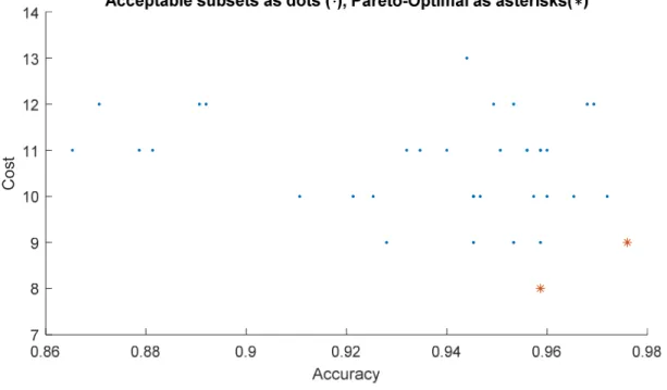
7. Representative Listing of the Ratio of cAFS/cPDS 107 8. The on-Frontier Ratio Across Selected Configurations 111 9. Cost Versus Features Used for POF for S 2 Dataset 113
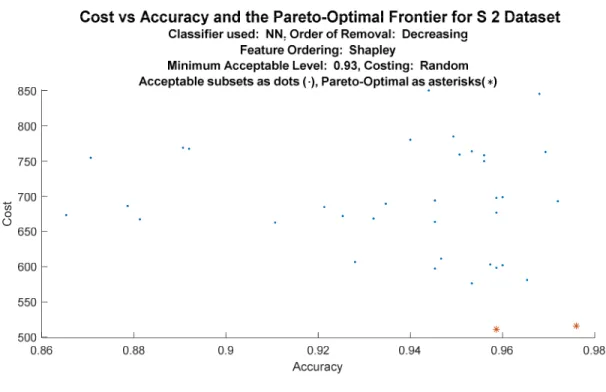
10. Cost Versus Features Used for POF for S 2 Dataset 114
11. Cost Versus Features Used for POF for Thyroid Dataset 116 12. Cost Versus Features Used for POF for Thyroid Dataset 117
13. Cost Versus Features Used for POF for Thyroid Dataset 118
14. Accuracy, Cost and Features Used for POF for the Indian Liver Dataset 119
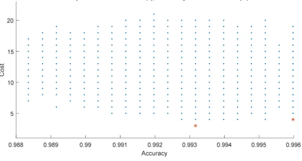
15. Accuracy, Cost and Features Used for POF for the WBC Dataset 121 viii
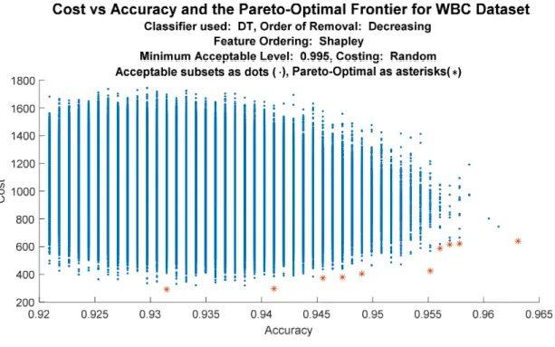
16. Accuracy, Cost and Features Used for POF for the WBC Dataset 121
17. POF When Cost of First Feature Decreased Decreased to 0.5 123 18. POF When Cost of First Feature Decreased Decreased to 0 123
19. POF When Cost of Specific Feature Increased to 10 124
20. The Relationship Between Feature and Frequency for WBC 126
21. Feature Importance for WBC, NNs, Decreasing Order 127
22. Comparison of Different Configurations on Resulting AFS and TST 129 23. Comparison of NN and DT Results for Similar Configurations 131
24. Synth Using Simple Ordering 147 25. Synth Using Shapley Ordering 148 26. S 2 Using Simple Ordering 149
27. S 2 Using Shapley Ordering 150 28. IL Using Simple Ordering 151
29. IL Using Shapley Ordering 153 30. Thyroid Using Simple Ordering 154 31. Thyroid Using Shapley Ordering 155
32. WBC Using Simple Ordering 156
33. WBC Using ShapleyOrdering 157
List of Figures
Figures
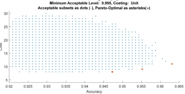
1. Pareto-Optimal Frontier for the S 2 Dataset. 113 2. Pareto-Optimal Frontier for the S 2 Dataset. 114
3. Pareto-Optimal frontier for theThyroid Dataset. 115 4. Pareto-Optimal Frontier for the Thyroid Dataset. 116
5. Pareto-Optimal Frontier for the Indian Liver Dataset. 118 6. Pareto-Optimal Frontier for the Indian Liver Dataset. 119 7. Pareto-Optimal Frontier for the WBC Dataset. 120
8. Pareto-Optimal Frontier for the WBC Dataset. 121
Chapter 1
Introduction
Background
Medical diagnosis is challenging and critical to safe and effective patient treatment. Successful diagnosis is often an iterative process beginning with an initial investigation, followed by some tests. Medical tests have several features. They all cost money. Many tests involve a level of discomfort or inconvenience for the patient while some are exceptionally painful or inconvenient. Many tests involve a measure of risk to the immediate or future health of the patient. In this description, tests have at least three dimensions of cost: dollar cost, pain or inconvenience cost and risk cost. The dollar cost may or may not be constant across all patients while pain plus inconvenience and risk may vary. Some people tolerate pain better than others, so the pain cost might be assessed differently by different patients. If a test causes an increased risk of cancer in 20 years, that risk might be meaningful to a 20 year old person, but much less so to an 80 year old person. The issue is that costs may vary from one situation to another.
The dollar cost may be borne by the individual patient or by another individual or group. Suppose that a clinic has an annual budget. When that budget is exhausted, the clinic can no longer function. It may be a simple if harsh reality that it is more effective to assess a large
number of patients with a slightly reduced accuracy rather than to assess a small number with a higher level of accuracy. In general, cost is a critical factor to consider.
Er, Yumusak, and Temurtas (2010) established that they could achieve high accuracy in diagnosing certain respiratory illnesses using an artificial neural network (NN). One feature on which they did not comment was the fact that every patient was given every one of 38 tests. It is possible that they might have achieved comparable results using fewer tests. If a trade-off between costs and accuracy can be established then a user will be in the position to make a better informed decision as to which features to measure.
This method can easily be generalized with respect to other classification objectives. Suppose an individual wants to decide which security (equity) to purchase (as Guresen, Kayakutlu, and Daim (2011) did). There are costs to gather different types of information and performance may vary depending on the information gathered. Suppose a researcher wants to detect disease in fish (as Gu, Deng, Lin, and Yu (2012) did), classify plants (as Yalcin and Razavi, (2016) did), or perform fault diagnosis (as Guo and Zhang (2008) did). Then the same general issues repeat. The best answer might be obtained with all features but there is a cost to collecting them; a lower cost, lower quality answer might be a better choice in some situations. Which choice should be made is not the focus of this effort. Rather, it is that the choices can be
associated with a specified level of accuracy and at a known cost. Providing the end user with the relationship between accuracy and cost allows the end user to be better informed and so make better decisions. This result can be obtained only if the accuracy versus cost relationship can be determined and that will be the primary focus of this investigation.
For purposes of this investigation, two separate classifiers will be utilized: neural
networks (NN) and decision trees (DT). The selection of these two is somewhat arbitrary as there are many other classifiers that might have been selected. However, both are represented broadly in the literature and the literature will be used to support their selection. The rationale for using a second type of classifier is to investigate whether or not the choice of classifier is relevant to the general process, described below.
Acceptable Results
While initially cast in the style of Er et al. (2010), these concepts can be generalized. Whether the question relates to diagnosing a patient, detecting disease in fish, selecting which security to purchase, or deciding any other question, the ability to determine an answer at an acceptable cost with an acceptable level of accuracy is critical. Resources are always constrained and better answers are always preferred. The trade-off between cost and quality of an answer is the critical feature of this investigation. The term ‘acceptable results’ will be used throughout this discussion. To some extent, this is a subjective term as it implies ‘acceptable to some party’ and that party may be under-defined. The specific values defining acceptable may vary depending on the party, the circumstances and the rationale for performing the classification.
Performance Measurements
There are several performance measures that will be used to evaluate the classifiers. A true positive (TP) is a case (instance in the test set) that was predicted to be true and actually was true. A true negative (TN) is a case that was predicted to be negative and actually was negative. A false positive (FP) is a case that was predicted to be true but was actually false. A false negative (FN) is a case that was predicted to be false but actually was true. Although these definitions apply to single instances, when used in formulas, as below, it is the count of the instances that is implied.
The total number of true samples is then TP + FN. Then the true positive rate (TPR) is defined as:
TPR = TP/(TP + FN).
The total number of false samples is then TN + FP. Then the true negative rate (TNR) is defined as:
TNR = TN/(TN + FP).
The false positive rate (FPR) is defined as: FPR = FP/(TN + FP).
The false negative rate (FNR) is defined as: FNR = FN/(TP + FN).
It is possible to eliminate some of these terms by noting (for example) that FNR = 1 – TPR or FPR = 1 – TNR.
The misclassification rate (MC) is the measure of items that were incorrectly predicted and is defined as:
MC = (FP + FN) / (total sample) = (FP + FN)/(TP + TN +FP + FN).
The overall classification accuracy rate (CAR) is the measure of items that were correctly predicted and is defined as:
CAR = (TP + TN) / (total sample) = (TP + TN)/(TP + TN +FP + FN).
(All definitions (Kelleher, Namee, & DArcy, 2015, pp. 404-414))
For purposes of this investigation, the CAR will be of primary interest. The author recognizes that this choice is somewhat arbitrary and that different users might have a different focus. It will be a trivial matter to adjust the process to focus on any accuracy measure which would have relevance to a given user.
Assume there are n features in a feature set FS. If the feature is present, then it is
represented by a 1 otherwise by a 0. It can be observed that for a given classifier, given a feature set FS = {F1, F2,…, Fn}, then the classifier will produce classification with some estimated level of
accuracy.
Each feature has some cost associated with it; call it Ci, for the ith feature. With a cost Ci
for each feature Fi the total cost if all tests are run is ∑(Ci * Fi) with Fi equal to 1 if the feature is
present and 0 if the feature is not.
Of note, the term “test” is used to imply generating the value for a feature. In terms of a medical classifier, the test would be the test performed on the patient; for other classifiers it would mean evaluating some feature.
With a feature set with n features there are 2n subsets so to test all subsets is infeasible for
even moderately large feature sets. For any given classifier it is a reasonable assumption that the ‘nearly’ best answer will be obtained using the largest set of features available. Removing a feature may have no effect (the feature does not contribute to the classification produced), or it may degrade the classification (the feature does contribute to the result), or in some cases, it may marginally improve the answer. Phrased differently, removing a feature from a feature set would
not be expected to materially improve the results obtained.1 (Aside: the removal of noisy features
may slightly improve the results, and this behavior was occasionally observed. The classifier will typically render such features as meaningless or nearly so. Further, as the threshold value to be used is in reference to the accuracy obtained with the complete feature set, if the accuracy is slightly higher for some subset there is no damage done to the overall assessment.) Therefore, beginning with a complete feature set, the task was to develop a method to remove some of the features without excessively degrading the overall performance of the classifier. That objective was the primary subject of this investigation.
If the costs of features were static it would have been possible to incorporate them early in the process. However, such an assumption could not have been justified. Costs may vary from person to person, time to time and situation to situation. Therefore, the incorporation of the costs had to be deferred until after the set of acceptable feature sets has been determined.
The level of accuracy for a given classifier was used in two ways. Suppose, after the removal of some feature, the remaining subset produced a level of accuracy that was unacceptable (a binary choice). That subset was rejected. Further, there was no further need to investigate any of the subsets of the rejected subset following from the assumption that removal of features does not improve the results. Suppose, instead, that the subset produced results above the specified accuracy threshold. Then that subset was included in the ‘acceptable’ set of subset and its subsets were tested for acceptability. The set of subsets that was determined to be acceptable was termed the Acceptable Feature Set (AFS). The actual level of accuracy was also used further. When the
1It is recognized that it may be possible to get an execution of a classifier that produces a superior
result with fewer features than does another execution using more features but that is simply due to the random nature of classifiers and the arbitrary assignments to training, validation and testing groups.
AFS was examined, clearly those subsets with a higher level of accuracy were preferred to those with a lower level. Hence, there was both a binary (acceptable or not) and a non-binary interest with respect to each acceptable subset.
Once the AFS was produced it was a trivial matter to evaluate the cost for each acceptable solution. At such time, the accuracy and the costs were matched and sorted both by cost and by accuracy. Producing a graph of cost versus performance was then a trivial matter. Of particular interest is the Pareto-Optimal Frontier, discussed below. The user could then select the optimal solution with respect to her situation.
Problem Statement
For any classifier, the cost of arriving at a decision may be a material issue. Collecting data is never a cost-free activity, and some data points can be exceptionally expensive. The cost component may have multiple dimensions (dollar cost, pain or discomfort, potential or actual risk or otherwise). It should be apparent that for any level of expenditure one would prefer the most accurate answer possible. Alternately, for any level of accuracy, the lowest expenditure would be most desirable. It is not difficult to extend this to a trade-off where accuracy and cost are in tension and can be made to describe an accuracy versus cost relationship.
Let , be a classifier for diagnosis trained on a set of input features using supervised machine learning method . Initially, let be constant. Then let ( , ) be the expected accuracy of , as determined by testing the trained model with respect to some accuracy measure . As noted, the TPR, TNR and CAR were of primary interest. Let Fmax be the set of all n features that might be used. Then the highest level of accuracy that could be expected would be
( , ). Unfortunately, this also results in the highest cost with respect to measuring the
input factors as all measures must be determined. Several observations were made:
1. Some attributes in Fmaxcontributed nothing to the estimate so could be eliminated without degrading the estimate.
2. The elimination of noisy features caused the accuracy to improve slightly. This does not invalidate the assumption that removing features tends to degrade the accuracy as the impact will be slight and may be zero if the classifier successfully renders their impact as zero.
3. It may be the case that some users would prefer lower accuracy if the
corresponding cost were significantly lower. A user could use the Pareto-Optimal Frontier to make an informed trade-off between accuracy and cost.
4. Unless a lower limit of acceptability is established, it would have been necessary to test all 2n - 1 combinations of features, which is infeasible. A lower bound on acceptability was established. For some datasets, the bound needed to be increased due to the very large number of feature subsets to be tested, especially when using random and increasing order of feature removal.
These were largely born out in the testing phase and are discussed further below.
Assumption:
⊂ then
Therefore, the problem was to identify all F* such that ∗, ≥ ! where ! is the accuracy threshold. Designate F* as the Acceptable Feature Set (AFS). Establishing a method to determine the AFS was the major effort of this investigation.
As the cost for each test would be assumed to be given, it would be trivial to calculate these corresponding costs. Furthermore, each Fi is also associated with its corresponding
( ", ).
Therefore, let {( Fi, ( ", ), #$( ", ))} with $ ∈ ∗ be the set of all acceptable
feature sets with the corresponding accuracy and costs. Ignoring the feature set itself we are left with
{( ( ", ), #$( ", ))}with $ ∈ ∗ which describes the accuracy versus cost relationship. Call this the Accuracy versus Cost Curve (AvCC). Since the accuracy of each trained model was established, the cost-accuracy tradeoff was obtained.
Dissertation Goals
The primary goal of the dissertation may be stated as follows:
Given an acceptable classifier , with respect to some minimum acceptable accuracy
thresholds ! for ∈ &, identify all subsets ' ⊂ such that (, are also acceptable. Call this set the Acceptable Feature Set (AFS).
Since the size | | of the feature set was large for some datasets, it was computationally infeasible to train and test classifiers using all 2| |− 1 subsets of features. We made reasonable assumptions to make the problem tractable:
Assumption: If a classifier (, is not acceptable, then all classifiers trained on a proper subset of
' are also not acceptable.
Assumption: There is a lower bound with respect to the accuracy below which the solution will not be of interest. This bound, ! , will be arbitrarily established. It establishes a threshold level above which the estimated accuracy is acceptable while below which the estimated accuracy is not acceptable. (Aside: the threshold level also had a material impact on the number of subsets that were evaluated. Hence, the threshold level was altered to be materially higher than initially planned for some datasets.)
Assumption: A ‘nearly best’ answer was obtained by using all of the features. Some results did improve slightly as some noisy features were removed. However, the assumption was that
accuracy will soon start to fall off as more meaningful features are removed. Stated differently, if a subset of features produced an accuracy below the threshold level, then any subset of that subset would also be below the threshold level.
Assumption: Features can be ranked in a meaningful order (least to most significant or the reverse). Any such ranking is somewhat subjective as the methodology used to establish significance is a user choice (although once the choice is made there would be no further subjectivity). Several different approaches to ranking were employed, discussed below.
Under these assumptions, this dissertation applied depth first tree search to identify all subsets of that result in acceptable classifiers. Nodes were represented by the feature set used to train and test the model. The root node was represented by the full feature set Fmax. For a node represented by feature set ', a set of | '| successor nodes was obtained as * '− * +| ∈ '+ by removing one feature at a time. Nodes representing classifiers that are not acceptable are removed
from the search tree and its subsets were never considered; all nodes remaining in the tree were acceptable classifiers.
A secondary goal of this dissertation was to investigate whether a judicious choice of the order in which features were removed could reduce the total number of classifiers to be trained and tested, thus reducing the total time needed to identify the set of acceptable classifiers. The set of acceptable feature sets was designated as the Acceptable Feature Set (AFS).
The relative importance of features in a classifier may be estimated. Our hypothesis was that the total number of nodes in our search tree could be reduced by considering a successor node obtained by the removal of a relatively more important feature before a successor node obtained by the removal of a relatively less important feature. This dissertation investigated this hypothesis by removing features in three different orders to generate successor nodes: descending, random, and ascending order of relative importance.
A tertiary goal of this dissertation was to demonstrate the practical benefits of identifying all acceptable models. For each acceptable classifier, its accuracy profile was presented in terms of all accuracy measures ∈ &. The cost associated with applying a trained classifier , for diagnosis may be taken to be the sum of the cost of obtaining values for its input feature set . Let ,$ be the cost of obtaining a sample value for feature . Then the cost of applying , for
diagnosis may be computed as #( , ) = ∑$∈ ,$.
The cost of applying an acceptable classifier with feature set ' for diagnosis is #( (, ) = ∑$∈ ,$
( . Using these costs, a non-dominated set of classifiers in the Pareto-Optimal Frontier of the cost-accuracy space was obtained. Decision makers could make informed decisions regarding the test results by selecting a subset of features used by some model in this
frontier. The set of acceptable classifiers and the corresponding accuracy profiles will be established. This will be referred to as the Accuracy versus Cost Curve.
The final goal was to determine the performance of DTs as compared to NNs. The resources required to execute the AFS was a primary area of interest. Also, the actual AFSs produced were compared. Of note, this was not to be construed as a validation of either DTs or NNs for classification as both are well supported in this role in the literature.
Research Questions
Research Question 1: What is an efficient process to identify all acceptable feature sets?
This question required developing a method to reduce the feature set by removing features one at a time, producing a subset, and then evaluating the result of that subset. If the result was at or above the acceptable level, then the feature set of that subset was included in the AFS. If it was acceptable, then its children were also evaluated. If it was not acceptable, then it was not included in the AFS and its subsets were ignored using the assumption that removing a feature does not improve the classifier’s results.
Here, the term ‘subsets’ is used in the following sense. Suppose the current feature set is {1,1,1,0}, with the usual convention of 1 indicating the feature is present and 0 indicating that it is not. If we consider the rank (Rs) of each set to be the count of the number of 1s present then the
rank of each of that set’s subsets is Rs – 1. It was never the case that a feature is added back when
producing the subsets. The initial (top level) set was that with all features present and the features were removed one at a time. The top level set then has rank n, with n the number of features. Therefore, the subsets of {1,1,1,0} are {{0,1,1,0}, {1,0,1,0}, and {1,1,0,0}}. Specifically, each
feature that was present (a ‘1’) was removed in turn. (Note, the set representation does not reflect how the features will be coded, merely how they are conceptualized.)
Research Question 2: What percentage of the reduced feature sets are above the minimum quality threshold established?
This was a simple count of the AFS compared to the total possible number of subsets. The count increased as the threshold of acceptability was decreased.
Research Question 3: What percentage of the qualifying feature sets are on the Pareto-Optimal Frontier?
Answering this question required determining the Pareto-Optimal Frontier then comparing that with all of the AFS. This determination was relatively straight-forward once the AFS had been established.
Research Question 4: Does the order in which features are removed have an impact on the number of expansions required?
Answering this question required testing the implementation with different orders of removal. That is, the removal can be based on most significant first, least significant first or random order.
Research Question 5: What is the impact of using a different classifier on the AFS produced and the overall efficiency of the process?
This question was addressed by swapping the Neural Network classifier for the Decision Tree classifier. A simple comparison of the number of expansions produced one dimension for
comparison. A more interesting comparison was the actual feature sets produced for a given level of accuracy.
Relevance and Significance
Problem and those impacted
Cost is always a consideration in any activity. Quality of performance is also significant in most activities. Frequently, these two concerns are in tension. Better performance can often be obtained at a higher price. A lower price can typically be obtained by sacrificing the quality of the answer produced. This tension is obvious in many systems.
The cost of obtaining a specific feature is not necessarily indicative of how much that feature contributes to the quality of a decision. When the number of tests that might contribute to the quality of an answer increases, it becomes infeasible to evaluate all of the combinations of tests that might be used. Therefore, a heuristic is required to select the ones to use. There is no well-defined method to address that issue, especially when the costs of the tests are considered. Further, if the costs are dynamic, an additional layer of complexity is introduced to the general question.
The purpose of this investigation was to determine if there is a feasible method of reducing the search space to produce a lower cost answer of acceptable quality. Neural Networks were used as the evaluation criteria, but many other methods could have been used instead of them, for instance, decision trees, support vector machines or Naïve Bayes could also have been used. The rationale for using NNs was arbitrary but not capricious. They have a long history of being used for decision making or as classifiers and they have been shown to provide reasonably accurate results. The literature has numerous instances of NNs being used as classifiers in medical
diagnoses and in many other areas. While NNs were the primary classifier used, DTs were used as a confirmation that the results are not tied tightly to the choice of classifier. This confirmation will allow others to employ the classifier of their choice.
With respect to medical diagnoses, as well as the other items mentioned in the literature review and elsewhere in this document, Neural Networks have been used for diagnosing many things including:
• eye disorders (Syiam, 1994),
• ovarian cancer (Tan, Quek, & Ng, 2005),
• cirrhosis (Sun, Lu, Kobayashi, & Yahagi, 2005),
• carpal tunnel syndrome (Palfy & Papez, 2007),
• sleep apnea (Marcos, Hornero, Alvarez, Campo, & Lopez, 2007),
• macular diseases (Luculescu & Lache, 2008),
• Alzheimer’s disease (Huang, Yan, Jiang, & Wang, 2008),
• thyroid disorders (Shukla, Tiwari, Kaur, & Janghel, 2009),
• endometrial cancer (Xiang, Tian, Zhang, & Dai, 2009),
• psychiatric disorders (Cui, Xiong, Zheng, & Chen, 2012),
• malnutrition related diseases (Arista-Jalife & Arista-Viveros, 2012)
• liver cancer (Kondo, Ueno, & Takao, 2012),
• flat footedness (Aruntammanak, Aunhathaweesup, Wongseree, Leelasantitham, & Kiattisin, 2013),
• stroke (Lin, Hsieh, & Hu, 2013),
• multiple sclerosis (Gutierrez, 2015)
• Parkinson’s disease (Bazgir, Frounchi, Habibi, Palma, & Pierleoni, 2015),
• hypertension (Pytel, Nawarycz, Drygas, & Ostrowska-Nawarycz, 2015),
• prostate cancer (Sammouda, Wang, & Basilion, 2015),
• gum disease (Thakur, Guleria, & Bansal, 2016), and
• congenital heart septum defects (Jyothi & Vanisree, 2016).
Outside of medical diagnosis, neural networks have also found material application. Specifically, NNs have been successfully used in:
• fault diagnosis for steam turbines (Guo & Zhang, 2008),
• processing natural language (Collobert & Weston, 2008),
• stock market prediction (Guresen, Kayakutlu, & Daim 2011),
• detecting disease in fish (Gu, Deng, Lin, & Yu, 2012),
• predicting the strength of high performance concrete (Venu, Kiran, & Kiranmai, 2012),
• detecting disease in plants (Dhakate & Ingole 2015),
• fault diagnosis in lithium-ion batteries (Gao, Chin, Woo, Jia, & Toh, 2015),
• selecting recommendations for viewers on YouTube (Covington, Adams, & Sargin, 2016),
• plant classification (Yalcin & Razavi, 2016),
• automatically processing photographic enhancements (Yan, Zhang, Wang, Paris, & Yu, 2016), and
Similarly, decision trees have been used in such medical diagnoses or treatment situations as:
• anemia (Maity, Sarkar & Chakraborty, 2012),
• bladder cancer (Floares & Birlutiu, 2012),
• monitoring posture and activities (Zhang & Sazonov, 2012),
• pulmonary disorders (Tartar, Kilic & Akan, 2013),
• Alzheimer’s disease (Al-Dlaeen & Alashqur, 2014),
• brain tumor (glioblastoma) (Chaddad, Zinn & Colen, 2014),
• cardiovascular dysautonomias (Kadi & Idri, 2015),
• heart failure (Aljaaf, Al-Jumeily, Hussain, Dawson, Fergus and Al-Jumaily, 2015),
• thyroid disease (Shroff, Pise, Chalekar & Panicker, 2015),
• liver fibrosis (Ayeldeen, Shaker, Ayeldeen & Anwar, 2015),
• monitoring pregnancy (Lakshmi, Indumathi & Ravi, 2015),
• cerebral hemorrhage (Kumar & Krishniah, 2016)
• diabetes (Songthung & Sripanidkulchai, 2016), and
• breast cancer (Al-Salihy & Ibrikci, 2017).
Outside of medical diagnosis, decision trees have also found material application. Specifically, DTs have been successfully used in:
• detecting failure in internet sites (Chen, Zheng, Lloyd, Jordan & Brewer, 2004),
• network intrusion detection (Stein, Chen, Wu & Hua, 2005),
• identifying imposters on social media (Fong, Zhuang & He, 2012),
• detecting fraud (Zou, Sun, Yu & Liu, 2012),
• stock trading (Ochotorena, Yap, Dadios & Sybingco, 2012),
• identifying individuals using biometric based identification (Kumar, Hanmandlu, Das & Gupta, 2012),
• security assessment of power systems (He, Zhang & Vittal, 2013),
• human gesture recognition (Oh, Kim & Hong, 2013),
• packet classification (Cheng & Wang, 2013),
• recognizing emotional aspects of speech (Yuncu, Hacihabiboglu and Bozsahin, 2014),
• detection of suspicious emails (Sharma, 2014), and
• assessing wine quality (Lee, Par, & Kang, 2015).
These lists were not meant to be exhaustive, merely illustrative. A simple search in the ACM on-line library for ‘neural network’ returned over 3700 hits. NNs are widely used in a variety of settings. The purpose of this investigation was neither to assert that NNs are the only or best choice for the evaluation portion nor to provide yet another example of using NNs for
decision making. Rather, the purpose was to utilize NNs as a well-established tool to evaluate the heuristics proposed. So, the use of NNs was arbitrary, but considered. The same considerations apply for DTs.
Of note, this investigation made no effort to determine how the costs are generated. Nor was it concerned with which components of cost are considered. In an actual implementation, the costs would be sourced from others. In this investigation, costs were generated synthetically.
Scope of the problem, impact and benefit of a solution
Deciding how to classify items, situations, events or conditions is an exceptionally general problem. One might wish to categorize a disease. One might wish to determine which equities will perform better than others. One might wish to determine the species of a plant. One might wish to determine the effectiveness of various types of treatments. One might wish to determine the best time to plant or harvest a crop. The number of situations in which one might wish to determine an answer to a categorization problem is almost endless. For all of these questions, inputs must be provided. To test, that is, determine the value of, each input incurs some cost. The cost may be measured along a number of axes (dollar cost, inconvenience/pain, potential or actual risk, or some other dimension). The objective is not to list every potential dimension of cost but rather to note that there are many and these may vary from determination to determination, situation to situation, or person to person.
Costs are a concern in every environment. Resources are limited. The quality of a decision can frequently be improved by increasing the tests performed and so increasing costs. Eliminating some tests decreases the cost but may also degrade the quality of the answer obtained. This is an essential tradeoff. The point of this investigation is to determine exactly what that tradeoff curve looks like. Being able to utilize the AvCC for decision making would have potential value in any situation where a categorizer of any sort is being used.
It could be argued that there is a simpler way to approach this problem. That is, when the complete feature set is considered, simply remove each feature one-by-one, assess the change in accuracy and then use that information to guide the feature reductions. While that might produce acceptable results under some circumstances it would not be a general solution. Consider a situation where the subject’s weight happened to be recorded in both pounds and kilograms.
Eliminating either of those should have no effect on the classifier. The researcher might reasonably conclude that neither were required and eliminate both of them. Data might, and almost certainly would, interact in more complex and subtle ways. Therefore, the single
elimination/evaluation is inadequate. If the solution were extended to two-at-a-time removals and then three-at-a-time the number of cases required quickly expands. As there is no sound reason to stop at any number, the solution very rapidly becomes an exhaustive search which is infeasible.
Previous research and consequences of leaving the problem unsolved
While there have been attempts to address costs in categorizers, the attempts have not addressed the general issue of cost reduction related to feature elimination. Rather, the attempts typically address a particular problem and find a unique solution to that problem.
Vijayasarveswari, Khatun, Jusoh, Fakir, and Ali (2016) utilized a NN in the analysis of breast cancer. Their approach keyed on utilizing less expensive hardware to perform the tests required. While effective, it is not a generalizable approach (leaving aside the notion that if there is cheaper hardware that suffices it makes sense to use that instead). Seo, Yu, Lee, and Choi (2016) considered the overhead of running very large NNs and proposed modifications to the way in which inputs were categorized as a potential solution to this problem. While they
acknowledged the cost of running the networks, they did not address the costs of obtaining the input values themselves.
Ji, Jiang, Zhao, and Zhai (2015) proposed a method of discriminating on the value
provided by the tests used in their NN but did not address the cost component of the tests. While the value of a test is certainly of interest, the cost of obtaining that value must also be a concern.
Some work has been done that recognizes that costs are a factor or that reducing costs is generally desirable. However, with respect to directly assessing costs of obtaining the value of input parameters and using that information as a way to reduce costs, no work has been observed in this area. Therefore, this effort represents an investigation into an unexplored segment of decision making.
The consequences of solving this problem, even partially, could be quite significant. Every test performed consumes resources. In an environment where only the best answer is acceptable, a needless test simply wastes resources. In an environment where resources are constrained, spending those resources sub-optimally means that other investigations are foregone, whether immediately or at a later date, or that suboptimal conclusions may be produced. The effective use of testing resources will either save resources, improve the quality of the results obtained, or possibly both.
Addressing the research problem and potential for success
This study addressed the issue of cost in two distinct forms. The ultimate goal is to generate the AvCC which will allow a user to select the best choice for their situation, given that the user can define ‘best’ however desired. This first item has been the ultimate driver, but it was trivial to calculate once the AFS had been generated. The more difficult issue was the cost of finding the AFS. Given limitless time and resources, a brute force method would, eventually, produce a result which should match the AFS given that the assumptions stated elsewhere remain valid. However, limitless time and resources are not feasible. Hence, it was ultimately the cost of finding the AFS in a cost effective manner that was of concern.
The method proposed eliminated large branches of the search tree early in the pruning stage. Such early pruning vastly reduced the number of combinations that needed to be evaluated. The reduction was sufficient such that the time and resources required would be feasible in a wide variety of situations. Further, this study examined the impact of altering the selection for removal order (most significant feature, least significant feature, random feature). The most efficient removal order was to remove the most significant feature first was the most costly order was to remove the least significant feature first.
The pruning process described did produce an answer in less time than the brute force method would require. The issue then reduces to whether or not the speed-up was sufficient to justify the effort required. To a large extent this issue hinged on the minimum acceptance level that was selected. If the minimum was chosen close to the maximum, then even a modest loss of information (removal of only a few features) was sufficient to degrade the answer to the point where it was not acceptable. Therefore, the tree might have been pruned after only a few
removals. The total number of subsets searched would have been a small multiple of the number of features. However, when the minimum acceptable answer was set very low, the classifier could produce a large number of acceptable, if less accurate, answers with only a small number of features. In these cases, the tree would have been pruned only after a large number of features were removed and there were many such nodes. The number of subsets considered was frequently very large and the resources required were significant. As it transpired, for several datasets the number of nodes tested was very high even when the threshold level was relatively close to the maximum value.
Adding to the knowledge base
This research added materially to the understanding of how costs can be used to influence the selection of features to be used in decision making. In every case where decisions are being made, there is a cost with determining the results. Costs are always a constraining factor, whether they are explicitly recognized as such or not. With this research concluded, the author can now provide a user with a process by which the contribution of a test to a determination can be evaluated. Cost-effective features can be included in the test suite. Cost-ineffective ones can be eliminated. Further, the user will have the ability to examine the AvCC to determine how best to deploy scarce resources. This method has demonstrated that it can readily accommodate dynamic costs.
Through this investigation, an understanding of how various factors impact the cost of generating an AFS was gained. This understanding will allow a user to generate a new AFS efficiently. As there are many classification problems and virtually all of them require inputs of varying costs, this understanding may provide wide-spread benefit.
Additionally, suppose a new feature is suggested for the test suite. A user now has the ability to evaluate whether to include the feature or not. A medical diagnostician may also be able to determine that, if the cost is less than a certain amount, then it should be included, otherwise not. Alternately, an individual suggesting (perhaps selling) the new test might be able to determine the ideal price to charge to obtain the maximum profit for that test. The decision making process will be improved.
Additionally, knowledge will be gained regarding the impact of lowering the acceptability threshold. As the level is decreased, the number of acceptable feature subsets increased
dramatically. By measuring the effort required to solve problems of a different sizes, insight was gained into the size of problems for which this approach is suitable.
Potential for generalization
The initial impetus for this investigation was to study the removal of select tests from a test suite which was the input to a NN being used to categorize specific diseases. It is apparent that different tests may have dramatically different costs. It is also apparent that different tests will have different impacts on the results returned by the NN. It is possible that in some environments, the limiting factor in selecting which tests to use would be obtaining the best performance (that is, highest accuracy possible). Still, there might still be opportunity for cost reduction if some tests might be found to provide no useful information. However, as the level of acceptable
performance is lowered, the opportunity to reduce cost increases. One might argue that when performing a diagnosis, only the best available performance is acceptable, however that is not necessarily the case. Consider a case where disease A and B both have comparable treatments. In such a case, it may not make good sense to spend limited resources to differentiate between the two (provided that one can be satisfied that it is either A or B and not something else). Further, not all environments are rich enough to support exhaustive testing. There may not be enough trained individuals to perform all of the tests; the materials required to perform all of the tests may not be available (or affordable); some tests may pose excessive hazards or cause pain to some or all patients; or the patients themselves may not be able to make visits to the places where certain tests are to be carried out. So, it may be the case that one can perform a very small number of diagnoses with a high level of accuracy or a much larger number with a slightly lower level of accuracy. The interaction of these relationships can all be revealed with a suitable AvCC.
While it is a trivial matter to describe an algorithm that will test every combination of tests (and so build an exact cost for each subset of tests) it is infeasible to run such a process for even modest sized feature sets. As noted elsewhere, the run time is proportional to 2n - 1, with n the
number of tests. For each test, a NN, or other classifier, must be generated. The run times are simply not feasible for even moderately large values of n. Therefore, the methods described in this paper were developed. These methods have been tested and found to be satisfactory; the potential for generalization is significant. There are many comparable systems that use NNs or other classifiers to assist with a decision. Being able to efficiently generate a new AvCC given a different set of costs would allow the users of such systems to be more informed as to the value their systems would generate.
Neural Networks were designated as the primary classifier for this investigation, with decision trees as the confirmation classifier. That choice was arbitrary. Using a NN was
convenient because there are many pre-packaged environments that are readily available (e.g. R, Matlab). Further, NNs and DTs have been used in so many classification systems that there is a high level of confidence that they actually do work correctly and effectively. However, any process that uses inputs to make a decision would have sufficed (e.g. Support Vector Machines, Naïve Bayes classifiers). It is not the decision making process that was being examined, rather the method to extract an appropriate subset of the input tests. Therefore, there is additional potential for generalization with respect to the type of classifier used.
From the above discussion, it is not difficult to conclude that this work can be generalized. There are a significant number of NN and DT systems that are used and benefit could be gained from understanding the cost/accuracy tradeoff. Further, it is trivial to swap out the NN classifier and substitute a different classifier.
Potential for original work
While it is not uncommon to see those writing about classifiers mention cost as an issue, there is negligible evidence that cost has been researched to any material extent. Further, dollar cost is frequently a proxy for many other measures. Humans put a dollar cost on property, on opportunity, on inconvenience, on discomfort, on risk, and on many other things. These costs may not always be explicitly stated (or precisely measured), but that does not mean they are not real. It is not difficult to imagine many situations where one might put a dollar cost on things that are normally measured in other terms. The person who pays extra to drive on a toll road implies a dollar cost for convenience (or time saved). The person who pays extra to sit in a first-class airline seat implies a dollar cost for comfort. The person who pays extra for safety features in an
automobile implies that money can be exchanged for safety. The number of examples of trading money for something else would be almost endless and the objective is not to provide an
exhaustive list of such exchanges, simply to note that such exchanges are common.
Therefore, with the potential to measure many items of value in terms of money, one can begin to examine a more extensive trade-off. When there are dozens or perhaps hundreds of terms involved, the utility of a common currency should become apparent. Further, not all individuals will place the same value on certain elements. A procedure that would make an individual sterile would be of no consequence to a 90 year-old person but might be devastating to a 20 year-old one. An investigation that would degrade one’s physical performance in a foot race by two percent would not be meaningful to most individuals but might be catastrophic to a professional athlete. A procedure that cost $1,000 might pose an unbearable burden to one person, yet be a trivial amount to another. Costs may be exceptionally dynamic and completely person specific.
Most of these implications have not been explored. While it is trivial to look up an example of NNs or DTs being used as an aid in medical diagnosis or to investigate other categorization problems (see section: Relevance and Significance), costs are not normally a consideration. This effort presents an investigation into an area that has been neglected.
Barriers and Issues
It is not a trivial task to perform a diagnosis. Acquiring and organizing the data needed to train a neural network or other classifier may present a material challenge and a significant cost. Although it is evident that neural networks and other classifiers can be trained to diagnose
accurately in many cases, the issue of the cost of acquiring the data for the diagnosis has received scant, if any, attention. Part of the reason for the lack of attention may be that there has been no method developed to understand the relationship between cost of a particular test and the benefit of that test, particularly when combined with other tests. This study is focused on the relationship between accuracy and cost and can only do that by understanding the collective value of subsets of the feature set when taken together.
The principal difficulty in approaching this problem is that there is no known relationship between the features. That is, one cannot isolate the contributions of each feature. The
relationship between a collection of features and the resultant accuracy of the classifier where there will be multiple features present is simply not known from their individual contributions.
Therefore, the only currently practical way to determine the relationship is to test the various combinations. For feature sets of more than a modest cardinality, the task of computing all combinations is simply infeasible. Therefore, some simplifying techniques or assumptions must be applied. The simplifying assumption that was employed in this study is that if a feature is
removed from a feature set, the accuracy of the classifier does not go up materially. Phrased differently, if a subset of features falls below the acceptable level, removing a feature will not result in an acceptable subset. That concept was used to reduce the infeasible brute-force method to a manageable one.
As remarked elsewhere, there are a great number of areas in which categorization is a material concern. For virtually all such situations, cost is a material factor. Therefore, obtaining the accuracy/cost curve for categorizing a problem in a timely manner is both challenging and valuable. The general solution will be initially cast as a solution to a medical diagnosis problem. However, there is nothing in the concept of classifier or costs that is peculiar to medical diagnosis so the solution will have general applicability.
Assumptions, Limitations and Delimitations
The assumptions below have been introduced elsewhere in this paper. They are included here for completeness.
Assumption: If a classifier (, is not acceptable, then all classifiers trained on a proper subset of
' are also not acceptable.
Assumption: There is a lower bound with respect to the accuracy below which the solution will not be of interest. This bound, ! , will be arbitrarily established. It establishes a threshold level above which the estimated accuracy is acceptable while below which the estimated accuracy is not acceptable.
Assumption: A ‘nearly best’ answer will be obtained by using all of the features. The results might improve slightly as some noisy features are removed. However, the assumption is that accuracy will soon start to fall off as more meaningful features are removed. Stated differently, if
a subset of features produces an accuracy below the threshold level, then any subset of that subset will also be below the threshold level.
Assumption: Features can be ranked in a meaningful order (least to most significant or the reverse). Any such ranking is somewhat subjective as the methodology used to establish significance is a user choice (although once the choice is made there would be no further subjectivity).
There are no apparent limitations other than that the number of evaluations increases dramatically as the number of features increases. Of note, the calculation of the AFS need only be done once for a given set of features, it does not need to be repeated when the prices are updated. The only delimitations are those related to the choice of datasets. That is, it is necessary to use actual datasets, hence the choice is arbitrary, regardless of who actually makes the choice.
Definition of Terms
All of the following items are also included in the List of Acronyms. Most of the acronyms are common terms that are frequently used. The few that are detailed here are not commonly employed but are specific to this investigation.
ACC0 (initial accuracy) is the initial accuracy of the classifier. Given a classifier and a
complete set of features, the classifier will produce an accuracy of ACC0.
The Acceptable Feature Set (AFS) is the set of all subsets of features that, using a given classifier, produce a level of accuracy equal to or above the threshold level.
The Accuracy versus Cost Curve (AvCC) is the relationship between accuracy obtained and the cost of obtaining that accuracy. Ultimately, it is the goal of this investigation.
List of Acronyms
The following Acronyms have been used in this paper:
• ACC0: Initial accuracy of the classifier • AFS: Acceptable Feature Set
• AvCC: Accuracy versus Cost Curve
• cAFS: count AFS
• cFST: count Failed Sets Tested
• cPOF: count of sets on POF
• cPDS: count of Potential Data Sets
• cTST: count Total Sets Tested
• CAR: Classification Accuracy
• DT: Decision Tree
• NN: Neural Network
• FN: False Negative
• FNR: False Negative Rate
• FP: False Positive
• FPN: False Positive Rate
• MC: Misclassification Rate
• TN: True Negative
• TNR: True Negative Rate
• TP: True Positive
Summary
Medical diagnosis is a challenging and expensive task. There are many examples of NNs and DTs being used for medical diagnosis as well as for other decision making efforts. Not all features will necessarily contribute meaningfully to the accuracy of a classifier. All features have a positive cost related to their collection. These costs may exist in multiple dimensions (actual dollar cost, inconvenience or discomfort, potential health risks or other) but can be reduced to a dollar cost.
Reducing the features employed generally reduces the accuracy but also reduces the cost of the assessment. Therefore, it is easy to consider a relationship between the cost of producing an answer and the anticipated accuracy of that answer. This relationship is the essential focus of this investigation.
This study succeeded in finding the relationship between features measured and accuracy for several specific datasets. This was done by establishing a minimum acceptable accuracy then generating all of the subsets of features that meet or exceed that accuracy level. It is assumed that the ‘nearly’ best answer is achieved when all features are present. As features were removed, the accuracy of the answer deteriorated. It was also assumed that, below a certain level of accuracy, an end user would have no interest in the answer.
Hence, it was easy to establish two bounds. The upper bound of accuracy was the value obtained when all features are present. Whether the accuracy improves slightly with the removal of ‘noisy’ features is of little consequence. The lower bound of accuracy is the lower limit at which a user might be interested in the answer. Between those two values, all subsets of features are of interest. It was the objective of this investigation to find them in an efficient manner and
then present them as a Pareto-Optimal Frontier. Then end user would then be able to apply any dynamic cost function to the frontier to determine their optimal course of action.
Chapter 2
Review of the Literature
There are eight areas of particular interest in this literature review. The first area is to examine the support for using Neural Networks as the classifier. The goal is to demonstrate that NNs have a long history of being used to accept input factors and produce a classification. The classification might be a simple binary situation (e.g. to determine if this is a buying opportunity or not, or to determine if a tumor malignant or benign). Alternately, the classification might be to determine which of several choices is best (e.g., to determine if the patient has disease A, B, C, or D).
The second area of interest is to highlight that very little effort has been put into studying the impact of costs on a diagnosis. While it is not possible to show that no effort has been
expended to examine costs (one would have to examine all papers produced, which is infeasible), it is possible to review a material number and comment as to whether or not minimizing cost via selection of factors was a non-trivial component of the study.
The third area will be to establish that decision trees are also an established classifier for performing diagnosis. The second type of classifier is desired to establish that the process is not
tightly tied to neural networks. That is, any classifier of choice could be selected and the process should still be valid.
Of note the first three areas of interest are considered together. They form the first subsection of the literature review.
The fourth area of interest is to review active versus passive classifiers. Greiner, Grove, and Roth (2002) discussed costs in the context of an active versus a passive classifier.
The fifth, sixth and seventh areas all relate to feature set reduction. The articles selected represent some of the early work performed in this area and have been referenced many times in the literature. Hence, they represent key early developments. In the fifth section, reduction using the filter method is reviewed. In the sixth section, early work on the wrapper method is discussed. In the seventh section, the hybrid method is reviewed. These seminal efforts will be traced
forward to the present.
For each study discussed, remarks will be produced as to the nature of the study and the results obtained. Further, the extent to which cost was considered will be noted.
The eighth section will summarize the current state of affairs. It will largely follow the organization of Li et al. (2017), but will also incorporate other elements.
Neural Networks, Decision Trees and Cost Considerations
Er, Yumusak, and Temurtas (2010) noted that neural networks had been used previously for respiratory and other medical diagnoses. These 3 researchers worked (not always together and frequently with others) on 7 of the 37 papers used as reference material for their article. Further, they referenced that paper in four later articles. This specific article can be viewed as one in an
ongoing series where they (and many others) delve into this topic. They used a variety of NNs to diagnose respiratory illnesses. They considered several different types of NNs including multi-layer neural network (MLNN), probabilistic neural network (PNN), learning vector quantization (LVQ) neural network, generalized regression neural network (GRNN) and radial basis function (RBF) neural network. These were used to produce a differential diagnoses between TB
(tuberculosis), COPD (chronic obstructive pulmonary disease), pneumonia, asthma, lung cancer, and no illness present. Their dataset used 38 input features. They used Matlab for their
calculations. Accuracy varied from 88% with GRNN to 92% with PNN. There was no discussion of costs.
El-Solh, Hsiao, Goodnough, Serghani and Grant (1999) described using Neural Networks to diagnose tuberculosis. They reported that their methods (General Regression Neural Network (GRNN)) outperformed physicians' clinical determinations. There was no discussion of costs.
Kabari and Bakpo (2009) developed a neural network which was successful in
diagnosing selected skin diseases. They reported performance in excess of 90% accuracy. They mentioned that costs were a factor but did not follow through with any analysis of the cost of tests. They did remark that NNs may help reduce costs, but did not elaborate on the details of how this might be achieved.
Vijayasarveswari et al. (2016) proposed a NN solution for screening for breast cancer. They reported accuracy ranging from 82% to 100%. Their method did consider feature reduction, but it was an across the board effort; it was not selective to individual circumstances. The authors did note that their system was materially less expensive than others, but it was designed as a replacement for a more sophisticated system. It did not use the evaluation of the tests used by the
NNs as a method to choose between various tests. Rather, it was completely a one-off resolution; their contribution was designing a less expensive replacement of a more expensive system.
Ibrahim, Shamsuddin, Saleh, Abdelmaboud, and Ali (2015) used a multilayer perceptron with differential evolution technique to produce NNs used in the diagnosis of breast cancer. They used the University of Wisconsin Hospitals, nine parameter dataset (available at
https://archive.ics.uci.edu/ml/datasets/Breast+Cancer+Wisconsin+(Original)). They commented that “The multi-objective evolutionary algorithm used in this work optimizes error rates and architectures of the MLP network simultaneously” (p. 424). Overall, they reported accuracy rates averaging 97.51%. There was no discussion of costs.
Liu and Dong (2012) also used NNs to diagnose breast cancer using the same Wisconsin Hospital data as did Ibrahim et al. (2015). They used the Levenberg-Marquardt algorithm instead of the Gradient descent algorithm. The rationale stated was that “L-M algorithm uses the
approximate information of the second derivative, and is much faster than gradient method” (p. 1239). They reported an accuracy rate of 98.8%. There was no discussion of costs.
Chunekar and Ambulgekar (2009) applied neural networks to three different datasets to diagnose breast cancer. They reported accuracy ranging from 70.7 to 98.8% which supports the notion that NNs can be useful for diagnosing. Of note, the relatively low 70.7% result was not explained. They did remark that “these neural network based clinical decision support systems avoid unnecessary excision and expense” (p. 895) which, at a minimum, recognized that pain and expense are factors that might be considered. However, it was within the general context of using NNs instead of (or in support of) other methods. No analysis of the cost of the tests used in the NNs was discussed.