Deep Shape Representations for 3D Object Recognition
Hamed Ghodrati Asbfroushani
A Thesis in
The Concordia Institute for
Information Systems Engineering
Presented in Partial Fulfillment of the Requirements For the Degree of
Doctor of Philosophy (Information and Systems Engineering) at Concordia University
Montreal, QC, Canada
October 2017 c
CONCORDIA UNIVERSITY SCHOOL OF GRADUATE STUDIES This is to certify that the thesis prepared
By: Hamed Ghodrati Asbfroushani
Entitled: Deep Shape Representations for 3D Object Recognition and submitted in partial fulfillment of the requirements for the degree of
Doctor of Philosophy (Information and Systems Engineering) complies with the regulations of the University and meets the accepted standards with respect to originality and quality.
Signed by the final examining committee:
________________________________________________ Chair Dr. Rabin Raut
________________________________________________ External Examiner Dr. Prabir Bhattacharya
________________________________________________ External Examiner to Program Dr. Hassan Rivaz ________________________________________________ Internal Examiner Dr. Jamal Bentahar ________________________________________________ Internal Examiner Dr. Nizar Bouguila ________________________________________________ Thesis Supervisor Dr. Abdessamad Ben Hamza
Approved by ______________________________________________________________ Dr. Chadi Assi, Graduate Program Director
October 23, 2017
______________________________________________________________ Dr. Amir Asif, Dean, Faculty of Engineering and Computer Science
Abstract
Deep Shape Representations for 3D Object Recognition Hamed Ghodrati Asbfroushani, Ph.D.
Concordia University, 2017
Deep learning is a rapidly growing discipline that models high-level features in data as multilay-ered neural networks. The recent trend toward deep neural networks has been driven, in large part, by a combination of affordable computing hardware, open source software, and the availability of pre-trained networks on large-scale datasets.
In this thesis, we propose deep learning approaches to 3D shape recognition using a multi-level feature learning paradigm. We start by comprehensively reviewing recent shape descriptors, including hand-crafted descriptors that are mostly developed in the spectral geometry setting and also the ones obtained via learning-based methods. Then, we introduce novel multi-level feature learning approaches using spectral graph wavelets, bag-of-features and deep learning. Low-level features are first extracted from a 3D shape using spectral graph wavelets. Mid-level features are then generated via the bag-of-features model by employing locality-constrained linear coding as a feature coding method, in conjunction with the biharmonic distance and intrinsic spatial pyramid matching in a bid to effectively measure the spatial relationship between each pair of the bag-of-feature descriptors.
For the task of 3D shape retrieval, high-level shape features are learned via a deep auto-encoder on mid-level features. Then, we compare the deep learned descriptor of a query shape to the descriptors of all shapes in the dataset using a dissimilarity measure for 3D shape retrieval. For the task of 3D shape classification, mid-level features are represented as 2D images in order to be fed into a pre-trained convolutional neural network to learn high-level features from the penultimate fully-connected layer of the network. Finally, a multiclass support vector machine classifier is
trained on these deep learned descriptors, and the classification accuracy is subsequently computed. The proposed 3D shape retrieval and classification approaches are evaluated on three standard 3D shape benchmarks through extensive experiments, and the results show compelling superiority of our approaches over state-of-the-art methods.
Acknowledgements
First and foremost, I would like to express my sincerest gratitude and appreciation to my supervi-sor, Prof. Ben Hamza, for providing me with the opportunity to work in the area of Deep Learn-ing, for his invaluable guidance and mentorship, and for his encouragement and endless support throughout all levels of my research.
I am very grateful to Concordia University and NSERC, Canada for providing me with financial support through my supervisor’s research grants. Without such a support, this thesis would not have been possible.
Finally, I would like to express my love and appreciation to my parents and rest of my family and thank them for their consistent encouragement and care during my doctoral study in Canada.
Table of Contents
1 Introduction 1
1.1 Framework and Motivation . . . 1
1.2 Problem Statement . . . 2 1.2.1 Shape Retrieval . . . 3 1.2.2 Shape Classification. . . 3 1.3 Objectives . . . 3 1.4 Literature Review . . . 4 1.5 Background . . . 7 1.5.1 Laplace-Beltrami Operator . . . 7
1.5.2 Spectral Shape Signatures . . . 9
1.5.3 Deep Auto-Encoders . . . 11
1.5.4 Convolutional Neural Networks . . . 12
1.5.5 Performance Evaluation Measures . . . 13
1.6 Overview and Contributions . . . 16
2 Deep Shape-Aware Descriptor for 3D Object Retrieval 17 2.1 Introduction . . . 17 2.2 Proposed Framework . . . 19 2.2.1 Low-Level Features . . . 20 2.2.2 Mid-Level Features . . . 21 2.2.3 High-Level Features . . . 24 2.2.4 Proposed Algorithm. . . 24 2.3 Experiments . . . 25 2.3.1 Results . . . 28 2.4 Conclusion . . . 32
3 Intrinsic Spatial Pyramid Matching for 3D Shape Retrieval 36 3.1 Introduction . . . 36
3.2 Method . . . 37 3.2.1 Global Descriptors . . . 38 3.2.2 High-Level Features . . . 42 3.2.3 Algorithm . . . 42 3.3 Experiments . . . 43 3.3.1 Results . . . 45 3.3.2 Runtime Analysis . . . 58 3.4 Conclusion . . . 61
4 Convolutional Shape-Aware Representation for 3D Object Classification 62 4.1 Introduction . . . 62
4.2 Method . . . 64
4.2.1 Convolutional Shape-Aware Features. . . 64
4.2.2 Algorithm . . . 65
4.3 Experiments . . . 66
4.3.1 Results . . . 68
4.4 Conclusion . . . 74
5 Conclusions and Future Work 78 5.1 Contributions of the Thesis . . . 78
5.1.1 Shape-Aware Descriptor for 3D Object Retrieval . . . 78
5.1.2 Intrinsic Spatial Pyramid Matching for 3D Shape Retrieval . . . 79
5.1.3 Convolutional Shape-Aware Representation for 3D Object Classification . . 79
5.2 Limitations . . . 79
5.3 Future Work . . . 80
5.3.1 Apply Deep Learning Directly to 3D shapes . . . 80
5.3.2 Pre-trained CNN Models on 3D Shapes . . . 80
5.3.3 3D Shape Clustering . . . 81
5.3.4 Exploring New Deep Learning Models . . . 81
5.3.5 From Image Processing to Geometry Processing. . . 82
C
HAPTER
1
Introduction
In this chapter, we present the framework and motivation behind this work, followed by the prob-lem statement, objectives of the study, literature review and thesis contributions.
1.1
Framework and Motivation
The availability of low-cost 3D digitization and acquisition devices, coupled with recent advance-ments in consumer electronics and computation power, have led to an abundant increase of 3D shape repositories that are easily accessible on-line. The continued growth of these large databases has sparked the need to organize, search and retrieve the most relevant collections. The main challenge in 3D shape analysis is to compute an invariant shape descriptor that captures well the geometric and topological properties of a shape. Hence, this sheer volume of 3D objects publicly available has led to the burgeoning design of a plethora of shape descriptors in the computer vision, graphics and medical imaging literature. These compact descriptors have been the driving force behind the development of efficient algorithms for nonrigid 3D shape retrieval and classification, achieving state-of-the-art performance on the latest benchmarks contests [1–4].
In recent years, spectral geometric methods have been successfully applied to 3D shape retrieval and classification, achieving state-of-the-art performance [5–13]. Most of these approaches are based on the spectral analysis of the Laplace-Beltrami operator (LBO) [14–16], and usually rep-resent a shape by a spectral signature, which is a concise and compact shape descriptor aimed at facilitating the classification and retrieval tasks.
As a branch of the broader discipline of machine learning, deep learning has become a perva-sive and wide reaching technology, growing at a breathtaking rate and underlying many modern
applications, including internet search, healthcare, marketing, cyber-security, and speech recog-nition [17]. The success of deep neural networks has been greatly accelerated by using graphics processing units (GPUs), which have become the platform of choice for training large, complex learning systems [3,18–20]. The most popular deep learning models that have been successfully applied to image data include deep convolutional neural networks, deep auto-encoders, deep belief networks and deep Boltzmann machines [21–33]. Applying such models directly to 3D shapes, particularly to mesh data, is however not straightforward. Fortunately, these technical challenges are not insurmountable, and have been recently tackled using volumetric and view-based deep learning approaches [18–20,34]. Volumetric deep learning models encode a 3D shape as a 3D tensor of real or binary numbers, while view-based methods encode a 3D shape as a collection of its rendered views on 2D images. The key challenge with volumetric representations is how to deal with the additional computational complexity resulting from the voxelization resolution of 3D shapes. A major drawback of view-based methods is their sensitivity to consistent model orientations, resulting in lower performance [4].
Alternatively, there is another type of 3D deep learning models that rely on extracting discrim-inative features from 3D shapes in an effort to design a 2D global shape descriptor, which can be used as an input to the deep neural network. In this thesis, we adopt such a strategy in a bid to obtain 3D deep shape descriptors which later on are used for shape retrieval and classifica-tion. More specifically, we introduce several multi-level feature learning approaches using spectral graph wavelets, bag-of-features and deep learning models. In particular, we use SGWS as a local descriptor due to its ability to capture different details provided at different levels from low to high frequencies. We also use locality-constrained linear coding (LLC) as a feature coding scheme in the BoF model due largely to the lower quantization error of LLC as well as its codewords locality properly. In addition, we employ the biharmonic distance together with intrinsic spatial pyramid matching (ISPM) to effectively measure the spatial relationship between the LLC codes. Unlike the geodesic distance which is not globally shape-aware, the biharmonic distance is shape-aware, isometry invariant, computationally efficient, robust to various shape deformations, and possesses good discriminative capabilities [12,35].
1.2
Problem Statement
In this study, we introduce high-level shape descriptors in order to deal with 3D object retrieval and classification problems. Nonrigid shape retrieval and classification are among the most challenging problems in 3D shape analysis.
1.2.1 Shape Retrieval
Given a database of 3D shapes, the objective of 3D shape retrieval is to find a set of shapes that are relevant to a query shape. The retrieval accuracy is usually evaluated by computing a pairwise dissimilarity measure between 3D shapes in the dataset. A good retrieval algorithm should result in few dissimilar shapes. A commonly used dissimilarity measure for content-based retrieval is the
1-distance, also known as Manhattan or city-block metric, which quantifies the difference between
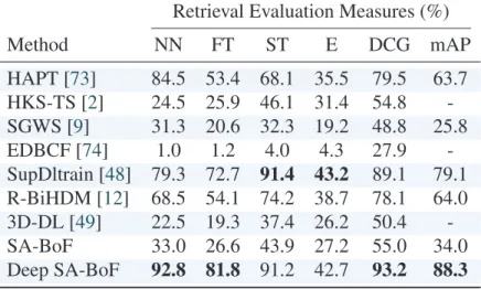
each pair of 3D shapes. The ranked list for each query shape is a set of other shapes in the dataset ranked from best to worst according to their computed distance from the query shape. In order to assess the retrieval performance several standard evaluation metrics are usually used including the precision-recall curve, nearest neighbor (NN), first-tier (FT), second-tier (ST), E-measure (E), discounted cumulative gain (DCG), and mean average precision (mAP). The definition of these evaluation measures are provided in Subsection1.5.5.
1.2.2 Shape Classification
Shape classification is all about labeling shapes in a dataset and organizing them into a known number of classes so they can be found quickly and efficiently, and the goal is to assign new shapes to one of these classes. In supervised learning tasks, the available dataZ for classification is usually split into two disjoint subsets: the training set Ztrain for learning, and the test set Ztest
for testing. The training and test sets are usually selected by randomly sampling a set of training instances from Z for learning and using the rest of instances for testing. The performance of a classifier is then assessed by applying it to test data with known target values and comparing the predicted values with the known values.
1.3
Objectives
In this thesis, we propose multi-level feature learning approaches using spectral graph wavelets, bag-of-features and deep learning models. The objective is to obtain high discriminative 3D shape descriptors in order to outperform the state-of-the-art methods that are used for either 3D shape retrieval and classification or both. Most of existing approaches are failed when it comes to dealing with recent challenging benchmarks. However, the proposed approaches show better performance in dealing with challenging datasets comparing to the state-of-the-art methods. The key factor that contributes to the success of our 3D shape descriptors is the benefit from deep learning which is used in the last stage of our feature learning frameworks to extract the most discriminative features. More specifically, we use deep auto-encoder to extract high-level features that are used to design a deep shape-aware descriptor on which retrieval test is performed. We also introduces a deep
convolutional shape-aware (Deep-CSA) learning framework for 3D shape classification using a pre-trained convolutional neural network. The aim is to beat the approaches based on hand-crafted descriptors and those obtained by shallow models.
1.4
Literature Review
In recent years, numerous schemes have been proposed to construct shape descriptors in an effort to capture the more discriminative geometric information in a 3D shape [5–13]. Inspired by the success of some descriptors in image retrieval, some works introduced 3D shape descriptor such as SIFT-based [36], Mesh-HOG [37], covariance descriptor [38]. Nevertheless, the overwhelm-ing majority of these works use spectral descriptors, which represent a shape usoverwhelm-ing a concise and compact signature. A comprehensive overview on the available spectral descriptors can be found in [39,40]. These shape representations may be broadly categorized into local and global descriptors. Local descriptors are defined on each point of the shape. Examples of local descrip-tors include the global point signature [5], heat kernel signature (HKS) [6], scale-invariant heat kernel signature (SIHKS) [7], wave kernel signature (WKS) [8], improved wave kernel signature (IWKS) [41], and spectral graph wavelet signature (SGWS) [9].
Global descriptors, on the other hand, are defined on the entire shape. One of the simplest global descriptors is Shape-DNA [42], which is defined as a truncated sequence of the LBO eigen-values arranged in increasing order of magnitude. Gaoet al.[43] introduced compact Shape-DNA (cShape-DNA) as a variant of Shape-DNA, which is an isometry-invariant signature obtained by applying the discrete Fourier transform to the area-normalized eigenvalues of the LBO. Chaud-hariet al. [11] introduced a new version of the GPS signature by setting the LBO eigenfunctions to unity. Yeet al. [12] proposed a global descriptor for nonrigid shape retrieval using a reduced biharmonic distance matrix. A graph-theoretic approach has been introduced in [44] for 3D shape classification using graph regularized sparse coding together with the biharmonic distance map. Unlike the above methods, SD-GDM [45] proposed to compute a singular value decomposition as spectrum of the geodesic distance matrix. However, compared to other spectral descriptors developed based upon the eigensystem (eigenvalues and/or eigenfunctions) of LBO as spectrum, SD-GDM relies on all-pairs geodesic distances, which are computationally prohibitive to obtain even with the latest advances in fast geodesic distance computation [46].
On the other hand, the bag-of-features (BoF) model, which has shown significant levels of per-formance in text and image retrieval, is also commonly used to construct global descriptors by aggregating the local ones. In its simplest form, the BoF model quantizes each local descriptor to its nearest cluster center using K-means clustering and then encodes each shape as a histogram over cluster centers by counting the number of assignments per cluster. These cluster centers form
a codebook whose elements are often referred to as codewords. Although the BoF paradigm has been shown to provide significant levels of performance, it does not, however, take into consid-eration the spatial relations between features, which may have an adverse effect not only on its descriptive ability but also on its discriminative power. To sidestep this issue, various solutions have been proposed including the spatially-sensitive bags-of-features (SS-BoF) [47], supervised learning of BoF shape descriptors using sparse coding [48], and geodesic-aware bags-of-features (GA-BoF) [49]. The SS-BoF, which is defined in terms of the heat kernel, can be represented by a square matrix whose elements represent the frequency of appearance of nearby codewords in the vocabulary. Similarly, the GA-BoF matrix is obtained by replacing the heat kernel in the SS-BoF with a geodesic exponential kernel.
Although the geodesic distance has proven to be effective in geometry processing due in large part to its isometry invariance property, it suffers, however, from several practical issues compared to the (squared) biharmonic distance [35]. While the geodesic distance is sensitive to topological noise and not globally shape-aware, the biharmonic distance is not only robust to noise and small topological changes, but also globally shape-aware and smooth. Our work builds upon the BoF framework to design a discriminative, shape-aware representation for 3D object classification and retrieval using the biharmonic distance in conjunction with deep neural networks [50].
Another issue with BoF model is that the codebook is usually constructed in an unsupervised manner using clustering, agnostic to the last step of the process which involves in pooling of the local descriptors into a BoF. To tackle this issue, Litmanet al.[48] proposed to replace clustering with a dictionary (codebook) learning approach coupled with sparse coding as a feature coding method. As a result, their learned BoFs have obtained in a supervised manner, being aware of feature pooling which is the last stage of BoF paradigm.
The recent trend in 3D shape analysis is to use deep learning models to learn high-level features of 3D shapes. Deep learning, which involves training neural networks on lots of data and then hav-ing them make predictions about new data, has been makhav-ing big waves over the past several years due largely to its great success in computer vision, natural language processing and speech under-standing. Deep learning models have recently been applied to 3D shape analysis to learn high-level features from 3D shapes. Wuet al.[18] proposed a deep learning framework for volumetric shapes via a convolutional deep belief network by representing a 3D shape as a probabilistic distribution of binary variables on a 3D voxel grid. Brock et al. [51] proposed a voxel-based approach to 3D object classification using variational autoencoders and deep convolutional neural networks, achieving improved classification performance on the ModelNet benchmark. Sedaghatet al.[52] showed that forcing the convolutional neural network to produce the correct orientation during training yields improved classification accuracy. The key challenge with volumetric representa-tions is how to deal with the additional computational complexity resulting from the voxelization
resolution of 3D shapes. Zhu et al. [20] introduced a a view-based technique by projecting 3D shapes into 2D images and then using an auto-encoder for feature learning. Suet al.[34] presented a convolutional neural network architecture that combines information from multiple views of a 3D shape into a single and compact shape descriptor. Qi et al. [19] proposed a multiresolution filtering strategy in order to improve the performance of multi-view convolutional neural networks on 3D shape classification. Kanezakiet al.[53] introduced RotationNet, a CNN-based framework that uses a set of multi-view images of a 3D object as input for 3D object classification and pose estimation. View-based methods tend to suffer from a relatively long running time due primar-ily to analyzing a large amount of redundant data provided by multi-view images. Also, a major drawback of view-based methods is their sensitivity to consistent model orientations, resulting in lower performance. Moreover, it is almost impossible in many real-world applications to set up multiple cameras in order to project all required views. Fanget al.[54] introduced a deep learning framework in which the heat kernel signature is fed to deep neural networks with target values in a bid to obtain a 3D deep shape descriptor that demonstrated good performance in 3D shape retrieval. Inspired by the Shape Google framework for 3D shape retrieval [47], Buet al.[49] in-troduced a deep learning based approach (3D-DL) for 3D shape classification and retrieval. The 3D-DL framework uses a 2D global shape descriptor, which is represented by a full matrix defined in terms of the geodesic distance and eigenfunctions of the LBO. The geodesic distance, however, has some major limitations, the most serious of which are the sensitivity to topological noise and the lack of shape-awareness [35]. More recently, Bu et al. [55] presented a multi-modal feature learning approach to 3D shape recognition using CNNs and convolutional deep belief networks. This hybrid approach combines both view-based and geometry-based feature learning in an effort to learn a more discriminative shape descriptor by fusing different modalities. Bai et al.[56] in-troduced a real-time 3D shape search engine based on the projective images of 3D shapes. Xieet al.[57] proposed a multi-metric deep neural network for 3D shape retrieval by learning non-linear distance metrics from multiple types of shape features, and by enforcing the outputs of differ-ent features to be as complemdiffer-entary as possible via the Hilbert-Schmid independence criterion. Tabiaet al.[58] proposed a 3D shape retrieval framework using queries of different modalities in-cluding 3D models, images and sketches. The different features extracted from different modalities are embedded into a common space using a CNN model. Chenet al.[59] introduced a multimodal learning approach to view-based 3D object classification that three modalities of image features including SIFT descriptor, Outline Fourier transform descriptor,and Zernike Moments descriptor are combined using a support vector machine. A comprehensive review of deep learning advances in 3D shape recognition can be found in [60].
1.5
Background
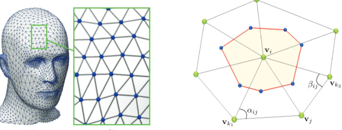
A 3D shape is usually modeled as a triangle meshMwhose vertices are sampled from a Rieman-nian manifold. A triangle meshMmay be defined as a graphG = (V,E)orG = (V,T), where
V ={v1, . . . ,vm}is the set of vertices,E ={eij}is the set of edges, andT ={t1, . . . ,tg}is the set of triangles. Each edgeeij = [vi,vj]connects a pair of vertices{vi,vj}. Two distinct vertices
vi,vj ∈ Vare adjacent (denoted byvi ∼vj or simplyi∼j) if they are connected by an edge, i.e.
eij ∈ E.
1.5.1 Laplace-Beltrami Operator
Given a compact Riemannian manifoldM, the spaceL2(M)of all smooth, square-integrable func-tions on M is a Hilbert space endowed with inner product f1, f2 = Mf1(x)f2(x)da(x), for all f1, f2 ∈ L2(M), where da(x) (or simply dx) denotes the measure from the area element of a Riemannian metric on M. Given a twice-differentiable, real-valued function f : M → R, the Laplace-Beltrami operator (LBO) is defined as ΔMf = −div(∇Mf), where ∇Mf is the intrin-sic gradient vector field and div is the divergence operator [14]. The LBO is a linear, positive semi-definite operator acting on the space of real-valued functions defined onM, and it is a gener-alization of the Laplace operator to non-Euclidean spaces.
Discretization. A real-valued functionf : V → Rdefined on the mesh vertex set may be rep-resented as an m-dimensional vector f = (f(i)) ∈ Rm, where the ith component f(i) denotes the function value at the ith vertex inV. Using a mixed finite element/finite volume method on triangle meshes [61], the value ofΔMf at a vertexvi (or simplyi) can be approximated using the cotangent weight scheme as follows:
ΔMf(i)≈ 1 ai j∼i cotαij + cotβij 2 f(i)−f(j), (1.1)
where αij and βij are the angles ∠(vivk1vj) and ∠(vivk2vj) of two faces tα = {vi,vj,vk1} and tβ = {v
i,vj,vk2} that are adjacent to the edge [i, j], andai is the area of the Voronoi cell (shaded polygon) at vertexi, as shown in Figure1.1. It should be noted that the cotangent weight scheme is numerically consistent and preserves several important properties of the continuous LBO, including symmetry and positive semi-definiteness.
Spectral analysis. The m×m matrix associated to the discrete approximation of the LBO is given byL=D−1E, whereD= diag(di)is a positive definite diagonal matrix (mass matrix), and
(a) (b)
1
Figure 1.1: Triangular mesh representation (left); Cotangent scheme angles (right).
di is the area of the Voronoi cell at vertexi, and the weightscij are given by
cij = ⎧ ⎨ ⎩ cotαij + cotβij 2 ifi∼j 0 o.w. (1.2)
whereαij andβij are the opposite angles of two triangles that are adjacent to the edge[i, j]. The eigenvalues and eigenvectors of L can be found by solving the generalized eigenvalue problem Eϕ = λDϕ using for instance the Arnoldi method of ARPACK1, where λ are the eigenvalues and ϕ are the unknown associated eigenfunctions (i.e. eigenvectors which can be thought of as functions on the mesh vertices). We may sort the eigenvalues in ascending order as
0 =λ1 < λ2 ≤ · · · ≤λm with associated orthonormal eigenfunctionsϕ1,ϕ2, . . . ,ϕm, where the orthogonality of the eigenfunctions is defined in terms of theD-inner product, i.e.
ϕk,ϕD = m
i=1
diϕk(i)ϕ(i) = δk, ∀k, = 1, . . . , m. (1.3)
We may rewrite the generalized eigenvalue problem in matrix form asEΦ=DΦΛ, whereΛis an
m×mdiagonal matrix with theλon the diagonal, andΦis anm×morthogonal matrix whose
-th column is the unit-norm eigenvectorϕ. It should be noted that since the first eigenvalueλ1is zero, its associated eigenvectorϕ1 is anm-dimensional constant vector given by
ϕ1 = 1 √ a, 1 √ a, . . . , 1 √ a , (1.4)
wherea=area(M)is the total area of the mesh.
1ARPACK (ARnoldi PACKage) is a MATLAB library for computing the eigenvalues and eigenvectors of large
1.5.2 Spectral Shape Signatures
In recent years, a great deal of 3D shape descriptors has been proposed using the spectral ana-lysis (based on eigensystem i.e. eigenvalues and/or eigenfunctions) of the LBO such as Shape-DNA [42], global point signature [5], heat kernel signature (HKS) [6], scale-invariant heat kernel signature (SIHKS) [7], wave kernel signature (WKS) [8]. It is important to point out that all of these 3D shape signatures are local descriptors, except Shape-DNA which is a global descriptor. What follows is a terse review on these spectral shape signatures.
Shape-DNA. It is one of the early proposed 3D shape signatures which is a normalized sequence of the first eigenvalues of the LBO. The simple representation (a vector of numbers) and scale invariance are the main advantages of Shape-DNA. Despite its simplicity, the shapeDNA yet has a comparable performance in 3D shape retrieval. However, the Shape-DNA cannot be used for local or partial shape analysis as it is a global descriptor. The Eigenvalue Descriptor(EVD) [62], on the other hand, is a sequence of the eigenvalues of the geodesic distance matrix. Both Shape-DNA and EVD can be normalized by the second eigenvalue.
Global Point Signature. The global point signature (GPS) [5] at a surface point is a vector of scaled eigenfunctions of the LBO. The GPS is a global feature in the sense that it cannot be used for partial shape matching. It is defined in terms of the eigenvalues and eigenfunctions ofΔM as follows: GPS(x) = ϕ2(x) √ λ2 ,ϕ√3(x) λ3 , . . . ,ϕ√i(x) λi , . . . (1.5) GPS is invariant under isometric deformations of the shape, but it suffers for the problem of eigen-functions switching whenever the associated eigenvalues are close to each other.
Heat Kernel Signature. The heat kernelpt(x, y)is an essential solution to the heat equation [63] at pointxat timetwith initial distributionu0(x) = δ(x−y)at pointy ∈ M, and it is defined in
terms of the eigenvalues and eigenfunctions ofΔMas follows: pt(x, y) = ∞ i=1 e−λitϕ i(x)ϕi(y) (1.6)
Intuitively, pt(x, y)describes the amount of heat that is propagated or transferred from pointxto point y in timet. In the same spirit, pt(x, x)describes the amount of heat that remains at point
xafter time t. For each pointx ∈ M, the Heat Kernel Signature (HKS) [6] is represented in the discrete temporal domain by an-dimensional feature vector
HKS(x) = (pt1(x, x),pt2(x, x), . . . ,ptn(x, x)) (1.7)
Scale Invariant Heat Kernel Signature. Let M and M be a shape and its uniformly scaled version by a factor ofa, respectively. Denote bypατ(x, y)the heat kernel with scale logarithmically
sampled using some basis α at each pointx. Thus, the heat kernel of the scaled shape becomes
p(τ) =a−2p(τ+ 2 log
αa). In order to remove the dependence on the multiplicative constanta−2, the logarithm of the signal is taken and then differentiated with respect to the scale variable [7]:
d dτ logp
(τ) = d
dτ(−2 loga+ logp(τ + 2 logαa)
= d dτp(τ + 2 logαa) p(τ + 2 logαa) · (1.8) Letp = dτdp(τ) p(τ) =
−i≥0λiατlogαe−λiατϕ2i(x)
−i≥0e−λiατϕ2i(x) then a new function
˜
p which transforms p˜(τ) = ˜
p(τ+ 2 logαa)as a result of scaling is obtained. The Fourier transform ofp˜and its absolute value
are given by
F p˜(ω) = ˜H(ω) = ˜H(ω)e−jω2 logαa
|H˜(ω)|=|H˜(ω)|. (1.9)
Thus, the Scale-Invariant Heat Kernel Signature (SIHKS) is defined as SIHKS(x) = |H˜(ω1)|,|H˜(ω2)|, . . . ,|H˜(ω n)| . (1.10)
Wave Kernel Signature. The basic idea of the Wave Kernel Signature (WKS) [8] is to describe a point x ∈ M by the average probabilities of quantum particles of different energy levels to be measured inx. Assume a quantum particle with unknown position is on the surface. Then the wave function of the particle is the Schrödinger equation solution, which can expressed in the spectral domain as ψE(x, t) = ∞ k=1 eiλktϕ k(x)fE(λk) (1.11)
whereE denotes the energy of the particle at timet = 0andfE its initial distribution.
Since|ψE(x, t)|2 is the probability to measure the particle at a pointxat time t, it follows that the average probability (over time) to measure a particle inxis given by
PE(x) = lim T→∞ 1 T T 0 | ψE(x, t)|2 = ∞ k=1 ϕk(x)2fE(λk)2 (1.12) LetE1, E2, . . . , En benlog-normal energy distributions. Then, each pointxon the surfaceMis associated with a wave kernel signature, which can represented by an-dimensional feature vector of average probabilities as follows:
whereei = logEi is the logarithmic energy scale. The WKS represents the average probability of measuring a quantum particle at a specific surface point. Unlike the HKS, the WKS separates influences of different frequencies, treating all frequencies equally. In other words, HKS uses low-pass filters, while WKS uses band-pass filters.
1.5.3 Deep Auto-Encoders
An auto-encoder is a neural network that learns to reproduce its input as its output. It is an un-supervised learning algorithm that learns features from unlabeled data using backpropagation via stochastic gradient descent, and has typically an input layer representing the original data, one hid-den layer and an output layer. An auto-encoder is comprised of an encoder and a decoder, as shown in Figure1.2. The encoder, denoted byfθ, maps an input vectorx∈Rdto a hidden representation (referred to as code, activations or features)a∈Rr via a deterministic mapping
a=fθ(x) =σ(Wx+b), (1.14)
parameterized by θ = {W,b}, where W ∈ Rr×d and b ∈ Rd are the encoder weight matrix and bias vector, andσ is a nonlinear element-wise activation function such as the logistic sigmoid or hyperbolic tangent. The decoder, denoted by gθ, maps back the hidden representation hto a
reconstructionxˆof the original inputxvia a reverse mapping
ˆ
x=gθ(a) =σ(Wa+b), (1.15)
parameterized byθ = {W,b}, whereW ∈ Rd×r andb ∈ Rd are the decoder weight matrix and bias vector, respectively. The encoding and decoding weight matricesWandW are usually constrained to be of the form W = W, which are referred to as tied weights. Assuming the tied weights case for simplicity, the parameters{W,b,b}of the network are often optimized by minimizing the following squared error cost function
L(W,b,b) = 1 2 N i=1 xi−xˆi22, (1.16)
where N is the number of samples in the training set, xi is the ith input sample and xˆi is its reconstruction. To penalize large weight coefficients in an effort to avoid over-fitting the training data, the following objective function is minimized instead
L(W,b,b) = 1 2 N i=1 xi−xˆi22+ λ 2W 2 F, (1.17)
whereλis a regularization parameter that determines the relative importance of the sum-of-squares error term and the weight decay term. This parameter should typically be quite small. Note that the features learned from the training data are encapsulated inW.
Encoder
Decoder
Input layer Output layer Hidden layer
Figure 1.2: Auto-encoder architecture.
An auto-encoder with multiple hidden layers is referred to as a stacked or deep auto-encoder. A stacked auto-encoder is a deep neural network consisting of multiple layers of stacked encoders from several auto-encoders. This stacked network is pre-trained layer by layer in a unsupervised fashion, where the output from the encoder of the first auto-encoder is the input of the second encoder, the output from the encoder of the second encoder is the input to the third auto-encoder, and so on. In other words, the hidden layer of the-th auto-encoder acts as an input layer to the (+ 1)-th auto-encoder. More formally, the encoding and decoding stages of anL-layer deep auto-encoder having parametersΘ ={Θ : = 1,2, ..., L}, withΘ ={W,W,b,b}, can be formulated as follows:
a =σ(Wa−1+b)
ˆ
a−1 =σ(Wa+b),
(1.18)
whereWandb(resp. Wandb) are the encoder (resp. decoder) weight matrix and bias vector of the-th auto-encoder,a0 = xandˆa0 = ˆx. After pre-training, the entire stacked auto-encoder
can be trained using backpropagation to fine-tune all the parameters of the network. 1.5.4 Convolutional Neural Networks
A Convolutional Neural Network (CNN) is a deep architecture inspired by the way humans process visual information [21]. It makes use of feedforward artificial neural networks in which individual neurons are tiled in such a way that they respond to overlapping regions in the visual field. CNNs are comprised of multiple layers that can be categorized into three types: convolutional, subsam-pling and fully-connected. A convolutional layer consists of a rectangular grid of neurons, and applies a set of filters that process small local parts of the input where these filters are replicated along the whole input space. Each neuron takes inputs from a rectangular section of the previous layer; the weights for this rectangular section are the same for each neuron in the convolutional layer. Thus, the convolutional layer is just an image convolution of the previous layer, where the weights specify the convolution filter. A subsampling (pooling) layer takes small rectangular
blocks from the convolutional layer and subsamples it with average or max pooling to produce a single output from that block. This adds translation invariance and tolerance to minor differences of positions of objects parts. Higher layers use more broad filters that work on lower resolution inputs to process more complex parts of the input. Similar to a feedforward neural network, a fully connected layer takes all neurons in the previous layer and connects them to each of its neurons. CNNs can be trained using standard backpropagation. The CNN architecture shown in Figure1.3
is composed of 5 layers: two convolutional layers (C1 and C2), two subsampling layers (S1 and S2) and one fully connected layer. For classification tasks, an output layer is added after the fully connected layer.
Figure 1.3: Basic architectures of a CNN.
More specifically, the input to a convolutional layer is anm ×m ×r image where m is the height and width of the image andris the number of channels, e.g. an RGB image hasr = 3. The convolutional layer will havek filters (or kernels) of sizen×n×q wheren is smaller than the dimension of the image andq can either be the same as the number of channelsr or smaller and may vary for each kernel. The size of the filters gives rise to the locally connected structure which are each convolved with the image to producekfeature maps of sizem−n+ 1. Each map is then subsampled typically with average or max pooling overp×pcontiguous regions, wherepranges between 2 for small images and is usually not more than 5 for larger inputs. Either before or after the subsampling layer an additive bias and a sigmoidal nonlinear activation function is applied to each feature map. After the convolutional layers there may be any number of fully connected layers. The densely connected layers are identical to the layers in a standard multilayer neural network.
1.5.5 Performance Evaluation Measures
In this section, we discuss in detail the measures that are commonly used to evaluate the perfor-mance of nonrigid 3D shape retrieval and classification. We first discuss the evaluation metrics for
3D shape retrieval which are precision-recall curve, nearest neighbor (NN), first-tier (FT), second-tier (ST), E-measure (E), discounted cumulative gain (DCG), and mean average precision (mAP).
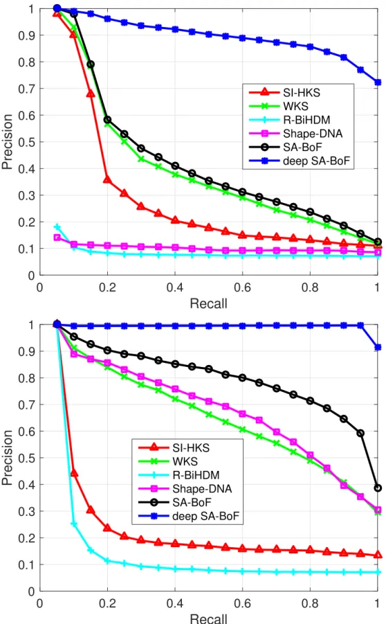
Precision-Recall Graph. A precision-recall graph demonstrates the behavior of precision and
recall in a ranked list of retrieved shapes. Assume the category that query shape belongs to hasC
members including query shape itself and we retrieve topK matches. Recall is the ratio of shapes
in query’s category that are retrieved among topK matches, while precision is the ratio of topK
matches that belong to the query’s category. The perfect retrieval results must give the highest
precision (i.e. 100%) for all recall which may be illustrated by a horizonal line at the top of the
plot (i.e. precision = 1.0). Hence, a precision-recall graph that is shifted upwards and to the right
indicates superior performance.
Nearest Neighbor.The NN metric is the percentage of the closest matches that belong to the same
category of query’s, i.e. for each shape in the dataset, the second best result (obviously, the best result is a match with query itself) is verified wether it is a member of the same category that the
query shape belongs to. The ideal score is definitely100%and the higher score indicates the better
results.
First-Tier and Second-Tier. The FT metric is the percentage of the shapes belong to the query’s
category that are retrieved in the topC−1matches, where query’s category hasCmembers. The
recall for ST metric is twice as big as for ST metric, i.e. the percentage of the shapes belong to
the query’s category that are retrieved in the top 2(C − 1)matches. Obviously, the ideal score
for both metrics are100%and the higher values represents better results, while the higher score is
more likely to appear for ST metric as the members of query’s category have more chance to be retrieved among top matches.
E-measures. This metric is obtained when precision and recall are calculated for the first 32
matches in the ranked list (i.e. K = 32). The E-measure is defined as:
E = 1 2
P +
1
R
, (1.19)
whereP andRare precision and recall, respectively. The maximum value for this metric is1.0(or
equivalently100%in terms of percentages) and the higher scores indicates the better results.
Discounted Cumulative Gain. This metric weighs relevant results on the top of ranked list more
than the relevant results at the bottom of the ranked list. The intuition is that the query results of the first pages are more of interest to a user of a search engine than those of the later pages. This
metric have scores ranging from 0% to 100% and the higher score indicates the better retrieval
Mean Average Precision. The mAP metric is defined as:
mAP =X
K
P(K)R(K), (1.20)
where precision and recall are calculated for all values ofK. Intuitively, mAP is considered the
area below the precision-recall graph. A perfect retrieval algorithm has mAP= 100%and a higher
value indicates better results.
Confusion Matrix. The performance of a classifier is usually evaluated via the confusion matrix,
which displays the number of correct and incorrect predictions made by the classifier compared with the actual classifications in the test set. The confusion matrix shows how the predictions are made by the model. The rows correspond to the actual (true) class of the data (i.e., the labels in the data), while the columns correspond to the predicted class (i.e., predictions made by the model). When an instance is classified, it is the same as making a prediction that the instance is correctly classified. The elements of the confusion matrix for binary (two-class) classification problem are
• TP (true positives) is the number of positive instances correctly classified
• FP (false positives) is the number of negative instances incorrectly classified as positive
• FN (false negatives) is the number of positive instances incorrectly classified as negative
• TN (true negatives) is the number of negative instances correctly classified
The value of each element in the confusion matrix is the number of predictions made with the class corresponding to the column for instances (examples) with the correct value as represented by the row. Thus, the diagonal elements show the number of correct classifications made for each class, and the off-diagonal elements show the errors made.
Classification Accuracy. Another intuitively appealing measure is the classification accuracy,
which is a summary statistic that can be easily computed from the confusion matrix as the total number of correctly classified instances (i.e. diagonal elements of confusion matrix) divided by the total number of test instances. Alternatively, the accuracy of a classification model on a test set may be defined as follows
Accuracy = Number of correct classifications
Total number of test cases
= |z : z∈ Ztest ∧ yˆ(z) = y(z)| |z : z∈ Ztest| ,
(1.21)
where y(z) is the actual (true) label of z, and yˆ(z) is the label predicted by the classification
algorithm. A correct classification means that the learned model predicts the same class as the original class of the test case.
1.6
Overview and Contributions
The organization of this thesis is as follows
• Chapter 1 begins with the basic concepts which we refer to throughout the thesis, gives our motivations and goals for this research, followed by the problem statement, the objective of this study, a literature review, and a brief discussion of background context to the develop-ment of our 3D shape analysis framework.
• In Chapter 2, we introduce a multi-level feature learning framework for 3D shape retrieval using using spectral graph wavelets, bag-of-features, and deep learning [64]. The proposed 3D shape retrieval approach is evaluated on three standard 3D shape datasets through exten-sive experiments, and the results show compelling superiority of our approach over state-of-the-art methods.
• In Chapter 3, we propose a deep learning approach to 3D shape retrieval using a multi-level feature learning paradigm [65]. Low-level features are first extracted from a 3D shape us-ing spectral graph wavelets. Then, mid-level features are generated via the bag-of-features model by employing locality-constrained linear coding as a feature coding method, in con-junction with the biharmonic distance and intrinsic spatial pyramid matching in a bid to ef-fectively measure the spatial relationship between each pair of the bag-of-feature descriptors. Finally, high-level shape features are learned by applying a deep auto-encoder on mid-level features. Extensive experiments on three standard 3D shape datasets demonstrate the much better performance of the proposed framework in comparison with state-of-the-art methods, and also a framework developed based on a shallow model.
• In Chapter 4, we present a deep learning approach to 3D shape classification using convo-lutional neural networks [66] using the bag-of-features model in conjunction with intrinsic spatial pyramid matching that leverages the spatial relationship between features. These 2D images are then fed into a pre-trained convolutional neural network to learn deep convolu-tional shape-aware descriptors from the penultimate fully-connected layer of the network. Finally, a multiclass support vector machine classifier is trained on the deep descriptors, and the classification accuracy is subsequently computed. The effectiveness of our approach is demonstrated on three standard 3D shape benchmarks, yielding higher classification accu-racy rates compared to existing methods.
• Chapter 5 presents a summary of the contributions of this proposal, limitations, and outlines several directions for future research in this area of study.
C
HAPTER
2
Deep Shape-Aware Descriptor for 3D Object
Retrieval
Deep learning has become a pervasive and wide reaching technology, growing at a breathtaking rate and achieving remarkable results on a variety of fields, including computer vision, image and speech recognition, and natural language processing. In this chapter, we propose a deep learning approach for 3D shape retrieval using a multi-level feature learning methodology. We first ex-tract low-level features or local descriptors from a 3D shape using spectral graph wavelets. Then, we construct mid-level features from these local descriptors via the bag-of-features paradigm by employing locality-constrained linear coding as a feature coding method, together with the bihar-monic distance as a measure of the spatial relationship between each pair of bag-of-feature de-scriptors. Finally, high-level shape features are learned via a deep auto-encoder, resulting in a deep shape-aware descriptor that is compact, geometrically informative and efficient to compute. The proposed 3D shape retrieval approach is evaluated on SHREC-2014 and SHREC-2015 datasets through extensive experiments, and the results show compelling superiority of our approach over state-of-the-art methods.
2.1
Introduction
In recent years, spectral geometry has been key in the development of efficient algorithms for nonrigid 3D shape retrieval, achieving state-of-the-art performance on the latest shape retrieval contests [1,2]. Most spectral-geometric methods make use of a shape signature or descriptor, which is a concise and compact representation of a shape, aimed at facilitating the retrieval task.
These shape representations may be categorized into local and global descriptors. Local descrip-tors (also known as point signatures) are usually defined on each point of the shape, while global descriptors are defined on the entire 3D shape. Examples of local descriptors include the global point signature (GPS) [5], heat kernel signature (HKS) [6], scale-invariant heat kernel signature (SI-HKS) [7], wave kernel signature (WKS) [8], and spectral graph wavelet signature (SGWS) [9]. On the other hand, many global descriptors can be constructed from point signatures by integrating over the entire shape. One of the simplest global descriptors is Shape-DNA [42], which is defined as a truncated sequence of the Laplace-Beltrami operator (LBO) eigenvalues arranged in increas-ing order of magnitude. Chaudhari et al. [11] presented a slightly modified version of the GPS signature by setting the LBO eigenfunctions to unity. Ye et al.[12] proposed a global descriptor for nonrigid shape retrieval using a reduced biharmonic distance matrix.
Another type of commonly-used global descriptors are constructed by aggregating the local de-scriptors using the bag-of-features (BoF) paradigm. In its simplest form, the BoF model quantizes each local descriptor to its nearest cluster center using K-means clustering and then encodes each shape as a histogram over cluster centers by counting the number of assignments per cluster. These cluster centers form a codebook whose elements are often referred to as codewords. Although the BoF paradigm has been shown to provide significant levels of performance, it does not, however, take into consideration the spatial relations between features, which may have an adverse effect not only on its descriptive ability but also on its discriminative power. To account for the spatial rela-tions between features, Bronsteinet al.[47] introduced a generalization of a bag of features, called spatially sensitive bags of features (SS-BoF). Litmanet al.[48] proposed a supervised approach to learn BoF shape descriptors using sparse coding.
Deep learning models have been recently used in 3D shape analysis to learn high-level features of 3D shapes. The most popular deep learning models that have been successfully applied to image data include deep convolutional neural networks, deep auto-encoders, deep belief networks and deep Boltzmann machines [21–33]. Although a few studies [67,68] proposed to apply deep models directly to 3D data, many frameworks first represent a 3D shape by a 2D image and then apply a deep architecture for feature learning. For this purpose, the more conventional way is to capture the object by a set of 2D images from different views. Zhu et al.[20] introduced a a view-based technique by projecting 3D shapes into 2D images and then using an auto-encoder for feature learning. A major drawback of view-based methods is their sensitivity to consistent model orientations, resulting in lower performance [3].
Another route to represent a 3D shape as a 2D image is to capture geometric and topological properties of the model and then demonstrate it as a 2D signal. These graphical informative rep-resentation are usually obtained by using global shape descriptors. For instance, Bu et al. [49] presented a deep learning framework (3D-DL) for 3D shape classification and retrieval. 3D-DL
extracts high-level features by applying deep belief networks (DBNs) on 2D global descriptor ob-tained by the geodesic distance and eigenfunctions of the LBO. The main issue with geodesic distance lies in its sensitivity to topological noise not to mention, it often fails to capture the global properties of a shape compared to the (squared) biharmonic distance [35].
In this chapter, we adopt a similar strategy as [49] in the sense that we employ deep learn-ing to 3D shape retrieval, but our approach differs in the way our deep shape descriptor is com-puted. More specifically, we introduce a multi-level feature learning approach using spectral graph wavelets, bag-of-features and deep auto-encoders. In particular, we use the spectral graph wavelet signature as a local descriptor due is its ability to capture different details provided at different levels from low to high frequencies. We also use locality-constrained linear coding (LLC) as a feature coding scheme in the BoF model due largely to the lower quantization error of LLC as well as its codewords locality properly. In addition, we employ the biharmonic distance to measure the spatial relationship between the LLC codes. Unlike the geodesic distance which is not globally shape-aware, the biharmonic distance is shape-ware, isometry invariant, computationally efficient, robust to various shape deformations, and possesses good discriminative capabilities [12,35]. The main contributions of this chapter may be summarized as follows:
1. We present low-level shape descriptors using spectral graph wavelets.
2. We construct mid-level features using the BoF model in which we employ LLC as a feature coding scheme. We then measure the spatial relationship between the LLC codes via the biharmonic distance in order to generate shape-aware bag-of-features.
3. We employ a deep auto-encoder to learn high-level features that are used to design a deep shape-aware descriptor for 3D shape retrieval tasks.
The rest of this chapter is structured as follows. In Section2.2, we introduce a multi-level 3D shape feature learning framework using deep learning, and we discuss in detail its major compo-nents as well as its algorithmic steps. Section2.3presents the experimental results and Section2.4
concludes the chapter.
2.2
Proposed Framework
In this section, we describe the main components and algorithmic steps of the proposed multi-level feature learning framework. The approach consists of three major components: low-level features, mid-level features and high-level features, as illustrated in Figure 2.1. In the low-level features construction, we use spectral graph wavelets to generate local descriptors for each 3D shape in the dataset. In the mid-level features step, we used the BoF model in conjunction with the biharmonic
distance to construct shape-aware global descriptors. In the third step, high-level shape features are learned using deep auto-encoders.
Dataset Low-Level Descriptors Mid-Level Features
SA-BoF LLC Codebook LLC Codes SGWS High-Level Features input layer hidden layer output layer Auto-Encoder Learned Features
Figure 2.1: Main components of the proposed feature learning method: low-level features, mid-level features and high-mid-level features.
2.2.1 Low-Level Features
Wavelets are useful in describing functions at different levels of resolution. Motivated by the effectiveness of the multiresolution SGWS in 3D shape retrieval [9], we propose an improved spectral graph wavelet signature by incorporating the vertex area into the signature. For a given resolution parameterR, the improved SGWS at vertexj is ap-dimensional vector defined as
sj ={sQ(j)|Q= 1, . . . , R}, (2.1) wheresQ(j)is the shape signature at vertexj and resolution levelQ, and is given by
sQ(j) = {Wδj(tq, j)|q= 1, . . . , Q} ∪ {Sδj(j)}. (2.2) At each resolution levelQ, the signaturesQ(j)at vertexj is an(Q+ 1)-dimensional vector con-sisting of spectral graph wavelet coefficientsWδj(tq, j)given by
Wδj(tq, j) = m
=1
a2jg(tqλ)ϕ2(j), q = 1, . . . , Q (2.3) and scaling function coefficientsSδj(j)given by
Sδj(j) = m
=1
wheregandhare the spectral graph wavelet generating kernel and scaling function, respectively. The spectral graph wavelet generating kernelg acts as a band-pass filter, whilehis used as a low-pass filter to encode the low-frequency content of a function defined on the mesh vertices [9]. The wavelet scalestq (tq > tq+1) are selected to be logarithmically equispaced between maximum and
minimum scales t1 and tQ, respectively. The dimension of sj can be expressed in terms of the resolution parameterRas follows:
p= (R+ 1)(R+ 2)
2 −1. (2.5)
For example, at resolutionR = 2, the spectral graph wavelet signaturesj is a 5-dimensional vector consisting of five elements (four elements of spectral graph wavelet function coefficients and one element of scaling function coefficients).
For ap-dimensional signaturesi, we define ap×mspectral graph wavelet signature matrix as
S = (s1, . . . ,sm), wheresi is the signature at vertexi andm is the number of mesh vertices. In our implementation, we used the cubic spline wavelet and the scaling functions given by
g(x) = ⎧ ⎪ ⎪ ⎪ ⎨ ⎪ ⎪ ⎪ ⎩ x2 ifx <1 −5 + 11x−6x2+x3 if1≤x≤2 4x−2 ifx >2 (2.6) and h(x) = γexp − x 0.6λmin 4 , (2.7)
whereλmin =λmax/20andγ is set such thath(0)has the same value as the maximum value ofg. The maximum and minimum scales are set tot1 = 2/λminandtQ= 2/λmax.
2.2.2 Mid-Level Features
In the second step of the proposed approach, we compute sparse codes for the local descriptors us-ing the BoF model, which aggregates these descriptors in order to provide a simple representation that may be used to facilitate comparison between 3D shapes. We then propose new shape de-scriptors that are globally shape-ware, robust to topological noise and practical to compute. These shape-aware descriptors are defined in terms of the biharmonic distance and the sparse codes.
Bag-of-Features Model
The BoF model consists of four main steps: feature extraction and description, codebook design, feature coding and feature pooling. We model a 3D shape as a triangle meshMwithmvertices.
Feature extraction and description. In the BoF paradigm, a 3D shape M is represented as a collection of m local descriptors of the same dimension p, where the order of different feature vectors is of no importance. Local descriptors may be classified into two main categories: dense and sparse. Dense descriptors are computed at each vertex of the mesh, while sparse descriptors are computed by identifying a set of salient points using a feature detection algorithm. In our approach, we represent the shapeMby ap×mmatrixS= (s1, . . . ,sm)of spectral graph wavelet signatures, where eachp-dimensional feature vectorsi is a dense, local descriptor that encodes the local structure around thei-th vertex of the mesh.
Codebook design. We construct a codebook (also called vocabulary or dictionary) offline by applying the K-means algorithm to a representative collection of local descriptors. To this end, we used the idea of intrinsic spatial partition [69] to select representative descriptors in a way that ensures each partition of a shape participates in the codebook design procedure. We may represent the codebook by ap×k vocabulary matrixV = (v1, . . . ,vk)ofp-dimensional vectorsvi called codewords (also known as basis vectors or atoms), which are the centroids of the clusters.
Feature coding. Given a codebook, each local descriptorsimay be mapped to a codeword in the vocabulary space using feature coding techniques such hard-assignment, soft-assignment, sparse coding and locality-constrained linear coding [70], to name just a few. While sparse coding has shown promising results as a feature coding method in the BoF model [48], it uses, however, sparsity constraint and has no priorities for the closer codewords to each local descriptor over the further ones. Locality-constrained linear coding (LLC), on the other hand, employs locality con-straint to enforce codebook locality instead of sparsity. As a result, LLC yields smaller coefficients for codewords farther away fromsi. More precisely, the LLC code ui is obtained by solving the following regularized least-squares problem
ui = arg min
1ui=1
si−Vui22+λdiui22, (2.8)
wheredenotes the element-wise multiplication,di = exp(dist(si,V)/δ)measures the similarity between thei-th descriptor and all the codewords with dist(si,V) = (si−v12, . . . ,xi−vk2), andδis a parameter to adjust the weight decay speed for the locality adaptor.
It should be noted that the LLC code is not sparse in the sense of0-norm, but it is sparse in the
sense that the codes have only a few elements with significant values. In practice, an approximated LLC is employed for fast encoding by removing the regularization term (i.e. locality constraint) from (2.8) and instead using thernearest neighbors ofsias a set of codewords [70], thereby reduc-ing the computational complexity fromO(k2)toO(k+r2), wherek is the number of codewords in the vocabulary andrk.
Hence, each p-dimensional local descriptor si is encoded by a k-dimensional LLC code ui, resulting in ak×mmatrixU= (u1, . . . ,um)which we refer to as the LLC codes matrix.
Feature pooling. Each spectral graph wavelet signature is mapped to a certain codeword through the clustering process and the shape is then represented by the histogramhof the codewords, which is ak-dimensional vector given by
h=U1m = (hr)r=1,...,k (2.9)
wherehr =
m
i=1uri. That is, the histogram consists of the column-sums of the cluster assign-ment matrix U. Other feature pooling methods include average- and max-pooling. In general, a feature vector is given byh =P(U), wherePis a predefined pooling function that aggregates the information of different codewords into a single feature vector.
Shape-Aware Bag-of-Features
A major drawback of the BoF model is that it only considers the distribution of the codewords and disregards all information about the spatial relations between features, and hence the descriptive ability and discriminative power of the BoF paradigm may be negatively impacted. To circumvent this limitation, various solutions have been recently proposed including the spatially sensitive bags of features (SS-BoF) [47] and geodesic-aware bags of features (GA-BoF) [49]. The SS-BoF, which is defined in terms of the heat kernel, can be represented by a square matrix whose elements represent the frequency of appearance of nearby codewords in the vocabulary. Similarly, the GA-BoF matrix is obtained by replacing the heat kernel in the SS-GA-BoF with a geodesic exponential kernel. Although the geodesic distance has proven to be effective in tackling nonrigid 3D shape matching and retrieval [71,72] due in large part to its isometry invariance property, it suffers, however, from several disadvantages compared to the (squared) biharmonic distance [35]. While the geodesic distance is not smooth, sensitive to topological noise and not globally shape-aware, the biharmonic distance is not only robust to noise and small topological changes, but also globally shape-aware and smooth. As shown in Figure 2.2, the level sets of the biharmonic distance are much smoother than those of the geodesic distance. Notice that the source point is displayed as a small green sphere, located in the vicinity of the mouth of the 3D face model. Both distances are computed from the source point to all the remaining points of the 3D face model.
In addition to its isometry invariance, the biharmonic distance is practical to compute, and strikes a balance between nearly geodesic distances for small distances and global shape-awareness for large distances. Inspired by these nice properties, we define a shape-ware descriptor of a 3D shape as ak×kmatrixFgiven by
F=UKU, (2.10)
whereUis ak×mmatrix of LLC codes, andK= (κij)is anm×mbiharmonic distance kernel matrix whose elements are defined in terms of the eigenvalues and eigenfunctions of the LBO as
Figure 2.2: A 3D face model color-coded by the biharmonic (left) and geodesic distances (right). Darker blue regions indicate smaller distances, while darker red regions indicate larger distances. Level sets (isocontours) are displayed as white lines at equally spaced intervals of distance.
follows: κij = m =1 1 λ2(ϕ(i)−ϕ(j)) 2. (2.11)
We refer toFas a shape-aware bag-of-features (SA-BoF) matrix, which indicates the occurrence distribution of the codewords and the spatial relationships between them. Hence, for each 3D shape, the mid-level features are represented by ak×kmatrixFcontaining global descriptors. 2.2.3 High-Level Features
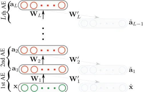
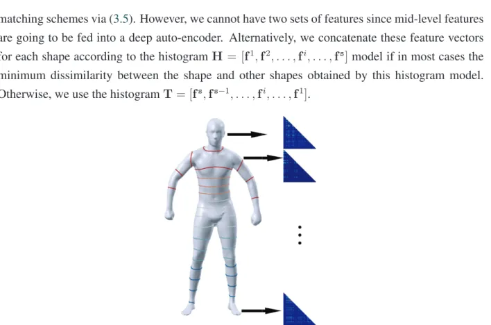
In the third step of our framework, more discriminative 3D shape descriptors are extracted using high-level features learned by performing a deep auto-encoder on the mid-level features. Unlike images, a 3D mesh cannot be fed directly into a deep learning model. To tackle this issue, we use the k ×k SA-BoF matrix (viewed as an image) For more precisely the k2-dimensional vector
x as an input to the deep auto-encoder, where x is obtained by stacking the columns of F one underneath the other. The high-level features are then extracted from the output of the last hidden layer of the deep auto-encoder, resulting in anrL-dimensional high-level feature vectoraL, which we refer to as a deep SA-BoF descriptor, whererLis the total number of neurons in the last hidden layer, as illustrated in Figure2.3.
2.2.4 Proposed Algorithm
The goal of 3D shape retrieval is to search and extract the most relevant shapes to a query object from a dataset of 3D shapes. The retrieval accuracy is usually evaluated by computing a dissimi-larity measure between pairs of 3D shapes in the dataset. A good retrieval algorithm should result in few dissimilar shapes. A commonly used dissimilarity measure for content-based retrieval is the
1st AE
{
{
{
2nd AE
th AE
Figure 2.3: Deep auto-encoder architecture. The hidden layer of the 1st auto-encoder (AE) is trained to reconstruct the input data. Then, the hidden layer of the 2nd AE is trained to reconstruct the hidden layer of the 1st AE, and so on.
As stated previously, our learning framework consists of three main components. In the first step, we represent each 3D shape in the dataset by a spectral graph wavelet signature matrix, which is a feature matrix whose columns are the local shape descriptors. More specifically, letD be a dataset of n shapes modeled by triangle meshes M1, . . . ,Mn. We represent each meshMi by ap×m spectral graph wavelet signature matrixSi, wherem is the number of mesh vertices. The spectral graph wavelet signatures are then encoded via LLC, resulting in ak ×mmatrixUi whose columns are thek-dimensional LLC codes. In the second step, thek×kSA-BoF matrixFi is computed using the