Model based forecasting for demand response strategies

(1)

Acceptée sur proposition du jury

pour l’obtention du grade de Docteur ès Sciences par

Lorenzo NESPOLI

Présentée le 7 juin 2019

Thèse N° 9415

Dr J. Van Herle, président du jury

Prof. F. Maréchal, Prof. A. E. Rizzoli, directeurs de thèse Prof. M. Merlo, rapporteur

Prof. A. Bemporad, rapporteur Prof. M. Paolone, rapporteur

à la Faculté des sciences et techniques de l’ingénieur Groupe SCI STI FM

(2)

(3)

This makes forecasting something between tremendously difficult and actually impossible, with a strong shift toward the latter as timescales get longer.”

— Andrew McAfee

“There is no way that we can predict the weather six months ahead beyond giving the seasonal average” — Stephen Hawking

(4)

(5)

Acknowledgements

The publication of this manuscript concludes a personal amazing journey which couldn’t have been possible without the trust placed in me by Roman Rudel and Davide Rivola when I firstly arrived at the ISAAC institute at SUPSI 5 years ago. To them goes my gratitude, also for giving me a lot of freedom in directing my own research through my interests.

I would like to thank François Maréchal for having been my supervisor at the EPFL, for all the insightful discussions and for directing my work towards scientifically sound results. Many thanks also to Andrea Rizzoli for guiding me through the PhD and to his group at IDSIA, especially to Matteo Salani and Marco Derboni.

My deepest thanks goes to Vasco Medici for the great support he gave me in both the nu-merous projects and publications carried out together, his endless patience in helping me to improve my coding capabilities and for going through the bleeding-eye process of correcting my bugged codes. I am very grateful to Davide Strepparava for all the technical support he gave me and for sharing his experience, without with, a lot of tasks like data gathering would have been much more painful. A special thanks to Gianluca Corbellini for being my mentor, in life more than anything else, and for sharing with me his view of the world.

It has been a pleasure to work with the people of the DESL laboratory of EPFL, in particular I would like to thank Mario Paolone and Fabrizio Sossan for the fruitful collaboration in the context of the SCCER-FURIES competence center.

I would also like to thank Pantelis Sopasakis for having kindly introduced me to decomposition techniques and for his handwritten explanations, which have been of great help, and Alberto Bemporad for providing me with information on model predictive control and background material on stochastic optimization.

My gratitude goes to the Henrik Madsen from DTU for his great course on system identifica-tion, and to the DTU Center for Electric Power and Energy for the introduction to the field of optimization in energy systems, especially the group of Pierre Pinson, Vladimir Dvorkin and Fabio Moret for the short but helpful discussions on energy communities.

Last but not least I would like to thank Carolina Carmo, Sawsa Hadi, Amin Shokri Gazafroudi, Enrica Scolari, Federico Rosato, Ruben Baetens, and many others who have shared with me part of this journey.

(6)

Finally I would like to thanks my parents for their unconditional support they gave me, Miriam for her endless caring, both my brothers Federico and Tenchi, my old date friends Fabrizio, Simone, Filippo, Alessandro and all the other friends who make me feel home every time I come back, and Giulio.

(7)

Abstract

The incremental deployment of decentralized renewable energy sources in the distribution grid is triggering a paradigm change for the power sector. This shift from a centralized struc-ture with big power plants to a decentralized scenario of distributed energy resources, such as solar and wind, calls for a more active management of the distribution grid. Conventional distribution grids were passive systems, in which the power was flowing unidirectionally from upstream to downstream. Nowadays, and increasingly in the future, the penetration of distributed generation (DG), with its stochastic nature and lack of controllability, represents a major challenge for the stability of the network, especially at the distribution level. In par-ticular, the power flow reversals produced by DG cause voltage excursions, which must be compensated. This poses an obstacle to the energy transition towards a more sustainable energy mix, which can however be mitigated by using a more active approach towards the con-trol of the distribution networks. Demand side management (DSM) offers a possible solution to the problem, allowing to actively control the balance between generation, consumption and storage, close to the local point of generation. An active energy management implies not only the capability to react promptly in case of disturbances, but also the ability to anticipate future events and take control actions accordingly. This is usually achieved through model predictive control (MPC), which requires a prediction of the future disturbances (in this case, produced and consumed energy) acting on the system.

This thesis treats challenges of distributed DSM, with a particular focus on the case of a high penetration of PV power plants. The first subject of the thesis is the evaluation of the performance of models for forecasting and control with low computational requirements, of distributed electrical batteries. The proposed methods are compared by means of closed loop deterministic and stochastic MPC performance. The second subject of the thesis is the development of model based forecasting for PV power plants, and methods to estimate these models without the use of dedicated sensors. The third subject of the thesis concerns strategies for increasing forecasting accuracy when dealing with multiple signals linked by hierarchical relations. Hierarchical forecasting methods are introduced and a distributed algorithm for reconciling base forecasters is presented. At the same time, a new methodology for generating aggregate consistent probabilistic forecasts is proposed. This method can be applied to distributed stochastic DSM, in the presence of high penetration of rooftop installed PV systems. In this case, the forecasts’ errors become mutually dependent, raising difficulties in the control problem due to the nontrivial summation of dependent random variables. The benefits of considering dependent forecasting errors over considering them as

(8)

independent and uncorrelated, are investigated. The last part of the thesis concerns models for distributed energy markets, relying on hierarchical aggregators. To be effective, DSM requires a considerable amount of flexible load and storage to be controllable. This generates the need to be able to pool and coordinate several units, in order to reach a critical mass. In a real case scenario, flexible units will have different owners, who will have different and possibly conflicting interests. In order to recruit as much flexibility as possible, it is therefore important to design incentive mechanisms that guarantee participants to benefit from their participation, while at the same time achieving a technical optimum. Since I didn’t want to include any users’ active decision nor belief in the formation of the market equilibrium price, or to model users’ willingness to pay and their marginal utilities, I chose not to consider auction mechanisms. I instead used the well known concept of Lagrangian relaxation from optimization theory, and the interpretation of Lagrangian multipliers as marginal prices, as a way to automatically identify prices for the grid’s constraints. I further avoided to model users’ utility as intended in standard auction and game theory, and replaced it with costs and users’ constraints sets. In fact, the latter can be interpreted as a binary and non differentiable utility function, and prevent us from making any assumption on users’ marginal satisfaction with respect to consumed energy. The focus is on two approaches, the first one relying on distributed control theory, while the second one generates from non-cooperative games. I show that for the class of problems of our interest, the so called sharing problems, the two formulations are deeply linked, and can thus be treated using the same decomposition techniques.

(9)

Sinossi

La progressiva adozione di fonti energetiche rinnovabili decentralizzate nella rete di dis-tribuzione sta innescando un cambiamento di paradigma per il settore energetico. Il passag-gio da una struttura centralizzata a uno scenario di produzione di energia elettrica tramite fonti distribuite, come il solare e l’eolico, richiede una gestione più attiva della rete di dis-tribuzione. Le reti di distribuzione erano considerate sistemi passivi, in cui la potenza fluisce unidirezionalmente dalla fonte di produzione al consumatore. Oggigiorno, e sempre più in futuro, la penetrazione della generazione distribuita (GD), con la sua natura stocastica e la mancanza di controllabilità, rappresenta una grande sfida per la stabilità della rete, soprattutto a livello della rete di distribuzione. In particolare, le inversioni del flusso di potenza prodotte da GD provocano escursioni di tensione, che devono essere compensate. Ciò rappresenta un ostacolo alla transizione energetica verso un mix energetico più sostenibile, che può tuttavia essere mitigato utilizzando un approccio più attivo verso il controllo delle reti di distribuzione. Il Demand Side Management (DSM) offre una possibile soluzione al problema, consentendo di controllare attivamente l’equilibrio tra generazione, consumo e stoccaggio. Una gestione energetica attiva implica non solo la capacità di reagire prontamente in caso di disturbi, ma anche la capacità di anticipare eventi futuri e intraprendere azioni di controllo di conseguenza. Questo è solitamente ottenuto attraverso modelli di controllo predittivo, che richiedono una previsione dei disturbi futuri che agiscono sul sistema. Questa tesi tratta le sfide del DSM distribuito, con particolare attenzione al caso di un’ alta penetrazione di impianti fotovoltaici. Il primo argomento della tesi è la valutazione delle performance di modelli con requisiti com-putazionali limitati per il controllo di batterie elettriche distribuite. I metodi proposti sono confrontati per mezzo delle loro prestazioni a ciclo chiuso, sia per un controllo deterministico che stocasticho. Il secondo argomento della tesi è lo sviluppo di metodi per la previsione della potenza generata da impianti fotovoltaici, basati su modelli fisici, e la stima degli stessi senza l’uso di sensori dedicati. Il terzo argomento indagato nella tesi sono strategie per au-mentare l’accuratezza della predizione della potenza e consumo elettrico in vari punti della rete di distribuzione, avendo a disposizione dati storici collegati da relazioni gerarchiche. In particolare, è presentato un metodo per calcolare in modo distribuito diverse techniche di riconciliazione per predittori gerarchci. In concomitanza, è presentata una nuova metodologia per l’aggregazione consistente delle distribuzioni di probabilità descriventi previsioni della generazione di potenza. Questo metodo può essere applicato al DSM stocastico distribuito, in presenza di elevata penetrazione di impianti fotovoltaici. In questo caso infatti, gli errori delle previsioni diventano mutualmente dipendenti, inducendo difficoltà nel problema di controllo,

(10)

dovute alla non trivialità della somma di distribuzioni di probabilità dipendenti. I vantaggi di considerare gli errori di previsione come dipendenti, sono mostrati nella tesi. L’ultima parte della tesi riguarda modelli per i mercati elettrici distribuiti, basati su aggregatori gerarchici. Per essere efficace, il DSM richiede il controllo di un gran numero di utenti. Questo genera la necessità di essere in grado di raggruppare e coordinare diversi consumatori e produtori nella rete elettica, al fine di raggiungere una massa critica. In un caso reale, le risorse di flessibilità avranno proprietari diversi, con interessi economici conflittuali. Al fine di reclutare la massima flessibilità possibile, è quindi importante progettare meccanismi di incentivazione che garantiscano ai partecipanti di beneficiare della loro partecipazione, ottenendo allo stesso tempo un optimum tecnico. Poiché non volevo delegare nessun ruolo attivo agli utenti nella determinazione del prezzo di equilibrio del mercato, né modellare la loro utilità marginale, ho scelto di non considerare meccanismi d’asta. Ho invece usato concetti di ottimizzazione e in particolare la teoria dei moltiplicatori di Lagrange per determinare il prezzo legato ai vincoli di rete in modo automatico. Ho inoltre evitato di modellare l’utilità degli agenti, come intesa nella teoria delle aste a dei giochi, sostituendola con costi e set di vincoli per gli utenti. Questi ultimi possono infatti essere considerati come funzioni di utilità binarie non differenziabili, e permettono di non fare nessun assunzione sulla soddisfazione marginale degli utenti nel consumare energia. In particolare, ho concentrato l’attenzione su due approcci diversi: il primo basato sulla teoria del controllo distribuito, il secondo basato sulla teoria dei giochi non cooperativi. Nella tesi viene dimostrato che per la classe di problemi di nostro interesse, i cosiddetti sharing problems, le due formulazioni sono profondamente collegate e possono quindi essere trattate usando le stesse tecniche di decomposizione.

(11)

List of Figures

1.1 Example of scenario reduction results and encoding of the scenario tree into a DAG. Left: 200 scenarios generated for the prediction of 24 hours ahead power profile of a building. Blue lines: original scenarios. Black lines: scenario tree. Right: the same scenario tree, depicted as a DAG. The size of the dots its propor-tional to the intra-step probabilities. . . 14

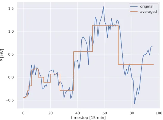
2.1 Comparison of U value distributions for Switzerland and for the member of EU28. The vertical line shows the identified U value for a monitored building located in Biel-Benken . . . 23 2.2 Example of logarithmically spaced aggregation, using 14 steps, of a de-trended

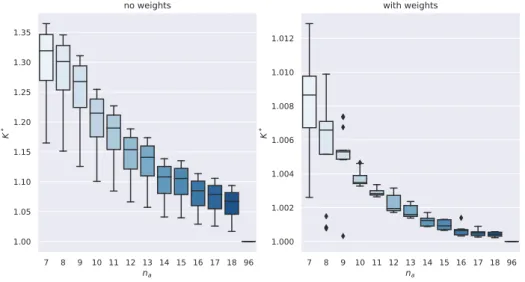
random walk. Blue: the original profile of 96 timesteps of 15 minutes each. Orange: logarithmic aggregations. . . 31 2.3 Performance gap shown in terms ofK∗, which is the ratio of the objective

func-tion value obtained by problem (2.41) and the non averaged formulafunc-tion (prob-lem 2.36), when using unitarywk (left) or equal tonk/T(right). The scores are plotted as a function of the battery capacity and E-rate, for an increasing number of aggregation stepsna. For both the cases the increase of capacity is more relevant reducing the performance gap, with respect an increase in the E-rate. . 33 2.4 Comparison of controller performances, when using unitarywk or equal to

nk/T. Each boxplot contains 16 observations, which are the fold-averages of the KPI, with respect to the capacity and c combinations. The scores are plotted with increasing number of aggregation stepsna. The scoreK∗is normalized with the KPI obtained by the non averaged formulation (problem 2.36). . . 34 2.5 Boxplots of the computational time of the nonuniform stepsize formulation, for

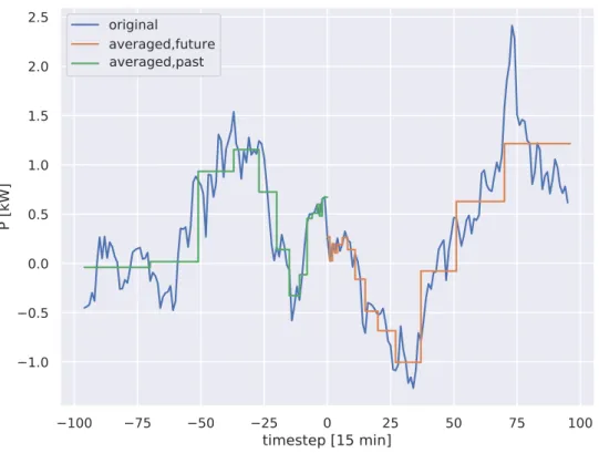
increasing number of aggregation stepsna. The computational time is normal-ized with the CPU time for the formulation withna=7. The median computa-tional time forna=7 was 0.028 seconds. . . 35 2.6 Example of logarithmically spaced aggregation, for the bins reported in 2.2, for

the regressor (green) and the target (orange). . . 38 2.7 Fitted parameters for the HW model, as a function of the step ahead . . . 42

(14)

2.8 Example of returned conditional pdfs, for the QRF, the HW and the bagging of ELM forecasters. First row: predictions for the 1st step ahead, that is, the mean value of the next 15 minutes. Second row: predictions of the last step ahead, that is, mean values of 7.75 hours, going from 16.25 hours ahead up to 24 hours ahead.Confidence intervals are relative to 10 linearly spaced quantiles between [0.05, 0.95] . . . 45 2.9 Evaluation of different regressors for multiple step ahead forecasting, in terms of

quantile skill score, RMSE,MAE and nMAE. Each boxplot contains 100 points, which are the results for each agent, mediated across the CV folds. Blue: QRF, direct. Red: RQRF, recursive. Yellow: bagging of ELM. Violet: detrended HW . . 46 2.10 KPIK_{r e}∗ (left), andK_er∗ (right), for different forecasters, as a function of

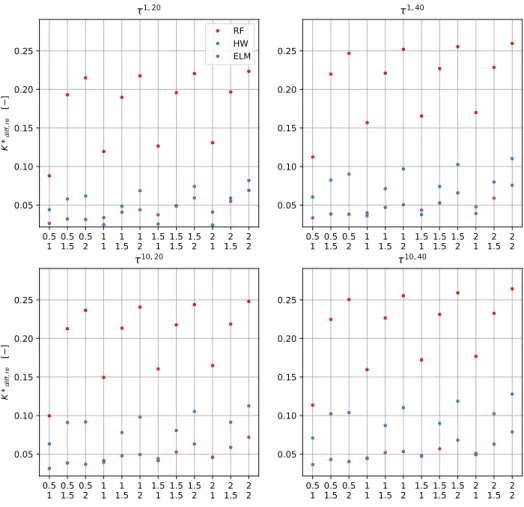
combi-nations of normalized battery capacity and E-rate. On the x axis, the first row refers to the E-rate, while the second one to the battery capacity normalized withE_nom∗ . Dots refer to the solutions of the deterministic solver, while crosses to the solution of the TBSMPC controller. . . 51 2.11 KPIK_{d i f f}∗ _,_{r e}, for different forecasters, as a function of combinations of

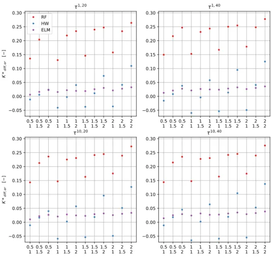
normal-ized battery capacity and E-rate, and different numbers of scenarios. On the x axis, the first row refers to the E-rate, while the second one to the battery capacity normalized withE_nom∗ . . . 52 2.12 KPIK_{d i f f}∗ _,_er, for different forecasters, as a function of combinations of

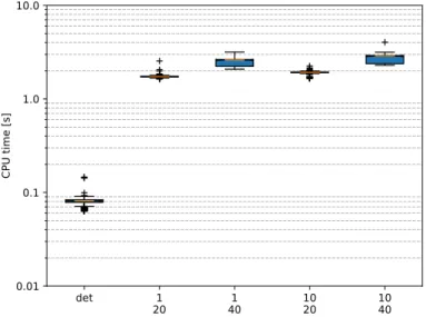
normal-ized battery capacity and E-rate, and different numbers of scenarios. On the x axis, the first row refers to the E-rate, while the second one to the battery capacity normalized withE_nom∗ . . . 53 2.13 Boxplot distributions of CPU times for the deterministic and stochastic

formula-tion using different tree structures (first row:µ1, last rowµ10). . . 54

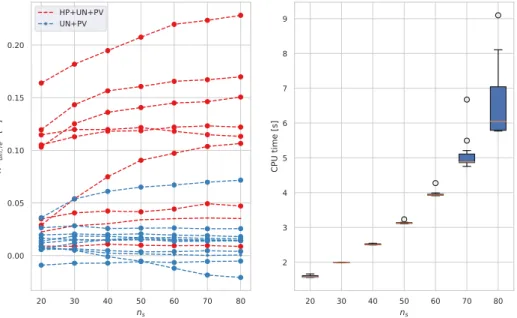
2.14 Example of power profiles from the two sets, during winter. On the left, a power profile from the first set, composed by a PV, an HP and uncontrollable loads. On the right, a profile from the second set, composed only by a PV and uncontrol-lable loads. . . 54 2.15 Left:K_{d i f f}∗ _,_{r e}for increasing number of scenarios. Each line represents a different

power profile. The red ones include an HP, while the blue ones are only com-posed by a PV plant and uncontrolled loads. Right: computational time boxplots for increasing number of scenarios, for the solution of a single optimization horizon. . . 55 3.1 AC power produced by 21 differently oriented virtual PV panels, during the first of

January, for the location of Biel-Benken, CH. The virtual PV panels’ orientations are obtained by generating a triangular mesh of an icosahedron on a unit sphere. 60 3.2 Example of 10 folds cross validation on the 80 days dataset. The dataset is divided

in 10 folds, each of 8 days. For each fold, the training set (green) is composed by 3 consecutive days each 4 days, while the test set (red) is composed by the remaining days. . . 64

(15)

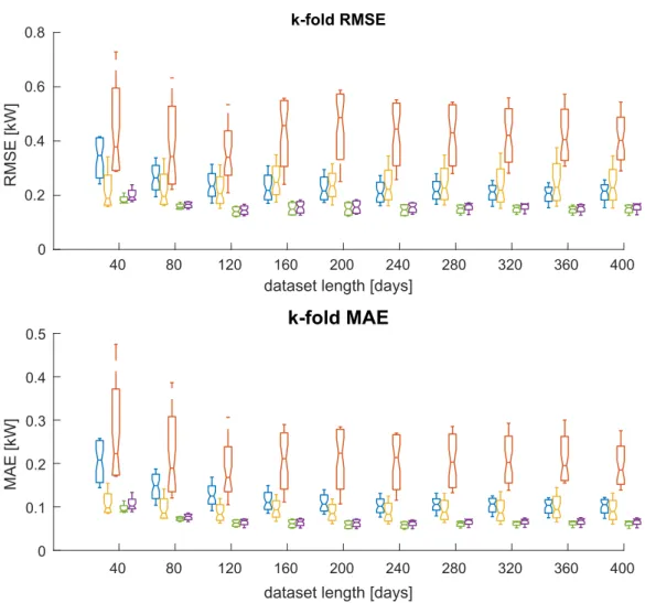
3.3 Boxplots of the RMSE and MAE based on the number of days of the dataset and on the method of prediction. Blue: 1Pˆp v, yellow:

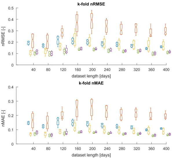
2_ˆ Pp v, red: 3_ˆ Pp v, green: 4_ˆ Pp v, violet:5Pˆpv. . . 65 3.4 Boxplots of the nRMSE and nMAE based on the number of days of the dataset

and on the method of prediction. Blue:1Pˆp v, yellow:

2_ˆ Pp v, red: 3_ˆ Pp v, green: 4_ˆ Pp v, violet:5Pˆpv. . . 66 3.5 Values of the identifiedωcoefficients for all the households, for the robust fit

regression (left) and for the blind identification (right), based on he number of training days, mediated over the cross validation folds. . . 67 3.6 nRMSE as a function of step ahead for perfect forecasts. Blue: base case. Red:

with PV model. Yellow: with PV model estimated withoutG H I. . . 70 3.7 nMAE as a function of step ahead for perfect forecasts. Blue: base case. Red:

with PV model. Yellow: with PV model estimated withoutG H I. . . 71 3.8 nRMSE for perfect forecasts (blue), perfect forecasts downsampled (green) and

real forecasts (bordeaux), for the base case (no PV models) . . . 73 3.9 RMSE of the forecast obtained using the PV models, normalized to the RMSE of

the base case. Blue: with PV model. Red: with PV model estimated withoutG H I. When using NWP forecasts, PV modeling results beneficial for the step ahead in which the NWP accuracy is higher (top), while consistently increasing for the case in which perfect forecasts are used (bottom). . . 74 3.10 RMSE of NWP forecastedG H I, as a function of the step ahead, normalized with

the total observed energy per step. . . 75 3.11 nRMSE as a function of step ahead for 1 hour downsampled perfect forecasts.

Blue: base case. Red: with PV model. Yellow: with PV model estimated without

G H I. The effect of modeling PV is negligible for the first 3 steps ahead. . . 76 3.12 ECDF of the horizon nRMSE for the base forecast and the two PV model forecasts,

for each household. The dotted lines are referred to the clear sky day dataset. . 77 3.13 ECDF of the horizon nRMSE for the base forecast and the two PV model forecasts,

for each household. The dotted lines are referred to the clear sky day dataset. . 78 4.1 RMSE for the base forecasters, the reconciled profiles withW equal to the

iden-tity matrix, and the reconciliation using the minT strategy. The first column refers to the mean RMSE across the whole hierarchy, the second to the error of the top level, and the third to the error in the bottom forecasters. . . 85 4.2 PV error selection mask for one day of observations, with 96 timesteps of 15

minutes each. The mask entries are 1 if in all the time window of that step ahead θaz>0. . . 86 4.3 Probability density of the absolute value of the correlation coefficient, as a

function of step ahead, for 100 simulated PV profiles. Left: with corrupted forecasts. Right: with perfect forecasts. . . 87

(16)

4.4 Distribution of the absolute value of the correlation coefficient, by means of quantiles (form 0.05 to 0.95), as a function of the step ahead. Left: 100 simulated heat pump profiles. Center: 100 simulated uncontrolled profiles. Right: 2200 measured mixed power profiles from the UK dataset. . . 88 4.5 Empirical a-priori pdf of the forecast error of the sum of 100 uncontrolled power

profiles, by means of quantile intervals. Upper left: assuming uncorrelated Gaussian errors. Upper right: assuming correlated Gaussian errors. Lower left: convolution of single pdf. Lower right: empirical distribution. . . 91 4.6 Empirical a-priori pdf of the forecast error of the sum of 100 PV power profiles, by

means of quantile intervals. Upper left: assuming uncorrelated Gaussian errors. Upper right: assuming correlated Gaussian errors. Lower left: convolution of single pdf. Lower right: empirical distribution. . . 92 4.7 Visualization of the steps of the proposed methods. On the left, the generation

of meteorological scenarios by means offm is depicted (top:G H I,bottom:T); the central part represents the deterministic output of the power forecasters, based on the set of received scenarios; the right part depicts the deterministic summation of thefiresponses, producing aggregate consistent scenarios, which are then used to retrieve the final pdf. . . 95 4.8 Reliability plots for the tree different methods of forecasting. First column:Ms,

second column:Mp, third column:Mc . . . 96 4.9 In-folds distributions of the quantile skill scores, RMSE and MAE, for modelMp

(blue) andMc(red), normalized with the same values fromMq . . . 97 5.1 Feasible sets for the space of two prosumers’ actions, for the constraint|x1+x2| <

Pin the case of individual policies (dark gray) and in the case of communication (light gray). Communication enlarges the feasible set, thus potentially improving the solution. . . 105 5.2 Example of topology identification using the IEEE European Low Voltage Test

Feeder. Small light gray dots represents the actual nodes in the grid. Big dark gray dots represents PQ nodes where measurements are available. Dashed lines are the actual physical connections, while dark blue lines are the identified connections. . . 107 5.3 Estimated pdfs of the computational time divided by the total number of agents,

as a function of the number of levels in the hierarchy. The vertical bar is the interquartile range, the horizontal line is the median. . . 109 5.4 Time series example, N = 10. Blue: forecasted profiles. Red: constraints. Grays:

solutions of the centralized and decentralized approaches. Top: state of charge for each battery. Middle: power profiles. Bottom: voltage profiles. . . 112

(17)

List of Tables

2.1 Characterization of the used forecasting methods. . . 42 2.2 Number of minutes for each step ahead. . . 43 2.3 Regressors for which the averaged history is passed to the forecasters (first

row), the ones for which the averaged future values is given (second row, NWP variables), and the ones for which only the value at the current time is given (third row) . . . 43 2.4 Number of houses per type of appliances. . . 43 2.5 Agent median computational training time for 2 months of data, for each

fore-caster. . . 47 3.1 Number of minutes for each step ahead. . . 68 4.1 Set of regressors for each type of forecaster . . . 94 5.1 Distributed control methods for OPF and DSM based on uncertainty formulation

and equilibrium formulation. . . 101 5.2 Distributed control methods for OPF and DSM based on decomposition method.101

(18)

(19)

Nomenclature

Acronyms

AD M M alternating direction method of multipliers

AOI angle of incidence

B RP balance responsible party

C+I consensus plus innovation

CC chance constraint

D−OP F distributed OPF

DE R distributed energy resources

DG distributed generation

D H I diffuse horizontal irradiance

D N I direct normal irradiance

DR Douglas-Rachford

DR demand response

DSM demand side management

DSO distributed system operator

DW Dantzig-Wolfe

E LM extreme learning machine

F B F Forward Backward Forward

F F T fast Fourier transform

G H I global horizontal irradiance

G N E generalized Nash Equilibrium

H P heat pump

HW Holt-Winters

I AM incidence angle modifier

i i d independent and identically distributed

I SO independent system operator

K P I key performance indicator

LV low voltage

(20)

M I MO multiple input multiple output

M I SO multiple input single output

M PC model predictive control

MV medium voltage

N E Nash equilibrium

nM AE normalized mean absolute error

nR M SE normalized root mean squared error

NW P numerical weather prediction

ODE ordinary differential equation

OP F optimal power flow

P F power flow

pF B preconditined Forward Backward

PV photovoltaic

QRF quantile regression forest

R M SE root mean squared error

RQRF recursive quantile regression forest

SB scenario based

SCC self consumption community

SM PC stochastic MPC

SOP F stochastic OPF

T B SM PC tree based stochastic MPC

T SO transmission system operator

UC unit commitment

U N uncontrolled loads

V CG Vickrey-Clarke-Groves

V N E variational Nash Equilibrium

W M welfare maximization

Chapter 1 - Background and state of the art

〈x,y〉 scalar product between x and y

² disturbance

ˆ

F empirical cumulative density function

prox(·) proximal operator

F σ−field M model N normal distribution X constraint set E expectation operator I indicator function

(21)

P probability measure

µ mean

Ω sample space

Φ Gaussian cumulative function

π node probability Σ covariance matrix σ standard deviation τ rooted tree Dt e testing dataset Dt r training dataset

F cumulative density function

f :Rn⇒Rn operator/map/multi-valued function

F−1 inverse cumulative density function (quantile)

l loss function

nb number of bootstrapped dataset

nobs number of observations

ns number of scenarios

p probability density function

q_α quantile of levelα

T prediction horizon

t time

t_endh ending time of hourh th_{st ar t} starting time of hourh

U uniform distribution

ui cost function of agenti

x decision variable

x∗ optimal solution

x₋i concatenation of all agents’ actions but the ones from agenti: [xT₁,xT₂, . . . ,x_iT₋₁,xT_i₊₁, . . . ,x_NT]T

Chapter 2 - Multi-step-ahead forecasting for demand response applications

α tilt angle of PV field

L _{direct sum operator}

† pseudoinverse opeartor

˙

m inlet mass flow

˙

Qbuo heat power due to buoyancy effect ˙

Qcond heat power due to conduction ˙

Qh heat power due to heating element (electric resistance) ˙

Ql oss heat power exchanged with the ambient

ηt combined module and inverter efficiency ˆ

(22)

λ Ridge regularization coefficient for the ELM

Dk,j set of descendants of node jat timestepk

U control variable constraint set

ED expectation with respect to the datasetD

θa,t azimuth angle of the sun at timet

θz,t zenith angle of the sun at timet

⊗ Kronecker product

Φx enthalpy flow inside the heating pipe, at positionx

σ(·) activation function for the ELM τµi,µj _{tree structure with}µ

inodes in the first step ahead andµjnodes in the last step ahead

θ matrix of output weights for the ELM

Ad discrete dynamics state matrix for the controlled system

Bd discrete dynamics control matrix for the controlled system

C heat capacity of the water layer

c(·) energy cost function

cp specific heat capacity of water

I radiation on a given surface

Ib direct radiation on a given surface

Id diffuse radiation on a given surface

Ig ground reflected radiation on a given surface

Ii,t oedinary differential equation

IST C reference irradiance under standard conditions

k thermal conductivity of water

K_{r e}∗ expectation of the ratio between the closed loop performance gap and the pre-scient controller’s performance

Kr e∗ expected ratio of the performance gap of the stochastic controller and the perfor-mance gap of the deterministic controller, w.r.t. the prescient controller

K∗

r e ratio between the expectation of the closed loop performance gap and the expec-tation of the prescient controller’s performance

K_{r e}∗ ratio between the expected performance gap of the stochastic controller and the expected performance gap of the deterministic controller, w.r.t. the prescient controller

K_i∗_,_j_,_n

a controller closed loop performance for a given E-rate, capacity and number

of aggregation steps, normalized with the performance of the uniform MPC formulation

Mx block diagonal matrix for the reduction of the regressors dataset

My block diagonal matrix for the reduction of the target dataset

na number of aggregated steps for the nonuniform stepsize MPC formulation

nk number of original steps which are used for thekt haggregation

nx number of regressors

(23)

pb energy buying price

ps energy selling price

S summation matrix for the battery operations

S(·) quantile skill score

Ta ambient temperature

Tcel l cell temperature of a given PV module

uamb equivalent thermal loss coefficient between the tank and the ambient

W matrix of inner layer wights for the ELM

wk objective function re-weighting coefficient for thekt haggregation

xst ar t initial state of the controlled system

Chapter 3 - PV modeling for power forecasting

²cl ratio between the estimated GHI and extraterrestrial irradiance in the reference period

ˆ

ω identified PV model coefficients

ˆ

ωbl PV model coefficients, blindly identified from composite power flow

Et extra-terrestrial irradiance at time t

Pl power consumption of the loads

Pm composite power measurement

st clear sky indicator at time t

Chapter 4 - Hierarchical forecasts for distributed control algorithms ˆ

Pbu forecast of the aggregated profile, obtained with a bottom up approach

F Fourier transform

ρi,j,k absolute value of the correlation coefficient between forecast errors of profilei andjat thekt hstep ahead

θel sun elevation angle

fm(·) forecast function for NWP scenario generation

Chapter 5 - Distributed energy markets

α repartition coefficient

λ Lagrangian multiplier

(24)

(25)

Introduction

Motivations of the thesis

The incremental deployment of decentralized stochastic generators at the low and medium voltage levels of the distribution grid introduces a number of new challenges for the safe operation of the network, like for example voltage fluctuations and line congestions [1; 2; 3; 4]. Among the proposed solutions to this problem, an active control of distributed loads and storage, also known as demand side management (DSM), has been widely suggested [5; 6; 7; 8]. For an effective management of the network through the actuation of distributed flexible loads and storage systems, it is imperative to be able to coordinate their actions efficiently. Substantial, authoritative work addresses the theme of DSM and demand response (DR) from a theoretical standpoint [9; 10; 3; 11; 12], analyzing the best strategies for agent coordination towards an optimal aggregate behaviour on single grid levels. But, as flexibility will be offered at different levels and will provide a number of services, from voltage control for the distributed system operator (DSO) to control energy for the transmission system operators (TSOs), it is important to make sure that these services will not interfere with each other. It is clear that offering services to a TSO or a balance responsible party (BRP) can very realistically have an impact on power quality, both locally and at a distance. While TSOs objectives are focused on the flawless operation of the bulk grid, (e.g. reserve scheduling and congestion management in the transmission grid), DSOs and independent system operators (ISOs) are more concerned with power quality in terms of bounded nodal voltages, line congestion, islanding of local portions of the grid and local dispatch. The coordination needed for such services implies substantial load correlation and openly challenges the traditional assumption of “statistical smoothing”, under which DSOs have designed their grids; let alone the effects of the ever-increasing penetration of photovoltaic (PV) systems at the low voltage level. At the same time, the stochasticity and volatility of distributed energy resources (DERs) power generation is pushing electricity markets towards smaller clearance times, with respect to the day ahead planning used in the Day Ahead Market. Furthermore, as DSM and DR rely on prosumers owned assets with small starting time compared to centralized power plants, the solution paradigm is shifting from solving unit commitment (UC) problems to the one of solving multistage stochastic problems, using a rolling horizon fashion. This paradigm shift

(26)

in the modality of grid usage requires a certain degree of system overhaul. In particular, one needs to ensure that DSM does not create congestions or voltage violations at any point of the distribution grid. A comprehensive approach towards the actuation of flexibility, taking into account its effects at different grid levels, is proposed in this thesis. In this work, I chose to investigate distributed control techniques for the problem of coordinating the flexibilities in the grid. Compared to centralized techniques, distributed control offers the advantage of being more scalable and allowing to preserve partially the privacy of the agents. On the other hand, distributed control presents a number of challenges, among which the need to decompose the optimization problem and distribute it among the agents, who need to solve parts of it locally, often on a hardware, which has limited computational power. To successfully apply distributed control techniques for the coordination of a set of agents represented by electrical loads or batteries, one needs to rely on the forecasts of each agents’ electrical consumption/production with relatively high time resolutions. Since both power consumption and DERs power production profiles have a daily seasonality, a 24 hours ahead planning is typically used. The high number of time steps, the frequency at which the problem must be solved, the number of agents to be coordinated (in the range of hundreds) and the limited computational power of the devices on which the distributed control problem is solved (smart meters), require a careful selection of both optimization strategy and forecasting algorithm. The efficient forecast of a high number of relatively small loads and generators is particularly challenging. Part of this thesis is specifically dedicated to the design and evaluation of forecasting techniques for production and consumption. Both the accuracy and the computational requirements of the proposed techniques is evaluated. A particular focus went on PV forecasting, since PV represents most of DERs. Another challenge when forecasting relatively small loads and generators is the lack of monitoring equipment. Often, PV production is not measured separately and it simply adds negatively to the aggregated power consumption. In this work, disaggregation techniques that allow disaggregating PV production from power consumption are proposed and evaluated. When multi objective optimization techniques are applied to optimize for both a local (e.g. single household level) and a global (aggregate power of a neighborhood) objective function, consistency in the forecasted power profiles is required. This means that the forecasts of the single agents should sum up to the forecast of their aggregate. This consistency is particularly challenging to obtain when considering probabilistic forecasts. For this reason I propose a method to retrieve probabilistic forecasts which are aggregate-consistent by construction, without the need of empirically modeling a large number of probabilistic interdependencies between forecasters, as the state of the art suggests.

Contributions and structure of the thesis

In what follows, the main contributions of the thesis are presented, referencing the chapters in which they are treated, grouped by the four problematics introduced in the motivation.

(27)

forecasting techniques with low computational requirements are compared to more sophis-ticated and computational intensive methods. In particular, we investigated the loss of performance of a deterministic model predictive controller (MPC) using forecasters of a computationally cheap parametric forecaster, with respect to a tree based stochastic model predictive controller (TBSMPC) exploiting conditional probability density functions provided by a quantile random forest (QRF).

• In section 2.2, a nonuniform stepsize MPC formulation is presented. Logarithmically spaced steps are used, and their number is systematically increased while evaluating the controller performance using synthetically generated residential power profiles. The aim of the control step reduction is twofold, lowering the controller computational time and both the forecasters training dataset and training computational time . We show that, when re-weighting the objective function for the length of the averaging bins, the maximum relative increase in the objective function with respect of the full formulation using 96 steps, is well below 1%, using only 10 steps.

• In section 2.3, two new forecasters with low training computational time and memory requirement are presented: a detrended Holt-Winter (HW) forecaster and a bagging of extreme learning machines. The HW provided strictly better a-priori performance for the first step-ahead forecasts, with respect to all the other models. When evaluating the forecasters a-posteriori, by means of closed loop performances of an MPC controller, the Holt-Winter forecasters shows performances which are close to the one provided by the best forecaster, with the advantage of being computationally cheaper. When the a-posteriori evaluation is done using a TBSMPC controller, the tests shown that the forecaster based on a QRF regressor consistently provide better performance, at the price of a higher computational time for the model training and memory requirements.

Influence of PV modeling on forecasting As a growing number of roof-mounted PV system is being installed, in section 3.2 we investigate the effect of exploiting physics-based PV models in order to forecast their power production. Forecasting PV power is of great importance for the future electrical grid, as more accurate power predictions allows to better handle abrupt rump up in regional power flow, due to change in cloud configuration, and ultimately permit to increase the number of PV plants which can be hosted in the distribution grid. Estimating physical models of existing PV systems in an automatic and unsupervised way, has the additional benefit of turning PV panels into irradiance sensors. In section 3.1.2 we introduce a new method to reconstruct theG H Iusing only AC power from a PV power plant. Chapter 2, treating these subjects, is partially based on the annexed papers:

[A] F. Sossan, L. Nespoli, V. Medici, and M. Paolone, “Unsupervised Disaggregation of Pho-tovoltaic Production from Composite Power Flow Measurements of Heterogeneous Pro-sumers,” IEEE Trans. Ind. Informatics, 2018.

(28)

[B] L. Nespoli and V. Medici, “An unsupervised method for estimating the global horizontal irradiance from photovoltaic power measurements,” Solar Energy, 2017.

The main outcomes of the thesis on this topic, contained in chapter 3, are the following:

• A methodology to blindly identify a physical model of PV power plants, starting from composite power signals, are introduced in sec 3.1. The different methods are explained in detail in paper A.

• In section 3.1.2, a new unsupervised method for estimating the GHI from AC photo-voltaic power measurements is introduced. The detailed procedure is presented in paper B, and its improved accuracy with respect to satellite-based irradiance estimations is reported, for two case study.

• It is shown how, combining physical models and QRF, the accuracy of predicting PV output from meteorological conditions increases significantly. Moreover, blindly identify the PV model starting from composite power measurements does not significantly decrease the prediction accuracy.

• It is shown how modeling PV does help to increase the forecast accuracy, only for steps ahead between 30 minutes and 12 hours, period in which NWP are more reliable.

Hierarchical forecasting techniques When applying DSM, we are typically interested in minimizing an objective function which depends on the aggregated power profiles of a group of agents in the distribution grid, while respecting grid constraints. This requires to separately forecast agents’ power profiles. In this case hierarchical forecasting techniques can be used to improve the forecasts’ accuracy. When we are interested in probabilistic forecasts, the problem becomes harder, requiring in general a multidimensional integral. The main contribution in hierarchical forecasting of this thesis, contained in chapter 4, are the following:

• In section 4.1, a new distributed method to reconcile forecasters at different levels of a hierarchical structure is presented. This method can be used to make forecasts done by different entities aggregate-consistent, thus usable in distributed control. The main advantage in redistributing the reconciliation is that private information which could be used by the base forecasters, is not disclosed. Furthermore, informations at upper levels of the hierarchical structure is only available by means of aggregate power profiles. • In section 4.2, a new method to obtain aggregated consistent pdfs for hierarchical power

forecasts is presented. We show that nontrivial methods for summing the bottom level forecasts’ pdf are needed especially in the case of high penetration of PV. In this case forecasting errors becomes dependent, due to imperfect NWP.

(29)

providing multiple ancillary services at different voltage levels of the distribution grid, and trustless coordination of agents. For example, an independent group of prosumers can provide congestion management at the MV level and voltage control at LV level for a DSO, sell its aggregated flexibility to BRPs to help them meeting previously committed power profiles on the spot or intraday market, or sell provide secondary or tertiary control to the TSO. Another interesting case is the one of self consumption community (SCC), in which a group of prosumers connected to the main grid through a single point of coupling can pay its electricity bill as a single entity. This means that SCCs are pushed to increase their self consumption in order to low their total energy expenses. These thematics are briefly introduced in chapter 5. We propose a multilevel hierarchical distributed algorithm, which makes use of voltage sensitivity coefficients in order to respect grid constraints. Since distributed control algorithm based on problem decomposition are prone to malicious attacks and manipulations [13; 14; 15], in this chapter we analyze the proposed algorithm and show it can be easily turned into a non-cooperative game with a unique Nash equilibrium. Moreover, we propose a method to enforce individual rationality, which is, the condition for which the energy market participants are always better off opting in.

The two subjects are separately treated in these two annexed papers:

[C] L. Nespoli and V. Medici, “Constrained hierarchical networked optimization for energy markets,” IEEE PES Innovative Smart Grid Technologies Conference Europe (ISGT-Europe), 2018.

[D] L. Nespoli, M. Salani, and V. Medici, “A rational decentralized generalized Nash equi-librium seeking for energy markets,” in 2018 International Conference on Smart Energy Systems and Technologies, SEST 2018 - Proceedings, 2018.

List of related publications The following publications are related to, but not included in this thesis.

• V. Medici, M. Salani, L. Nespoli, A. Giusti, N. Vermes, M. Derboni, E. Rizzoli, D. Rivola, “Evaluation of the Potential of Electric Storage Using Decentralized Demand Side

Man-agement Algorithms,” in Energy Procedia, 2017.

• L. Nespoli, A. Giusti, N. Vermes, M. Derboni, E. Rizzoli, and L. M. Gambardella, “Dis-tributed demand side management using electric boilers,” Computer Science - Research and Development, 2016.

• L. Nespoli, V. Medici, and R. Rudel, “Grey-Box System Identification of Building Thermal Dynamics Using only Smart Meter and Air Temperature Data,” 14th IBPSA Conf., 2015.

(30)

(31)

1

Background and state of the art

Part of this thesis concerns the evaluation of different forecasting techniques by means of optimal (stochastic) control performance. This evaluation requires the knowledge of a broad variety of topics, which however, share the common mathematical background of optimiza-tion. For instance, in chapter 2 we will use a quadratic cost function for the evaluation of different probabilistic forecasters, which is justified by the common need of evaluating proximal operators for different class of distributed control algorithms. Lagrangian duality framework is used in chapter 4 to distribute the technique of hierarchical forecasting reconcil-iation, as well as to obtain the distributed control algorithms in chapter 5. Monotone operator theory, on which the alternating direction method of multipliers (ADMM) is based, is used to demonstrate the uniqueness of Nash equilibrium for the class of non-cooperative games generated by sharing problems in chapter 5. The concept of rooted trees is used in chapter 5 in order to formulate a multilevel hierarchical coordination algorithm spanning multiple voltage level of the distribution grid, as well as in the tree based stochastic MPC framework to have a compact description of the evolution of the control problem’s uncertainties. For this reason, this chapter gives an overview on the interconnections between forecasting, stochastic and distributed control, and aims at grouping the common mathematical tools which have been used in different parts of the thesis.

1.1 General patterns - optimal power flow

One of the key problems faced by independent system operators (ISOs) when considering intra day operation or day-ahead market clearing is the unit commitment problem (UC) [16], in which the operations of a set of generators has to be planned in advance, and the ISO commits to the optimal scheduling for the next day. Usually, the UC incorporates some kind of optimal power flow problem (OPF) [17; 18; 19; 20]. Based on the specific constraint which are considered, the OPF problem is known by different names, as network constrained, security constrained, alternate current, direct current OPF. A review on the different kinds of OPF formulations can be found in [21]. As the power generation get more decentralized and uncertain, due to DERs and REs, ISOs and and distribution system operators (DSOs) have

(32)

moved from the traditional deterministic OPF and UC formulation, to ones which incorporate higher levels of uncertainty and to decentralized solution strategies. A comprehensive review on the different state of the art methods to deal with uncertainty power system studies and stochastic OPF (SOPF) can be found in [22; 23], while [24] present a more specific review on stochastic formulations of UC problems. In [25] a partial survey on distributed approaches to UC, OPF, optimization and approximated PF formulations is presented.

Several formulations of the OPF exist, based on the type of the considered grid (high or medium voltage, radial or meshed, balanced or unbalaced) and control objective. In order to motivate the modeling choice that I use in chapter 5, in the following I introduce the general formulation of the OPF. Given an electrical grid composed by a set ofnbuses (or nodes), we refer to the optimal power flow problem to the task of minimizing an objectivef(Sc), which is function of the complex powersSc∈Cnc injected in the set of controllable buses

N

c=1, 2..,nc,nc<n, subject to bus voltage consistency, power balance and operational constraints.

min Sc⊂S f(Sc) s.t. I=Y V S=V¯I∗ V ∈

V

, S∈

S

, I∈

I

(1.1)

where¯is the Hadamard product,Y is the admittance matrix,I∗ stands for the complex conjugate of the currents’ vector and

V

,

S

and

I

are operational constraint sets for the voltages, complex power and currents. While the OPF described in (1.1) uses the so called bus injection model, an equivalent formulation known as branch flow model can be found in the literature [26]. The latter is especially useful for the formulation of convex relaxations of the OPF [27], or for its distributed computation [28]. Unfortunately, while (1.1) can be reliably solved for high and medium voltage grids, where the lines’ parameters needed to obtain the admittance matrixY are usually known, this is not the case for low voltage networks. Furthermore, solving (1.1) requires the knowledge of current and voltage phasors for the controlled nodes in the grid. In this thesis I assume that phasors’ measurements are not available, and that the OPF can only be solved relying on magnitude measurements ofV andI, provided by residential smart meters. For these reasons, instead of solving the OPF directly, chapter 5 considers a relaxed formulation of (1.1), in which the knowledge of phasors’ angles is not needed. The relaxed formulation is based on the voltage sensitivity coefficients, which are the first order approximation of the power flow equations. These are introduced in details in subsection 5.2.1, where limitations of this formulation are also discussed. Under these assumptions, the

(33)

relaxed OPF becomes: min P,Q f(Pc) s.t. |V| =V0+Kp∆P+Kq∆Q |V| ∈

V

, P∈

P

, Q∈

Q

(1.2)

whereKpandKqare voltage sensitivity coefficients matrices associated with active (P) and reactive (Q) power,V0is a reference voltage magnitude vector and∆is the first order discrete

time difference operator.

1.2 Mathematical preliminaries and notation

Through the thesis we will make use mathematical concepts for which different notations are reported in the literature. For example, the nomenclature for probability spaces and vector maps are often inconsistent through the literature. Here the mathematical notation used in the rest of the thesis, which was made as consistent as possible, is reported.

Random variablesxdefined on a probability space (Ω,F,P) whereΩis the sample space

F is aσ−field, andPis a probability measure, are reported without subscripts, whereas the same variable with a subscript,xk, denotes a realization, which is, a random draw from the probability density function (pdf )p(x). The cumulative density function (cdf ) of a continuous pdf is

F(z)=P(x<z)=

Z z

0

p(x)dx (1.3)

while the empirical cdf is defined as

ˆ F(z)= 1 1+nobs nobs X k=1 I{xk<z} (1.4)

whereI{·}is the indicator function andnobs is the number of observed realizations ofx. Theα quantile ofFxis defined as the generalized inverse ofF

q_α=F−1(α)=i n f{z∈R,F(z)≥α} (1.5)

Given a multivariate random variable,F(x|y) andp(x|y) are the conditional cdf and pdf, respectively, for which the Bayes’ theorem holds:

(34)

wherep(x,y) is the joint pdf andp(x) is also known as the marginal pdf ofx. The expectation operator is denoted asE[·], andED[·] denotes the expectation with respect to the dataset

D. The set of integers {k1,k2, ...kN} is denoted asN[k1:kN], and [xk] N k=1=

£

x₁T,xT₂...x_kT¤T is the collection ofxkfromk=1 toN. f :Rn→Rindicates a real value function, whilef :Rn⇒

Rn indicates an operator, also known as a map, multi-valued function or correspondence, mappingRn onto itself. For example£

∂kV(x,yk) ¤N

k=1 indicates the subdifferential of the

mapV(x,y) :Rn⇒Rn. The scalar product is denoted as〈x,y〉, or equivalentlyxTyfor the Euclidean space. The notationkxk22stands for the sum of squares ofx, whilekkpindicates the pnorm.

1.3 Stochastic model predictive control formulations for power

sys-tems

As anticipated in the introduction, since DSM and DR rely on prosumers’ owned assets with small start up and shot down times and costs compared to highly inertial traditional power plants, in order to reliably control these assets in the LV or MV gird, there is no need of committing to a certain scheduling of the latter [29]. For this reason in this thesis we will focus on the optimization of intra-day operations, and we won’t solve the UC problem, which is usually formulated as a two stage stochastic program and solved via L-shaped or Bender decomposition method, but we will restrict the study to stochastic OPF formulations. Considering multiple timesteps, both the previously introduced versions of the OPF, (1.1) ad (1.2), can be expressed as:

x∗_k=argmin x∈X E "_T X t=1 l(xt+k|k,²t+k|k) # (1.7)

whereEis the expectation operator over the random variable², which is defined over the prob-ability space (Ω,F,P),xis the decision vector (containing both states and control actions),

X is a bounded set, representing (probabilistic) operational constraints,T is the number of timesteps in the control horizon andlis a loss function to be minimized. We stress out that, since the objective function (and possiblyX) depends on², the optimal decision variable

x∗

k will also depend on the disturbance². For intra-day optimization, (1.7) is intended to be applied in a receding horizon fashion, thus that we can draw from the vast literature on stochastic MPC (SMPC). In general, due to lack of knowledge and unboundedness of the sam-ple spaceΩ, problem (1.7) is intractable, and must be therefore approximated. Three main strategies to approximate the stochastic control problem (1.7) are present in the literature and we briefly review them in the following. Namely, they are chance constraint (CC) analytic approximation, scenario based (SB) SMPC and tree-based (TB) SMPC. It must be noted that system operators are usually interested in solving a robust optimization problem rather than a stochastic one. Indeed the distinction between robust and stochastic optimization rely on how

(35)

we define the disturbance²and the constraint setX (as a function of²). Robust optimization usually considers an unknown distribution of², but a bounded sample spaceΩ, such that ²∈[²mi n,²max]. A solution is than found for whichx∈X(²) is satisfied for all the values of

²∈Ω. In other words, robust optimization find the optimal solutionx∗ considering worst case scenarios in terms of the disturbance, which is a wise optimization strategy in the case in which a violation of the constraint set implies irreversible damage to the operated system, as is usually the case in power grids. The CC approach tries to enlarge the feasible set of the solution, allowing probabilistic violations of the constraint set, making some assumptions on the pdf of². These assumptions are avoided in the SB approach, which uses a number of scenarios to model². Basic SB optimization do not uses chance constraints, that is, all the scenarios add hard constraints to the main problem. Anyway, is easy to see that a link exists between the number of considered scenarios and the probability to respect the constraints in the worst case. Indeed, as the number of scenarios increases, the solution under SB optimiza-tion approaches the one obtained using robust optimizaoptimiza-tion. For the three aforemenoptimiza-tioned strategy, only one vectorx∗_{is retrieved, which contains the optimal actions to apply to the}

controlled system up to timek+T. A third way of taking into account uncertainty is to encode ²into a disturbance tree, spreading with increasing time. This technique, TBSMPC, allows to represent the natural evolution of uncertainty, which typically increases as we consider further points in time, and to retrieve a rooted tree of control actions, of which only the first component is actually applied. In the following we briefly introduce them in order to motivate the use of TBSMPC in the rest of the thesis.

Analytical approximations of chance constraints Instead of strictly requiringx∈X for all possible realizations of², we can relax this hard constraint and reformulate it in terms of probabilistic constraints, also known as chance constraints:

x∗_k=argmin x E "_T X t=1 l(xt+k|k,²t+k|k) # s.t. : P[x∈X]>1−δ (1.8)

Unfortunately, also problem (1.8) is in general computationally intractable [30], especially whenX contains more than one constraint (e.g., it’s a polytopic), joint probabilistic con-straints would require the computation of a multidimensional integral over an unbounded probability space, and must be therefore approximated, for example, using convex analytic approximations, as in [31]. A more straightforward result is available in the case of a polytopic CC:

P£

gTx≤h¤

≥1−δ (1.9)

If the expected value and covariance matrixW of the disturbance are known, the Chebyshev -Cantelli inequality can be used [32; 33], which guarantees that (1.9) is (conservatively) satisfied

(36)

if

gTx≤h−

q

gT_{W g f}₍_δ₎ _(1.10)

where f(δ)=p(1−δ)/δ. Condition (1.10) can be made less conservative under Gaussian assumption of², usingf(δ)=N−1(1−δ). Given the results in [34], under the assumption of lognormal distribution, in [35] joint polytopic CC are conservatively reformulated as a set of single deterministic constraints. Another notably approximation, given the results in [30], in the case of disturbance generated by i.i.d. Gaussian random variables and SMPC with affine disturbance feedback is presented in [36].

Scenario based stochastic optimization When no assumption on the disturbance²can be made, or the CC formulations result in a too conservative control problem, one can revert to sampling based methods [31]. In scenario based SMPC, a number of scenarios is drawn from a stochastic process, or obtained by sampling with the methods explained in section 1.4. In scenario based SMPC, the probabilistic constraint in 1.8 is replaced with a set of deterministic ones: x∗_k=argmin x E "_T X t=1 l(xt+k|k,²it+k|k) # s.t. : x+²it+k|k∈X ∀i∈N[0,Ns],∀t∈N[0,T] (1.11)

where²i_t₊_k_|_kis theit hscenario of the disturbance at timet. It is easy to see that, as the number of scenarios increases, if the scenarios are drawn from the exact pdf of the disturbance,x∗

k will tend to the solution of a robust optimization problem. In order to loose the constraints, and obtain a less conservative solution, the number of scenarios must be carefully evaluated. It can be shown that the number of scenariosNswhich guarantees that the probabilistic constraints in (1.8) is satisfied with reliabilityδ, can be found analytically [37; 38]. The authors in [39] present a review on methods to encode chance constraints in SBMPC.

TBSMPC Instead of approximating problem (1.7) with a set of scenarios, we can describe the temporal evolution of the disturbance²with a rooted tree, denoted asτ. In this way we can retrieve a tree of control actions, with the same structure of the disturbance characterization. In other words, this method returnsnsoptimal control vectorsx∗, wherens is the number of leaves in the tree structure. Intuitively, this approach would result in a less conservative control with respect to the SB approach, since we can optimize over a greater number of control actions, each of which considers a branch in the evolution of the disturbance tree. This allows to take less conservative actions as the number of considered scenarios (or tree leaves) increases, as opposed to the SB approach. On the other hand, as in the SB approach, constraints in each branch of the tree are treated as (hard) deterministic constraints, meaning that increasing the number of leaves lead to consider extreme events as in robust optimization.

(37)

This method originates from the multistage stochastic programming [40; 41] literature, which is an extension of two-stage stochastic programming. When applied to MPC, this technique is also known as TBSMPC, and has been successfully applied in the literature to a broad class of problems, from intra-day energy management, to dynamic option hedging and drainage water systems control [42; 43; 44; 45; 46]. In [47; 35] two comparisons with numerical results of SBMPC and TBSMPC are presented. Different approaches can be adopted in order to retrieve the scenario tree used to describe the disturbance of the problem. This is usually obtained by clustering a high number of scenarios, which can be obtained with the method described in 1.4. The problem of generating an optimal tree from a set of scenarios, in the sense of minimizing the distance between distributions, is NP hard [48], and thus the scenario reduction could result in a high computational time when the number of original scenariosNs and the length of the considered horizonHare high. In the rest of the thesis we have adopted the backward reduction algorithm described in [49; 41], which uses a greedy strategy in order to minimize the Kantorovich distance between the trees and the original sets of scenarios. The probabilities of reaching each node from the root,πi, are found aggregating the probabilities of the originally merged scenarios, which by construction guarantees that:

µk X i=1

πk,j=1 (1.12)

wherek is the step ahead, andµk is the number of nodes for the stepk. In order to give a flexible description of the resulting rooted tree, the algorithm has been rewritten in python and coupled with the networkx package, which encodes the disturbance structure in a directed acyclic graph (DAG), allowing to use high level graph searches queries (e.g. list the ancestors of a given node). An example of scenario tree representation is shown in Fig. 1.1. The code is freely available at https://gitlab.com/supsi-dacd-isaac/scenred.

1.4 Multivariate probabilistic forecasting

Conditional pdfs can then be used to create scenarios, which are used in scenario based stochastic optimization, as explained in 1.3. Scenarios can be produced in different ways, depending on the type of algorithm used for obtaining the posterior pdf. In chapter 2 we will use three different techniques, which we introduce here. We don’t want to model the error with a particular probability distribution, since this will require to introduce assumptions in the analysis of the forecasters performance. We will only use non-parametric techniques for the production of the scenarios.

Bootstrap Bootstrap [50] was introduced to perform non-parametric inference on inde-pendent and identically distributed (iid) data, and lately become a very popular method for assessing statistical accuracy and model fitting [51]. The bootstrap consist in repeatedly drawing with replacement from a datasetD, in order to estimate some relevant statistical properties. Since in this thesis we are interested in power forecasts, which typically shows a

(38)

102 ₁₀3

time ahead [min] 4 3 2 1 0 1 2 3 4 Power [kW] Scenario DAG 2 1 0 1 2 Power [kW]

Figure 1.1 – Example of scenario reduction results and encoding of the scenario tree into a DAG. Left: 200 scenarios generated for the prediction of 24 hours ahead power profile of a building. Blue lines: original scenarios. Black lines: scenario tree. Right: the same scenario tree, depicted as a DAG. The size of the dots its proportional to the intra-step probabilities.

daily seasonality, we slightly modify the bootstrap technique to take this into account. In order to generate statistically consistent scenarios for the power prediction, we fit a forecaster model

M on a training datasetDt r, and then we retrieve the forecaster’s error onDt r,²t r∈Rnobs,t r×T, wherenobs,t r is the number of observations in the training set andT is the horizon of the prediction. The scenarios for each of thenobs,t eentries of the test datasetDt e, on which the control policy is then evaluated, are retrieved performing bootstrap on²t r, based on the hour of the day.