Stefanie Kalus, Philipp Sämann, Michael Czisch
& Ludwig Fahrmeir
fMRI activation detection with EEG priors
Technical Report Number 146, 2013 Department of Statistics
University of Munich
fMRI activation detection with EEG priors
S. Kalusa,∗, P.G. S¨amannb, M. Czischb, L. Fahrmeira
aDepartment of Statistics, Ludwig-Maximilians-University, Ludwigstr. 33, 80539 Munich, Germany
bMax Planck Institute of Psychiatry, Kraepelinstr. 2, 80804 Munich, Germany
Abstract
The purpose of brain mapping techniques is to advance the understand-ing of the relationship between structure and function in the human brain in so-called activation studies. In this work, an advanced statistical model for combining functional magnetic resonance imaging (fMRI) and electroen-cephalography (EEG) recordings is developed to fuse complementary in-formation about the location of neuronal activity. More precisely, a new Bayesian method is proposed for enhancing fMRI activation detection by the use of EEG-based spatial prior information in stimulus based experimen-tal paradigms. I.e., we model and analyse stimulus influence by a spatial Bayesian variable selection scheme, and extend existing high-dimensional regression methods by incorporating prior information on binary selection indicators via a latent probit regression with either a spatially-varying or constant EEG effect. Spatially-varying effects are regularized by intrinsic Markov random field priors. Inference is based on a full Bayesian Markov Chain Monte Carlo (MCMC) approach. Whether the proposed algorithm is able to increase the sensitivity of mere fMRI models is examined in both a real-world application and a simulation study. We observed, that carefully selected EEG–prior information additionally increases sensitivity in activa-tion regions that have been distorted by a low signal-to-noise ratio.
Keywords: EEG, fMRI, activation probabilities, Bayesian spatial modeling, Markov Chain Monte Carlo sampling, hierarchical model
∗Corresponding author. Phone: +49 89 2180 6254
1. Introduction
Recording electrophysiological data simultaneously with functional mag-netic resonance imaging (fMRI) targets at combining the advantages of both modalities to gain deeper insight into brain functioning. Recently, extensive experimental and methodological research has been done to achieve this goal (see Mulert and Lemieux, 2010, for a compelling review). Both measurement techniques capture neuronal activity. Scalp electroencephalography (EEG) measures the summed activity of postsynaptic currents. Hereby, time series of electrical activity are recorded from multiple electrodes placed on the scalp. fMRI is one of the most recently developed and at present most popular form of noninvasive imaging of human brain activity. Just recently, celebrating 20 years of fMRI, an entire special issue was released by the NeuroImage jour-nal (Bandettini, 2012) demonstrating the popularity of the fMRI technique. fMRI also captures neuronal activity but in a more indirect way than EEG: Electrically active neurons are subject to a higher energy demand leading to an increase in blood flow into active brain regions. fMRI is based on the blood oxygenation level dependent (BOLD) effect and mirrors the changes in cerebral perfusion of capillaries with oxygenated blood. The fMRI tech-nique provides a time series of three-dimensional images of the brain. Both modalities, EEG and fMRI, are based on brain processes related to neuronal activity. Therefore, activated brain regions can be located by analysing both fMRI and EEG data.
EEG and fMRI data differ substantially by their corresponding generative process and also capture different aspects of neuronal activity, but neither captures all. For being recorded at the scalp surface, electric events in deeper brain regions, which are detected by fMRI, emerge as damped oscillations in the EEG and are hard to localize. On the contrary, signals recorded by EEG need not necessarily be identifiable in the simultaneously recorded fMRI time series. For instance, no explicit BOLD response was identified for some short-lasting EEG signals with high amplitude, as e.g. K-complexes. See Ritter and Villringer (2006) and Daunizeau et al. (2010) for a more detailed discussion of situations where discrepancies between concurrent fMRI and EEG recordings emerge.
The main motivation for developing statistical methods for the fMRI-EEG data fusion lies in compensating shortcomings—related to technical issues as well as the biophysical generation process—of one technique by adding information from the other to gain a deeper insight into brain
func-tioning. A close coupling between measuring EEG and fMRI data seems indispensable for this. Therefore, in the last couple of years, recording EEG simultaneously with fMRI has become firmly established. For this to happen, several technical challenges had to be overcome (Ritter and Villringer, 2006). Statistical methods that aim at combining EEG and fMRI face the chal-lenge of integrating two data types that differ strongly in their structure as well as their generative process. Basically, so far, three different analy-sis approaches to multimodal integration have been proposed (Laufs et al., 2008; Daunizeau et al., 2010; Rosa et al., 2010). We distinguish between
(i) EEG-to-fMRI approaches, where the fMRI signal is correlated with an
EEG-defined event or feature to gain information on the location of
electro-physiological phenomenons, (ii) fMRI-to-EEG approaches, where the spatial
information of the fMRI is used for a (spatiotemporal) source reconstruction
of the EEG and (iii) symmetrical approaches, usually referring to the use of
a common forward or a generative model that explains both EEG and fMRI data.
In this work, this set of approaches is extended by introducing a new type of method: an EEG-informed fMRI activation detection method. It is based on a high-dimensional fMRI regression model, which is also the
basis for (i). In preparation for incorporating EEG information, a suitable
uninformed fMRI activation detection method was developed. It grounds on ideas of Smith et al. (2003) and Smith and Fahrmeir (2007), who suggested to use a Bayesian variable selection approach and model averaging techniques to assess brain activity. Activity is, thereby, assessed locally at each voxel. A voxel is said to be active—in a narrower sense, to be responsive—if its fMRI signal trajectory responds to stimuli. That is, a voxel is active when a predictor component describing stimulus presentation has a significant effect on the fMRI signal. Alternatively, in terms of Smith et al. (2003), a voxel is said to be active if the inclusion of the stimulus predictor component plays a role in explaining the fMRI signal. To assess voxelwise activity, Smith et al. (2003) introduced voxelwise binary activation parameters in the form of selection indicators for the stimulus component and inspected the size of corresponding selection probability estimates, which serve as activation probability estimates. To account for the correlation between neighbouring voxels, estimation of activation probabilities was regularized by an Ising prior. The authors even provided a way to incorporate external prior information. This prior information, however, had to be available in the form of prior probability maps.
In this work, we extend the work of Smith et al. (2003) by providing means to include general prior activation information in continuous or bi-nary form. For this, we replace the Ising prior with a latent, spatial probit regression stage that accomplishes the mapping between general variable val-ues and probability estimations. For uninformed fMRI activation detection, the probit regression predictor consists of a spatially-varying intercept only (similar to the work of Smith and Smith, 2006). For EEG-informed fMRI activation detection schemes, spatial EEG information can be included as a further variable—possibly with a spatially-varying effect. To adjust for corre-lations within spatially-varying effect vectors, an intrinsic Gaussian Markov random field (IGMRF) prior was used.
Bayesian posterior analysis is based on a Markov Chain Monte Carlo (MCMC)-approach that allows to directly calculate all parameters and fea-tures of interest. In particular, the marginal posterior probability for activa-tion at each voxel is of interest, because it can be thresholded to provide an activation map.
In comparison to previous methods, our approach has several significant advantages. It shares several advantages of the Ising model (see Smith et al., 2003): First, our Bayesian formulation allows the explicit modelling of the probability that a voxel is activated, which circumvents either the
prob-lematic interpretation of frequentist p-values in classical approaches or the
counterintuitive selection of an activation threshold on the level of Bayesian activation amplitude effect estimates (Friston et al., 2002). Second, it incor-porates spatial correlations at the level of activation probabilities, which are the parameters of interest, and not just indirectly on the level of activation effects as, for example, in G¨ossl et al. (2001), Penny et al. (2005) and Groves et al. (2009). Third, because the posterior distribution incorporates the spa-tial structure of an IGMRF prior, there is no need for spaspa-tial adjustments in a postprocessing step.
Above that, our approach possesses a major advantage over the Ising model. Our modelling formulation allows to incorporate very general forms of prior information, which can be used to enhance fMRI activation detection. The intended use of our approach is to incorporate EEG-prior activation information in the form of 3D source reconstruction maps (Michel et al., 2004), though any kind of external prior information can be used as long as it is available as a single 3D map with activation information. The scale of the contained measurements is quite arbitrary: Voxel values can be binary or continuous. We generally assume, however, that larger values indicate
activation. As a EEG-fMRI data fusion technique, our approach is related to
(i) for being based on fMRI regression, but does not simply search for brain
regions showing a correlation with EEG features. Our approach extends fMRI regression by adding spatial EEG information to activation detection. In Kalus (2012) and Kalus et al. (2013), we have seen that our uninformed fMRI activation scheme has superior performance compared to classical SPM and the Ising model. They have highly increased sensitivity without losing their high specificity level and possess excellent edge-preserving properties. Hence, they can be considered to be an appropriate reference for examining the usefulness of EEG-enhanced schemes, which we propose in this work.
We will show that our EEG-enhanced fMRI activation schemes are ap-proximately as sensitive as our uninformed algorithms. This hints at the usefulness of our enhanced approaches and is a prerequisite for their intended purpose. These procedures are developed to compensate a low signal-to-noise ratio in the fMRI signal, which is often a problem in event-related designs,
to (a) make EEG phenomenons visible otherwise not detected and (b) bring
out activation regions more clearly when activation regions are blurred by noise. Though 3D maps derived by EEG source reconstruction methods have a low spatial resolution, they provide complementary information on the lo-cation of neuronal activity. To make use of EEG information without being biased by inaccurate location information, EEG-enhanced detection schemes need to be robust against prior misspecifications. Our developed algorithms ensure this for adapting to the level of EEG and fMRI congruency within the brain. This is achieved at the expense of a sensitivity increase. However, we identified data settings in which a substantial performance gain could be achieved compensating activation loss due to noise.
For researchers that want to use either the uninformed or EEG-enhanced fMRI activation scheme, we have implemented a user-friendly, computation-ally efficient software library making all discussed Bayesian algorithms
avail-able. The software is freely available as R packageRfmrieeg. Alternatively,
C++ source code is provided for a binary CfmrieegMain program. Both
kinds of software packages can be obtained from the author.
The rest of the paper is organised as follows. In the Methods section (Sect. 2), we first describe the basic fMRI general linear model used conven-tionally for activation detection (Sect. 2.1) and then describe how this model can be extended to incorporate external EEG information within a Bayesian hierarchical model by specifying suitable priors (Sect. 2.2). Bayesian model inference is outlined in Sect. 2.3. After providing the methodological
back-ground, we present results obtained on an event-related fMRI data set from an acoustic two-tone oddball design (Sect. 3). Simulation results derived from a modified version of the application dataset are shown in Sect. 4. In the Discussion section, we outline the main qualities and findings of our model and suggest starting points for further work.
2. Methods
2.1. The fMRI regression stage
fMRI data consist of signal time series yi,t, t= 1, . . . , T, recorded at each
voxel i = 1, . . . , N of a three-dimensional brain image. Detection of brain
activity is usually based on voxelwise regression models of the form
yi,t= fbase(i, t) +fcon(i, t) +fstim(i, t) +i,t. (1)
In (1), fbase(i, t) is the baseline trend, fcon(i, t) is the effect of confounding
covariates, fstim(i, t) is the effect of the (transformed) stimulus, and i,t is
the random error term at voxeliand timet. In the following, we discuss the
components of the fMRI regression model (1) in detail.
The baseline term fbase(i, t) corrects for slow periodic variations and drift
either inherent to the scanning procedure or connected to non-paradigm
cor-related periodic variations. Thus,fbase(i, t) serves as a highpass filter. In this
work, it is chosen to consist of a discrete cosine transform (DCT) set (Friston et al., 2008, p. 123) as in SPM. In contrast to SPM, but conceptually equiva-lent, the highpass filter in our modelling approach enters the regression stage
directly as a linear combination of basis functions fbase(i, t) = x(1)(t)0β(1)i
with basis functions x(1)(t) = (x(1)
k (t), k = 1, . . . , p1)0 and weights β(1)i =
(βi,k(1), k= 1, . . . , p1)0.
The second term fcon(i, t) accounts for further confounding effects like
for example movement related artifacts or brain tissue-specific properties capturing effects from cardiac and respiratory cycles, which are not captured by the highpass filter. It is assumed, that according information is available
in form of several univariate, global variables with valuex(2)(t) = (x(2)
k (t), k=
1, . . . , p2)0, at timet. The corresponding voxelspecific effect vector (βi,k(2), k=
1, . . . , p2)0 is denoted as β(2)i , so thatfcon(i, t) =x(2)(t)0β(2)i .
The regression component fstim(i, t) includes the transformed stimulus
time series of a given type. The fMRI signal represents aggregated and time delayed neuronal activity, which in turn has a close correspondence
to the stimulus presentation. Therefore, the stimulus time series has to be transformed to the level of the fMRI response to obtain models that more closely resemble the observed fMRI signal thus yielding a better fit. In this work, the focus is on modelling event related stimuli, although only minor changes have to be made to incorporate block designs into the framework.
We follow an approach proposed by Josephs et al. (1997) using the concept of mathematical convolution:
fstim(i, t) =
Z τmax
0
hrf(i, τ)u(t−τ) dτ
where the function u(t) describes the given time course of neuronal activity
andhrf(i, τ) is the unknown hemodynamic response function (HRF) at voxel
i. To estimate hrf(i, τ), a flexible modelling strategy with basis functionsBk
and corresponding voxelspecific weightsβi,k(3) is applied:
hrf(i, τ) =
p3 X
k=1
βi,k(3)Bk(τ).
This approach leads to a flexible and data driven estimation of the voxelspe-cific functional form of the hemodynamic response. Different choices of basis sets exist (Henson et al., 2001). We focus on the canonical basis function set (Friston et al., 2008, pp. 181), which is the default choice in SPM. We use the functional form of the canonical HRF as written down in Kalus (2012), pp. 41.
The time series of neuronal activity u(t) is set equal to the signal time
series, which is modelled as follows: Suppose we have event related stimuli of
one type at timesτ1, τ2, . . . , τM. A stimulus at timeτmis modelled via a dirac
delta functionδ(t−τm), i.e. a stick-function, so that u(t) =
PM
m=1δ(t−τm).
With this modelling strategy, the stimulus predictor for all presented stimuli is linearized with respect to unknown HRF effects:
fstim(i, t) = p3 X k=1 βi,k(3) M X m=1 Bk(t−τm) | {z } =x(3)k (t) =x(3)(t)0β(3)i , wherex(3)(t) = (x(3) k (t), k= 1, . . . , p3)0 and β (3) i = (β (3) i,k, k= 1, . . . , p3)0.
Linearization of additive regression components leads to a reformulation of model (1) into voxelwise linear models
yit= x(1)(t)0β(1)i +x(2)(t)0β (2) i +x(3)(t)0β (3) i +i,t = x(t)0βi+i,t (2) wherex(t)0 = x(1)(t)0,x(2)(t)0,x(3)(t)0 andβ0 i = β(1)i 0,β(2)i 0,β(3)i 0 are con-catenated vectors. Collecting all observations and design vectors for voxel
i in observation vectors and design matrices, we obtain a voxelwise linear
model of the form
yi =Xβi+i.
Our model depends on the assumption i ∼ NT(0, σi2I), where I is the
identity matrix of size T. So far, our model does not account for serial
correlations, because in this paper we focus on the signal model. Additionally, note that the evaluation of posterior activation probabilities (see below) does not rely on the exact modelling of the error process traditionally needed for significance testing.
2.2. Incorporating EEG information via a spatial Bayesian variable selection
We follow Kalus et al. (2013)—which builds upon Smith and Fahrmeir (2007)—and define a spatial Bayesian activation detection model based on Bayesian variable selection in common linear regression (Smith and Kohn, 1996; George and McCulloch, 1997). For this, voxelwise binary indicator
variables γi are introduced that are 1 if the stimulus regressor fstim(i, t) is
selected, i.e. if there is a relationship between stimulus and signal time series, and 0 otherwise. This corresponds to
γi =
1 if voxeli is activated,
0 if voxeli is not activated.
For selecting fstim when there is evidence for β(3)i 6= 0, the scalar binary
parameterγi controls the simultaneous selection of allp3 basis functions for
the stimulus component at voxel i. Selection of baseline and confounder
components is not of interest, so that these components are always kept in
the model. The vector of binary indicators γ = (γ1, . . . , γN)0 represents an
activation surface. Main interest lies in the estimation of voxelwise activation
spatial prior distributions, like a spatial random field prior, can be used to account for spatial dependencies. In this work, we modify and extent their
approach to incorporate continuous spatial EEG informationJi, i = 1, . . . , N,
into the estimation of activation probabilities. We assume that larger values
ofJi are indicative for activation. For this, we use a prior motivated through
a probit regression model. Prior activation probabilities are related to a
latent predictor stage η = (η1, . . . , ηN)0 via a probit link. More exactly, we
assume
p(γi= 1|ηi) = Φ(ηi)
whereγi’s are conditionally independent given the value ofηi,i= 1, . . . , N.
We consider additive predictors ηi = η0,i+ηEEG,i, which consist of an
in-tercept term and an flexible EEG effect. More precisely, we consider the following three predictor forms:
Predictor η0,i + ηEEG,i
0 α0,i
glob α0,i + αGJi
flex α0,i + αiJi
Predictor 0 contains a spatially-varying intercept α0 = (α0,i, i = 1, . . . , N)0
only. It is included to model regional differences in the basal response be-haviour to experimental stimuli. For not incorporating EEG information and, hence, being a mere fMRI activation detection scheme, models with predictor 0 serve as a benchmark for model choices with EEG effect. Its performance was thoroughly evaluated in Kalus et al. (2013). Predictor glob
additionally contains a global EEG effect αG, which is an aggregated effect
over all brain voxels. Its intended use is to uniformly increase the prior prob-ability of activation across the brain proportionally to the local EEG value.
That is, if a specific EEG valueJ is recorded for, e.g., a voxelAin the
audi-tory cortex, and a voxelBin the motor cortex, then the prior influence isαGJ
for both of these voxels and, thus, independent from the exact voxel
loca-tions (and only dependent on the valueJ). In contrast to this, predictor flex
contains a spatially-varying EEG effect α = (αi, i = 1, . . . , N)0 instead of a
global effectαG. With this, the EEG influence for a specific valueJ may vary
across the brain. E.g., for a voxelAin the auditory cortex, the influence may
beαAJ, whereas for a voxel B in the motor cortex, it may have a different
strength αBJ if αA 6= αB. Hence, with this predictor type EEG influence
but it is strong in congruent areas. Evaluation of a wide range of predictor forms (not shown) revealed that these three predictor types are superior to others in terms of performance, interpretability and algorithmic stability.
2.2.1. Priors for parameter α0 in predictor 0
Spatial correlations and neighbourhood information for spatially-varying
effects are incorporated through an IGMRF prior for α0. This spatial prior
type imposes an estimable degree of smoothness reducing the number of effective parameters and enhancing clustering of activation regions. With an
IGMRF, the prior of α0 is of the following form:
p(α0|ξ02)∝(ξ20)−(N−1)/2exp −21ξ2 0 α00Qα0 , (3)
whereQ is the precision matrix of the IGMRF. Following the literature for
first order IGMRFs on regular lattices (Rue and Held, 2005, Chap. 3), the
precision matrix Qis the Laplacian matrix of the underlying voxel grid, i.e.
Qhas elements Qij = ni, i=j, −1, i∼j, 0, else,
with ni being the number of neighbours of voxel i andi∼j denotingi and
j are neighbours. This choice ofQ has a rank deficiency of 1 with constant
vectors lying in the null space of the matrix. This implies that departures
from a hyperplane inα0 are penalized, but not the absolute level.
The degree of smoothness is determined by the variance parameter ξ2
0.
Complete smoothness, i.e. the case of a constant interceptα0,1 =. . .=α0,N,
is included as a limiting case asξ2
0 →0. The degree of smoothness is not set
fixed in advance, but is estimated within the derived procedure. We make the common assumption of an inverse gamma prior
ξ02 ∼IG(a0, b0), (4)
wherea0 andb0 are set to user choice.
Because constant vectors lie in the null space of the precision matrix
Q, implicitly an improper prior is used for the global level. We have seen
some improvements in the convergency of parameter trajectories within the Markov chain Monte Carlo (MCMC) sampling procedures (see below) if
proper priors are used for every parameter in the proposed model. For this,
we add a global interceptα0,Gand centerα0to mean0. The global intercept
then is modelled to follow an informative univariate normal distribution
α0,G ∼ N(µ0,G, ξ02,G), (5)
whereas its variance parameter
ξ02,G ∼IG(a0,G, b0,G).. (6)
The meanµ0,G is set fixed to user choice.
2.2.2. Priors for predictor glob-parameters α0 and αG
The prior for α0 is chosen as in (3) and hyperparameters are modelled
accordingly with (4), (5) and (6).
We constrain the global EEG coefficient αG to be non-negative by using
a log normal prior, i.e.αG∼ LN(µG, ξG2). For its variance parameter ξG2, we
use anIG(aG, bG) prior. The meanµG is set fixed to user choice.
2.2.3. Priors for predictor flex-parameters α0 and α
Like before, the prior forα0is chosen as in (3) and its variance parameter
has an inverse gamma prior as in (4).
The prior for α is set likewise to
p(α|ξ2)∝(ξ2)−(N−1)/2exp
−21ξ2α0Qα
,
withξ2 ∼IG(a, b). Again, we centerαto mean0and assume that the global
interceptαG∼ N(µG, ξG2) and its variance parameter ξG2 ∼IG(aG, bG).
2.2.4. Prior distributions for common parameters
To complete the Bayesian model, priors are required for all the remaining
parameters, which are common to all three predictor types. Given γi, let
βi(γi) be the vector of nonzero regression coefficients from regression i, i.e.
βi(γi = 1)0 =
β(1)i 0,β(2)i 0,βi(3)0andβi(γi = 0)0=
β(1)i 0,β(2)i 0. The matrix
X(γi) denotes the corresponding design matrix. From the definition of the
variable selection scheme, a prior is only required for the nonzero coefficients
be estimated as 0. Following Smith and Fahrmeir (2007), and references therein, we specify βi(γi)|yi, σi2, γi ∼ N ˆ βi(γi), T σ2i(X(γi)0X(γi))−1 , (7) where ˆβi(γi) = (X(γi)0X(γi))−1X(γi)0yi.
For the variance parameter vector σ2 = (σ2
1, . . . , σ2N)0, we assume
stan-dard independent noninformative priors. That is,
p(σ2) = N Y i=1 1 σ2 i . (8) 2.3. Posterior inference
Bayesian model estimation and inference is based on posterior quanti-ties, i.e. quantities of the posterior multivariate probability distribution of
all unknown parameters conditional on the datay = (y0
1, . . . ,y0N)0 collected: p(β,γ,σ2,θ|y)∝ N Y i=1 p(yi|γi,βi(γi), σi2)p(βi(γi)|γi, σi2,yi)p(σi2) p(γ|θ)p(θ),
whereβ= (β01, . . . ,β0N)0 andθ contains all parameters in lower hierarchical
levels—which depends on the exact predictor choice. For ease of exploration, the marginal posteriors, i.e. the probability distribution of each
parameter(-subvector) giveny, are examined. In the case of fMRI analysis, the quantities
of immediate interest are the marginal posterior probabilities of activation
p(γi = 1|y) for all voxels i, i = 1, . . . , N, if γi is the indicator for selecting
fstim(i, t). Closed form calculation of this quantity is not possible because it
involves integration out of the binary variables that have support on 2N
possi-ble indicator combinations—amongst other parameters of lower hierarchical levels of our model. Thus, inference relies on an adequate computational strategy that allows exploring features of the posterior distribution.
In this work, we base full Bayesian inference on a MCMC scheme (see Smith and Fahrmeir, 2007, and references therein). More precisely, we use a Gibbs Sampler (Gelfand and Smith, 1990), which involves repeated sampling of full conditional distributions of parameter(-subvectors) given the actual
state of all other parameters in the model and the data y. The generated
marginal distributions, i.e. the equilibrium distributions of corresponding Markov chains.
In the following, the full conditional distributions of the different model components are discussed. We start with outlining a basic sampling scheme
for estimating marginal posteriorsp(γi = 1|y) of the latent binary MRF γ.
A convenient posterior sampling scheme can be derived by the following
well-known data augmentation (Albert and Chib, 1993): We introduceN
la-tent variablesU1, . . . , UN withUiind∼ N. (ηi,1), whereηiis the value of the
cho-sen predictor. Hence, U= (U1, . . . , UN)∼ NN(η,I) with η = (η1, . . . , ηN)0.
Defineγi = 1 if Ui >0 andγi = 0 otherwise. It can be shown that this goes
along with the assumption of the γi’s being independent Bernoulli random
variables with p(γi = 1|ηi) = Φ(ηi). From this definition, γi’s are
condition-ally independent given Ui.
In the following, γj6=i (Uj6=i) denotesγ (U) without thei-th component.
As in Smith and Smith (2006), (Ui, γi) are generated as a pair to avoid a
reducible sampling scheme by first generating from the marginalized
distribu-tionp(γi|Uj6=i,η,β,σ2,y) and then generating fromp(Ui|γi,Uj6=i,η,β,σ2,y) =
p(Ui|Uj6=i,η,γ,β,σ2,y). The latter coincides with the full conditional
dis-tribution for Ui, which can be derived as a truncated normal distribution
with mean ηi and variance 1. If γi = 1, then Ui is constrained such that
Ui >0, and if γi = 0, Ui is constrained such that Ui< 0.
The update forγiis based on two marginalization steps to avoid
reducibil-ity: Marginalizations with respect to (M1) fMRI regression parameters and
(M2) the voxel-specific auxiliary variable Ui.
For (M1), the proposed Bayesian variable selection scheme with priors (7) and (8) belongs to the family of conjugate hierarchical variable selec-tion setups (George and McCulloch, 1997), for which the full condiselec-tional
distribution ofγi,p(γi|γj6=i,β,σ2,U,η,y), can analytically be marginalized
with respect toβ andσ2 to yield p(γ
i|γj6=i,U,η,y) up to a proportionality
constant. This can be used to derive an efficient and non-reducible
computa-tional routine in which a sample of γi does not depend on the actual values
ofβ andσ2. In analogy to Smith and Kohn (1996) and Smith and Fahrmeir
(2007), it can be shown that p(γi|γj6=i,U,η,y) ∝ p(yi|γi)p(γi|γj6=i,U,η),
where
p(yi|γi)∝Si(γi)−T /2(1 +T)−qi/2.
ifγi = 0 orp=p1+p2+p3 if γi= 1), and
Si(γi) =yi0yi−y0iX(γi)(X(γi)0X(γi))−1X(γi)0yi (9)
is the sum of squares in regressionicorresponding to the value of the selection
indicator γi.
Then, the marginalized conditional probability for activation can be de-rived as p(γi = 1|γj=6 i,U,η,y) = 1 1 +H, H= exp(li) p(γi = 0|γj6=i,U,η) p(γi = 1|γj6=i,U,η) (10) with li= log ( Si1 Si0 T /2 (1 +T)(p−p1−p2)/2 ) .
The conditional independence of theγi’s givenUcan be used to note that
p(γi= 1|γj6=i,U,η) =p(γi = 1|Ui,Uj6=i,η). Marginalizing this quantity with
respect toUi (M2) yieldsp(γi= 1|Uj6=i,η) = Φ(ηi), which can be plugged in
into (10) to yield a non-reducible update scheme.
For updating probit regression coefficients and related variance param-eters, we propose the following sampling procedures. Derivation of update distributions, which define the specific algorithm, can be found in Kalus (2012). Here, we state the results. In the following, we denote the derived
algorithms as iMRF0, iMRFglob and iMRFflex depending on the used
predic-tor type.
2.3.1. iMRF0
The full conditional of α0 can be derived as
α0|.∼ N (I+Σ−0)−1(U−η−α0),(I+Σ−0)−1 (11)
Thereby,Σ−0 is the precision matrix of the multivariate normal spatial prior,
i.e. Σ−0 = ξ12
0Q. In this equation, η−α0 denotes the predictor value without
theα0 component, i.e. η−α0 =η−Iα0.
Hence, all components ofα0are updated in one block to support mixing.
The generatedα0 is centered to mean 0immediately after sampling. An
the sparse matrix nature of the variance-covariance matrices at hand as de-scribed in Rue (2001). The procedure is based on a Cholesky decomposition
of the precision matrix (I+Σ−0) for the IGMRF update of α0. Fill-reducing
permutations yield an astonishing increase in speed. Lang and Brezger (2004) suggested to use the Cuthill-McKee algorithm to reduce the bandwidth of sparse matrices. We decided to calculate Cholesky decompositions efficiently using the routines of the C-library CHOLMOD (Davis and Hager, 1999). In an analyze step, CHOLMOD automatically determines the best reorder-ing strategy. In our analyses, we have encountered that permutations found by CHOLMOD lead to smaller bandwidths than the Cuthill-McKee algo-rithm. For an in-depth discussion of available reordering strategies see the
CHOLMOD user manual1.
For modelling the global level, iMRF0 contains an global intercept α0,G.
It can be updated by sampling from an univariate normal distribution with
variance N+ 1/ξ2 0,G −1 and mean N+ 1/ξ2 0,G −1 (U−η−α0,G)01+ µ0,G ξ2 0,G.
Updates for variance parameters are based on the full conditional
distri-butions ξ0|2. ∼ IG(a
0+ 0.5(N −1), b0 + 0.5α00Qα0) and ξ02,G|.∼ IG(a0,G+
0.5, b0,G+ 0.5(α0,G−µ0,G)2).
2.3.2. iMRFglob
Additionally to the updates for iMRF0, the global EEG coefficient αG
has to be updated for iMRFglob.
For the positively restricted αG coefficient, the full conditional
distribu-tion is of an unknown form, hence, it is updated via a Metropolis-Hastings step (see Gilks et al., 1996; Gelman et al., 2004), where the transition kernel
of the corresponding Markov chain is based on the following: A proposalαG
is generated, but retained only with a specific acceptance probability. As
proposal density, we take a distribution with support on positiveαG values.
We decided to use a log-normal distribution with density
J(αG,new|αG,old)∝ 1 αG,new exp − 1 2ξ2 prop,G
(log(αG,new)−log(αG,old)2)
! .
The corresponding acceptance probability—that is derived to yield a
ary Markov chain—is based on
α(αG,new|αG,old) = min
p(γ,θ−αG,β,σ
2, α
G,new|y)/J(αG,new|αG,old)
p(γ,θ−αG,β,σ2, αG,old|y)/J(αG,old|αG,new)
,1
.
The full conditional for the related variance parameter ξ2
G is an inverse
gamma distribution with shape parameteraG+1 and scale parameter (log(αG)−
µG)2/2 +bG, which can be used for updatingξG2 in a Gibbs sampling step.
2.3.3. iMRFflex
The iMRFflex algorithm consists of updating α0 and α and related
hy-perparameters. The spatially-varying interceptα0is again updated via (11).
Analogously, the full conditional distribution ofα is derived as
α|.∼ N (J0J+Σ−)−1J0(U−η−α),(J0J+Σ−)−1
Thereby,Σ− is the precision matrix of the multivariate normal spatial prior,
i.e. Σ− = 1
ξ2Q. Again, all components of α are updated in one block to
support mixing. The generated α is centered to mean 0 immediately after
sampling.
The global parameters that arise from centering α and α0, are updated
in one block by sampling from a bivariate normal distribution, as described in Kalus (2012), p. 66.
Additional to the variance parameter updates listed for iMRF0, the
vari-ance parameters for the local and global EEG effect have to be updated via
ξ2|.∼IG(a+ 0.5(N−1), b+ 0.5α0Qα) andξ2
G|.∼IG(aG+ 0.5, bG+ 0.5(αG−
µG)2).
2.4. Monte Carlo Estimates
Posterior probability maps are obtained directly from the MCMC
trajec-tories with sample indexl = 1, . . . , L as Rao-Blackwellized estimates
ˆ p(γi = 1|y) = 1 L L X l=1 p(γi = 1|γ(jl6=)i,U(l),η(l),y), i= 1, . . . , N
of posterior probabilities p(γi = 1|y) of activation. They provide visual
evidence of brain regions with peak, high, low and practically no activation. Moreover, they are the basis for binary activation maps, in which voxels are
classified as active if posterior activation probabilities exceed some threshold, see the next section.
Estimates for regression stage parameters can be derived as in Smith
et al. (2003). Marginalization yieldsE(βi|γi,yi) = ˆβi(γi) and E(σ2i|γi,yi) =
Si(γi)/(T −2). With this, model average estimates can be based on
E(βi|y)≈βˆi(γi = 1)ˆp(γi = 1|y) + ˆβi(γi = 0)ˆp(γi= 0|y)
E(σ2i|y)≈ Si(γi = 1)
T −2 pˆ(γi = 1|y) +
Si(γi= 0)
T −2 pˆ(γi = 0|y).
These two estimates can be evaluated after the last iteration of the MCMC algorithm.
2.5. Activation Classification
We construct a binary activation map ˆγ = (ˆγi, i= 1, . . . , N) from a
pos-terior probability map by defining voxel i as active (i.e. ˆγi = 1) if ˆp(γi =
1|y) > t for some threshold t. A general strategy for choosing t is to
consider false positive counts FD = PNi=1(1−γi)di, false negative counts
FN =PNi=1γi(1−di), or rates, wheredi denotes the binary decision to
clas-sify a voxel as active (di = 1) or not (di = 0), and define loss functions as
linear combinations of related posterior expectations, e.g.
cE(FD|y) + E(FN|y). (12)
M¨uller et al. (2004) show that all optimal decisions for loss functions of this
type are of the form di = I(p(γi = 1|y)> t). In particular, they show that
for c = 1 the optimal threshold for (12) ist = 0.5. In this work, we use the
threshold t = 0.8722 of Smith and Fahrmeir (2007), which corresponds to
c = 6.87 and, hence, puts more weight on controlling the specificity of the
algorithm.
3. Application to data from an acoustic oddball design
In this section, we present results obtained from an event-related fMRI data set.
3.1. Material and configurations 3.1.1. Event-related fMRI data
The fMRI data were acquired on a clinical 3-Tesla scanner (General Elec-tric MR750) from a healthy male volunteer during an active two-tone-oddball paradigm (Kiehl et al., 2005). In this paradigm, rare (high-pitched) odd tones (1 500 Hz, duration 50 ms) appeared with 10% probability against the background of frequent (low-pitched) tones (1 000 Hz, duration 50 ms). The interstimulus interval (ISI) was set to an average of 1 000 ms. The sub-ject was instructed to continuously pay attention to the tones and press the response button immediately after recognizing an odd (high-pitched) tone. Whole brain fMRI time series were acquired using an echoplanar imaging (EPI) sequence (time of repetition [TR] 2 000 ms, time of echo [TE] 40 ms, slice orientation according to anterior-commissure/posterior-commissure landmarks, 28 slices, slice thickness 3.5 mm, 0.5 mm gap, in-plane resolution
3.125×3.125 mm2) while the acoustic oddball paradigm was applied. A total
of 307 image volumes was recorded over 10 minutes.
The dataset was postprocessed using the SPM software 2. First, data
were corrected for slice time differences to compensate for different acqui-sition times due to the interleaved slice acquiacqui-sition scheme in each volume. Second, images were motion corrected by rigid-body coregistration with the mean image of the uncorrected time series. Third, images were spatially normalized using linear and non-linear transformations to an EPI wholehead template in standard MNI (Montreal Neurological Institute) space with de-fault settings of the SPM8 distribution. Intrinsic to the spatial normalization
step is an interpolation step that was set to gain voxels sized 4×4×4 mm3.
Additionally, the image trajectories were smoothed using a symmetric
3D-Gaussian kernel with 8×8×8 mm3 FWHM (full width half maximum).
3.1.2. Event-related EEG data
For generating the EEG information map, a group of 9 subjects un-derwent the experimental procedure described above. EEG recording was
parallel and synchronized to fMRI measurements. An Easy Cap (http:
//www.easycap.de/easycap) with 64 EEG electrodes was used, including
an electrocardiogram electrode placed on the left side of the participants’ back close to their spinal cord, referenced against the fronto-central electrode
FCz. Data were continuously sampled throughout the experiment at 5 kHz. To allow for optimal artifact correction, EEG recordings and fMRI were syn-chronized using the scanner’s 10 MHz master clock (Mandelkow et al., 2006). Electrode impedance was below 5 kΩ. Additionally, trigger pulses from the MRI system were recorded for subsequent off-line MRI artifact correction.
EEG data was corrected for gradient induced and cardioballistic artifacts (Czisch et al., 2009) using Vision Analyzer 1.05 (Brain Products). That is, after MRI artifact correction an independent component analysis (ICA) (Beckmann and Smith, 2005) was performed to clean data from cardiobal-listic artifacts. Afterwards data was bandpass-filtered with typical settings for evoked potential analysis (low cutoff 0.5 Hz, high cutoff 30 Hz). After baseline correction and DC detrending, EEG time series were segmented into 1 000 ms segments according to odd and even tone onset time points (-200 ms to +800 ms), which after exclusion of obviously corrupted data segments
resulted in an average of ∼490 segments for even tones and ∼45 segments
for odd tones for each electrode (time resolution 250 Hz). For further use, segments of each stimulus type are averaged to gain average event-related potential (ERP) trajectories. These are assumed to contain an estimate of the amplitude and morphology of the electrophysiological response. For the odd minus even contrast being of special interest in oddball studies, we cal-culated a differential ERP by taking the pointwise differences of odd and even ERPs.
Based on the derived differential ERP, spatial EEG maps were then
cal-culated for each time point using the sLORETA software (http://www.uzh.
ch/keyinst/loreta.htm). Then a 3D prior information map in form of a
group and time aggregated sLORETA map was derived. For this, a spa-tial Tensor-PICA component (Beckmann and Smith, 2005) was selected that showed a spatial pattern and time course associated with stimulus presenta-tion. From its spatial pattern, it was supposed to add information to fMRI activation detection especially in upper central parts of the brain. Because we do not differentiate between activation and deactivation (with regard to the sign of effects) we took the absolute value of all map values.
3.1.3. Analysis configurations
For each run, we used 6 000 MCMC iterations including a burnin phase of 1 000 iterations. To remove strong autocorrelations, we thinned out re-sulting parameter trajectories with a stepping of 5. Hyperparameter values were chosen in such a way that convergency to the equilibrium
distribu-tion was acceptable within burnin. If contained in the model, ξ2
0 and ξ2
follow IG(902,4054.5), ξ2
0,G and ξG2 follow IG(3,1). Corresponding global
prior means (µG resp. µ0,G) were set to 0. Convergency was assessed by
vi-sual inspection of trace plots and corresponding diagnostic tools. Note that variance parameters priors can be considered to be informative. Robustness studies (not shown here) revealed, however, that activation estimates of in-terest were robust against changes in hyperparameter specifications. The neighbourhoods underlying both random field priors incorporated the next 6 direct 3D voxel neighbours. We restricted analysis to all voxels lying within a contiguous brain mask defined upon a global mean threshold in analogy to the selection procedure in SPM (cf. the SPM8 user manual). That is, a voxel is selected if all its time series values are large enough to be brain-tissue specific.
3.2. Results
To evaluate whether the proposed models are able to increase sensitivity by using EEG information, we compare our EEG-enhanced activation
detec-tion algorithms iMRFglob and iMRFf lex with the corresponding uninformed
algorithm iMRF0. The figures used in this section to display results comprise
the following contents:
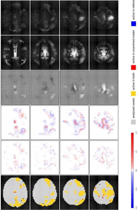
• log(LR) = (log(LRi)) is the log-likelihood ratio statistic map with
log(LRi) = Tlog(Si0/Si1), which is a measure for the amount of
acti-vation information contained in the fMRI data. It is directly available
from our algorithm via (9) and is an alternative to the SPM F-map.
• J= (Ji) is the EEG-based prior information map.
• ηˆEEG = (ˆαiJi) resp. ˆηEEG= (ˆαGJi) is the estimated EEG contribution
to the latent probit predictor. It visualizes the strength and location of mere EEG effects.
• Φˆdiff =
Φ(ˆηi,iMRFglob/f lex); 0,1)−Φ(ˆηi,iMRF0; 0,1)
is the marginal prior probability difference map. To enhance the understanding of these,
note the following: It holds that ˆp(γi = 1|Uj6=i,θ−U) = Φ(ˆηi; 0,1) for
each voxel i. Being based on the posterior estimate ˆηi of ηi = η0+
ηEEG, this quantity can be interpreted as an adaptive prior probability
for activation—taking into account the latent effects arising from the fMRI and EEG activation information, and the congruency of both. In
the figures, the difference maps visualize how the adaptive prior map changes when EEG information is incorporated.
• πˆdiff = ˆp(γi = 1|θ,y,iMRFglob/f lex)−pˆ(γi = 1|θ,y,iMRF0)
is the pos-terior activation probability difference map. Pospos-terior activation prob-ability maps are thresholded (cf. Sect. 2.5) to gain activation maps and, hence, visualize the EEG impact on a continuous level.
• γˆdiff = γˆi,iMRFglob/f lex −γˆi,iMRF0
is the categorical activation
differ-ence map between iMRFglob resp. iMRFf lex and iMRF0. The impact
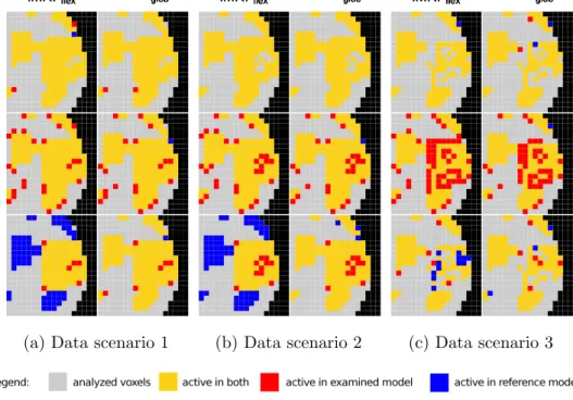
of incorporating EEG information can most easily be seen with this kind of map, where yellow indicates voxel found to be activated with both algorithms, red indicates voxels only found by the EEG enhance-ment and blue indicates voxels only found by the uninformed reference model.
In Fig. 1, the results of iMRFf lex are depicted. We select result maps
from brain slices 21, 23, 25 and 27, because these slices comprise the parts
of the brain where the EEG information is strong (compare J maps) and is
supposed to especially add value to the activation detection (compare low values in log(LR) maps).
For ˆηEEG, each Ji value is multiplied with a spatially-varying effect αi
to form ˆηEEG,i. We see, that ˆηEEG is zero (medium grey areas), if Ji = 0.
In other regions (with Ji > 0), deviations to negative (dark-grey) or
posi-tive (light-grey) values arise, because the spatially-varying effect αi is
non-restricted. If ˆαi< 0, then the EEG effect speaks for non-activation, if ˆαi>0,
otherwise. It appears that theαi-values depend on the grade of congruency
between EEG (J) and fMRI (log(LR)) information. The influence of ˆηEEG
can be compensated by the spatially-varying intercept. Both terms sum up
to form the whole predictor value ˆη. Structural effects on the whole predictor
level are examined via ˆΦdiff, which we discuss next.
Marginal prior probability difference maps ˆΦdiff can be used to assess the
latent predictor estimation. Here, we observe changes in predictor estimation mainly in parts of the brain where fMRI activation is present (non-white ar-eas). This hints at the stability of the algorithm, because predictor values are not changed in arbitrary parts of the brain. The marginal prior activation probability is especially increased at activation region boundaries, e.g. at the central activation focus in slices 25 and 27 (red-scale areas). In adjacent re-gions, the marginal prior probability of voxels is decreased (blue-scale areas),
c(0, 1) log
(
LR)
Slices 21 23 25 27 c(0, 1) J c(0, 1) η^ EEG c(0, 1) Φ^diff c(0, 1) π^ diff γ ^ diff c(0, 1) log(
LR)
Slices 21 23 25 27 c(0, 1) J c(0, 1) η^ EEG c(0, 1) Φ^diff c(0, 1) π^ diff γ ^ diffFigure 1: Summary of results from the iMRFf lex model in comparison to
c(0, 1) log
(
LR)
Slices 21 23 25 27 c(0, 1) J c(0, 1) η^ EEG c(0, 1) Φ^diff c(0, 1) π^ diff γ ^ diff c(0, 1) log(
LR)
Slices 21 23 25 27 c(0, 1) J c(0, 1) η^ EEG c(0, 1) Φ^diff c(0, 1) π^ diff γ ^ diffFigure 2: Summary of results from the iMRFglob model in comparison to
which indicates that EEG contradicts fMRI activation information there. That is, the EEG activation focus is not congruent to the fMRI activation focus: The EEG peak covers the fMRI peak, but it exceeds the fMRI peak
by far. That iMRFf lex detects these edges can be regarded as a feature of
the algorithm, because it indicates robustness against non-congruency of the EEG prior. In summary, on the one hand, when EEG information contradicts fMRI information, the EEG contribution seems to be either downweighted or to be used as information on deactivation. On the other hand, when EEG information is congruent to fMRI information, the EEG contribution is in-creased. Regarding the sharp boundaries between red- and blue-scale areas, the algorithm appears to possess good edge-preserving properties—which, however, may prevent EEG-enhancement (see Discussion).
So far, we see that marginal prior probability maps ˆΦdiff possess a
struc-turally sensible form of EEG dependency. Whether this is carried through to activation classifications can be deferred from posterior activation
probabil-ity maps ˆπdiff. The iMRFf lex algorithm locates largest posterior probability
differences at activation region boundaries. Posterior activation probabilities are either increased or decreased. Particularly, with supporting EEG infor-mation, i.e. in central parts of the brain, we observe an increase in posterior activation probabilities.
In ˆγdiff, we see that changes in posterior activation probabilities are large
enough to slightly increase region sizes in targeted areas (e.g. in the cen-tral part in layer 27). However, a few voxels also become non-active in regions where algorithms emphasize sharp edges between activation and non-activation zones.
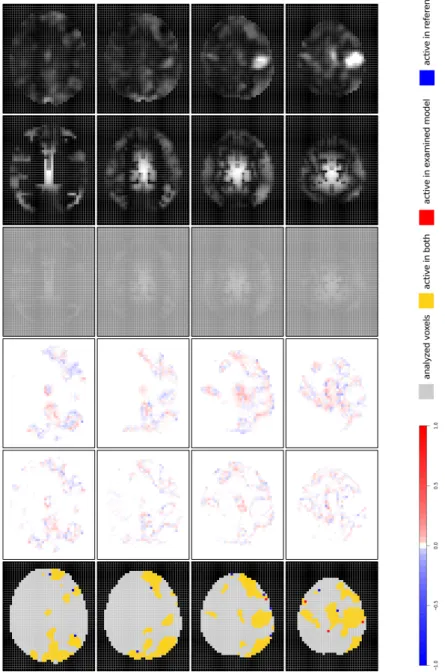
In Fig. 2, the results of the iMRFglob analysis can be found. For the ˆηEEG,
each Ji value is multiplied with a global effect αG to form ˆηEEG,i. We see
again, that ˆηEEGis zero (medium grey areas), ifJi = 0. In other regions (with
Ji >0), positive values arise (light-grey areas), because the global effectαGis
restricted to non-zero values. Note that the colour scale of the ˆηEEG-maps are
chosen with respect to the range of the whole predictor. Hence, if the EEG component is not sufficiently strong, the contrast of the image is low. This happens here, because a global EEG effect is calculated that poorly stands
out from the intercept component. Nevertheless, as it can be seen from ˆΦdiff
and ˆπdiff maps, it is strong enough to affect posterior activation probabilities.
However, due to its weakness it is not able to substantially increase sensitivity in this particular application. As soon as EEG contradicts fMRI in larger parts of the brain, the global EEG effect is estimated to be so small that it
hardly influences activation probability and, hence, activation classification (ˆγdiff).
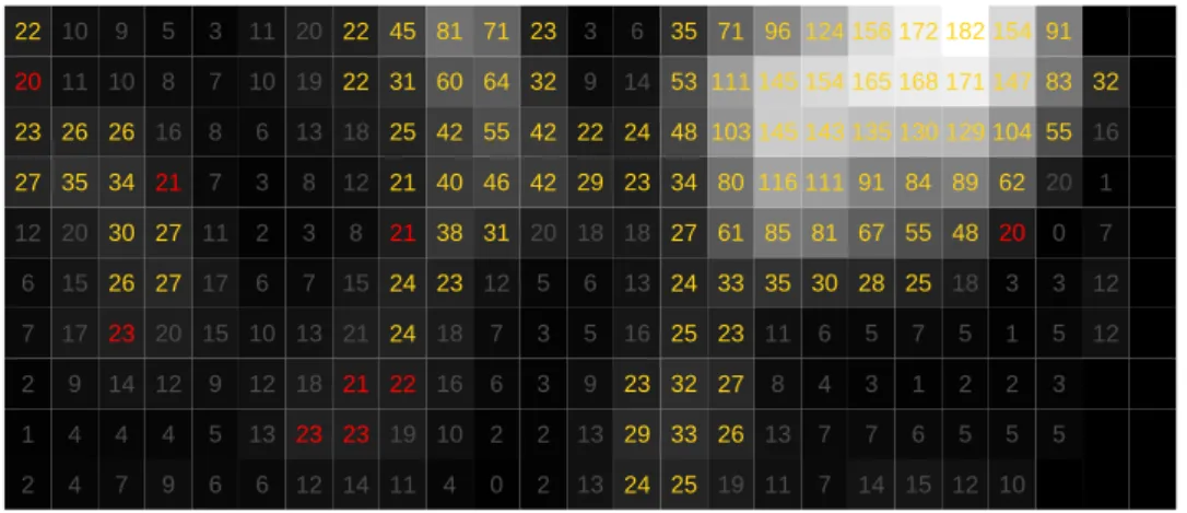
Thus, we have seen that the global and local degree of congruency has a strong effect on the performance of the EEG enhancement. To elaborate on this, in Fig. 3a, we visualized the overlap of EEG and fMRI information of a region of interest (center of slice 27). As before, voxelwise fMRI acti-vation information is provided through log(LR) statistics, whereas for EEG,
the correspondingJ-values are plotted. Additionally in Fig. 3b, the log(LR)
values are plotted, with the values being colour-coded as in the activation
difference maps—displaying the activation differences between iMRFf lexand
iMRFglob. From these plots, we see that the fMRI peaks are well-pronounced
and log(LR) values decrease to very small values in in-between activation regions. Only at region borders, there are some voxels with medium sized log(LR) values indicating that some amount of activation is contained in corresponding time series. Hence, the number of voxels, where the EEG information is supposed to enhance activation information, is limited. Ad-ditionally, from Fig. 3b, we see that the overlap between EEG and fMRI information is not sufficient to increase sensitivity of activation detection to a large extent. For example, a small cluster of four voxels can be forced to be found active, but not surrounding voxels with nearly as high log(LR)-values, because the EEG is not sufficiently strong in this region.
4. Simulation study
Although, iMRFf lex and iMRFglob models did only achieve a minor gain
in sensitivity in our particular application, analysis results gave rise for some assumptions about suitable data structures, where EEG-enhanced fMRI ac-tivation detection algorithms are expected to lead to a substantial gain in sensitivity. Assume that we have a ROI where EEG information should en-hance sensitivity in fMRI activation detection. We have, for example, seen that the EEG prior and fMRI data must be fairly congruent in this ROI and that the fMRI time series of corresponding voxels must contain a sufficient amount of activation information. Moreover, the ROI is preferably not just a border, but a de-noised peak structure. To yield some support for these assumptions, we set up the following simulation study based on modifications of the original dataset analysed in the previous section.
To decrease computation time, we took a subset of the data (with 3D
2 1 2 7 6 12 27 23 20 22 4 4 9 17 15 20 35 26 11 10 7 4 14 23 26 30 34 26 10 9 9 4 12 20 27 27 21 16 8 5 6 5 9 15 17 11 7 8 7 3 6 13 12 10 6 2 3 6 10 11 12 23 18 13 7 3 8 13 19 20 14 23 21 21 15 8 12 18 22 22 11 19 22 24 24 21 21 25 31 45 4 10 16 18 23 38 40 42 60 81 0 2 6 7 12 31 46 55 64 71 2 2 3 3 5 20 42 42 32 23 13 13 9 5 6 18 29 22 9 3 24 29 23 16 13 18 23 24 14 6 25 33 32 25 24 27 34 48 53 35 19 26 27 23 33 61 80 103 111 71 11 13 8 11 35 85 116 145 145 96 7 7 4 6 30 81 111 143 154 124 14 7 3 5 28 67 91 135 165 156 15 6 1 7 25 55 84 130 168 172 12 5 2 5 18 48 89 129 171 182 10 5 2 1 3 20 62 104 147 154 5 3 5 3 0 20 55 83 91 12 12 7 1 16 32
(a) Map with log(LR)-statistic information (grey-scale and numbers). Font colour indicates activation classification differences between iMRFf lex and iMRF0.
(b) Overlap of EEG (red-scale) and fMRI (grey-scale) information. Here: the higher the colour saturation, the higher activation information.
Figure 3: Informational content of combined EEG and fMRI dataset in the center of slice 27.
14 13 19 26 26 17 12 13 17 19 14 9 9 12 18 19 17 9 5 5 7 8 15 21 21 18 12 13 21 25 24 23 25 30 33 26 18 9 4 5 1 2 4 10 14 17 17 14 14 18 31 51 64 64 48 29 17 8 2 3 2 2 2 6 13 19 18 11 8 12 34 73 95 90 64 34 19 7 5 19 1 0 1 5 11 14 15 12 8 10 21 47 82 76 47 27 17 5 13 32 2 5 7 8 8 5 7 11 10 10 10 16 37 36 19 11 6 3 16 25 6 10 12 12 10 6 5 12 17 15 13 16 29 26 16 8 0 4 9 12 15 22 23 21 19 19 20 25 25 24 29 31 34 28 19 8 1 2 5 9 20 33 37 37 37 40 43 42 41 47 56 55 46 34 21 6 4 8 14 22 15 30 40 45 55 61 56 66 89 112 115 93 64 47 26 6 5 13 23 35 4 21 34 44 56 62 61 98 111 62 76 122 81 58 28 5 8 19 24 33 2 3 21 29 26 30 44 95 34 20 33 135 101 70 26 3 16 27 26 27 11 6 2 4 5 7 26 76 101 6 21 51 119 79 19 12 25 25 22 12 9 6 1 4 24 65 125 40 10 23 132 86 19 19 25 19 6 2 5 20 51 100 112 13 27 137 82 18 3 9 30 68 99 123 132
(a) Data scenario 1
14 13 19 26 26 17 12 13 17 19 14 9 9 12 18 19 17 9 5 5 7 8 15 21 21 18 12 13 21 25 24 23 25 30 33 26 18 9 4 5 1 2 4 10 14 17 17 14 14 18 31 51 64 64 48 29 17 8 2 3 2 2 2 6 13 19 18 11 8 12 34 73 95 90 64 34 19 7 5 19 1 0 1 5 11 14 15 12 8 10 21 47 82 76 47 27 17 5 13 32 2 5 7 8 8 5 7 11 10 10 10 16 37 36 19 11 6 3 16 25 6 10 12 12 10 6 5 12 17 15 13 16 29 26 16 8 0 4 9 12 15 22 23 21 19 19 21 26 25 25 26 29 35 27 19 8 1 2 5 9 20 33 37 37 37 41 44 43 41 46 51 44 44 33 20 6 4 8 14 22 15 30 40 45 55 53 43 45 62 53 46 51 72 46 25 6 5 13 23 35 4 21 34 44 56 50 56 36 28 22 21 29 52 51 26 5 8 19 24 33 2 3 21 29 26 29 42 55 9 21 13 32 35 59 25 3 16 27 26 27 11 6 2 4 5 7 27 66 11 11 28 8 36 57 19 12 25 25 22 12 9 6 1 4 24 49 22 32 13 17 42 72 19 19 25 19 6 2 5 20 53 53 34 13 25 34 62 18 3 9 30 60 47 30 29 (b) Data scenario 2 14 13 19 26 26 17 12 13 17 19 14 9 9 12 18 19 17 9 5 5 7 8 15 21 21 18 12 13 21 25 24 23 25 30 33 26 18 9 4 5 1 2 4 10 14 17 17 14 14 18 31 51 64 64 48 29 17 8 2 3 2 2 2 6 13 19 18 11 8 12 34 73 95 90 64 34 19 7 5 19 1 0 1 5 11 14 15 12 8 10 21 47 82 76 47 27 17 5 13 32 2 5 7 8 8 5 7 11 10 10 10 16 37 36 19 11 6 3 16 25 6 10 12 12 10 6 5 12 17 15 13 16 29 26 16 8 0 4 9 12 15 22 23 21 19 10 19 21 10 24 5 6 22 12 16 8 1 2 5 9 20 33 37 37 37 22 26 24 24 17 20 9 16 14 6 6 4 8 14 22 15 30 40 45 55 18 10 10 33 34 29 21 48 23 8 6 5 13 23 35 4 21 34 44 56 18 26 14 27 25 24 17 18 21 9 5 8 19 24 33 2 3 21 29 26 11 20 29 12 29 17 25 14 25 12 3 16 27 26 27 11 6 2 4 5 6 18 33 10 20 40 10 23 25 12 12 25 25 22 12 9 6 1 7 14 16 14 40 19 23 33 37 8 19 25 19 6 2 1 12 30 27 34 20 33 28 28 16 6 5 15 27 23 17 25 (c) Data scenario 3
Figure 4: Simulation scenarios: Activation information contained in fMRI data.
(neurologically) right part of Brodmann areas 1-4, 6 (containing the primary somatosensory, primary motor and premotor cortex), which showed a strong fMRI signal in prior analyses. Since the original data structure possessed well pronounced, smooth activation peaks, we decided to de-noise the observed peak structure. For this, we used three different strategies (cf. Fig. 4). Data scenario 1 was generated to contain a hole within the activation structure with surrounding strongly activated voxels. Data scenario 2 was generated to contain a slightly larger hole, but surrounding voxels were forced to ob-tain much smaller log(LR) values than in scenario 1. In data scenario 3, the whole activation region was distorted by noise. As artificial prior EEG information, we used two congruent information maps in form of the binary
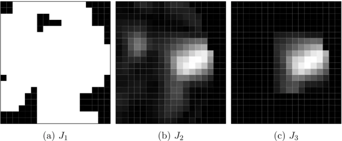
extended fMRI activation map (denoted as J1, cf. Fig. 5a) and in form of
the continuous log(LR)-map (denoted as J2, cf. Fig. 5b) from the original
dataset without additional noise. As a form of local prior information, we additionally used the log(LR) map that was set to zero outside a rectangular
region of 8×9 voxels covering the targeted activation focus across all slices
(denoted as J3, cf. Fig. 5c). This prior introduced non-congruency in large
parts of the analysed brain, whereupon non-congruent regions adjoined the targeted activation focus with congruent information at some borders.
In Fig. 6, the results in form of activation difference maps in reference to
iMRF0 are given. Each two-column block depicts the results from the three
(a) J1 (b) J2 (c) J3
Figure 5: Simulation scenarios: Different types of EEG prior information
based on the non-denoised data. Prior J1 is the underlying activation map
from an initial run. PriorJ2 is a congruent, continuous prior in form of the
underlying log(LR)-map. Prior J3 is a non-congruent, continuous prior in
form of a cut log(LR)-map.
prior types are presented in each row.
With J1, some voxels at the borders of the activation region change their
state, but no changes occur in the targeted region inside the activation focus. Particularly, no sensitivity increase is achieved. Hence, we conclude that if the EEG-prior information is not strong enough, EEG-enhanced activation schemes cannot make use of it.
WithJ2, iMRFf lexand iMRFglob perform very well compensating the lost
activation in any case. Note that the iMRF algorithms incline to smooth across region edges enlarging peak regions as well.
With J3, iMRFglob performs well in data scenarios 1 and 2, but it
can-not compensate the loss in data scenario 3—indicating that if the activation structure is too de-noised, non-congruent EEG information cannot compen-sate the loss. This might be traced back to the fact that in the non-congruent setting at hand, there is not enough information in the data to achieve a
suffi-ciently large global EEG effect estimate. In contrast to this, iMRFf lexindeed
compensate the loss in data scenarios 1 and 2, but outside the activation
fo-cus, all voxels become non-activated. This might indicate that iMRFf lexuses
EEG prior information also on non-activation. If peak structures are too
deteriorates the activation structure.
5. Discussion
In this work, we proposed a novel strategy for the fMRI-EEG data fusion— unequal to any fusion approach found in the literature. We extended the Bayesian fMRI activation detection approach from Smith et al. (2003) to incorporate spatial EEG information in form of 3D prior activation infor-mation to enhance sensitivity. More precisely, a high-dimensional Bayesian variable selection approach was used to relate spatial EEG-prior information to voxelwise selection probabilities of a global stimulus regressor component. These probabilities were then used as indicators for activation, i.e. as ac-tivation probabilities. Continuous or binary EEG information was thereby connected to activation probabilities by using a latent probit regression stage. The probit predictor was chosen to consist of at least one spatially-varying effect (intercept or EEG component or both) to adapt to local brain re-sponse. Spatially-varying effects were regularized by an intrinsic Gaussian Markov random field (IGMRF) prior to ensure identifiability of voxelwise effects and to impose a dependency structure on neighbouring voxels. Re-sults from a Gaussian conditional autoregressive (CAR) prior can be found in Kalus (2012). Inference was based on a Markov chain Monte Carlo (MCMC)
sampling scheme. Two algorithms, iMRFglob and iMRFf lex, were proposed,
which differ in the way how they incorporate EEG information. Their perfor-mance was examined in reference to an activation detection scheme without
EEG-enhancement (iMRF0).
In case of iMRFf lex, an spatially-varying EEG coefficient regulates the
EEG influence on activation detection and adapts it to local conditions. That is, it increases EEG influence in brain parts where EEG and fMRI are in accordance with each other and downweights EEG influence where it contradicts the fMRI signal. This implicates that the algorithm is quite robust against misspecifications in EEG-prior choice. In Sect. 4, we have
also seen that iMRFf lex might use non-congruent prior information as
in-formation on non-activation. This finding, however, has to be corroborated in further studies. Generally, a requirement for increasing sensitivity in re-gions of special interest seems to be that these are not too close to rere-gions with non-overlapping fMRI and EEG information. If these areas are dis-tant enough, the downweighting mechanism, which is related to good edge-preserving properties, does not interfere with the positive EEG influence in
J1
J2
J3
iMRFflex iMRFglob
J1
J2
J3
iMRFflex iMRFglob
J1
J2
J3
iMRFflex iMRFglob
J1
J2
J3
iMRFflex iMRFglob
J1
J2
J3
iMRFflex iMRFglob
J1
J2
J3
iMRFflex iMRFglob
(a) Data scenario 1
J1
J2
J3
iMRFflex iMRFglob
J1
J2
J3
iMRFflex iMRFglob
J1
J2
J3
iMRFflex iMRFglob
(b) Data scenario 2
J1
J2
J3
iMRFflex iMRFglob
J1
J2
J3
iMRFflex iMRFglob
J1
J2
J3
iMRFflex iMRFglob
(c) Data scenario 3
Figure 6: Simulation results: Activation difference maps of iMRFf lex resp.
other regions. Thereby, the corresponding minimal distance depends on the degree of smoothness in the data and is likely to span only a small number of voxels. To assess congruency, EEG effect map estimates can give information about the overlap of fMRI and EEG data and, hence, give hints on possible problems.
In case of iMRFglob, the global EEG effect possesses the ability to increase
prior activation probabilities proportionally to the observed EEG measure-ments as soon as a reasonable large, positive EEG effect is retrieved. If neces-sary, the spatially-varying intercept can have a region-specific compensating effect to improve the goodness-of-fit. The size of the EEG effect depends on the degree of congruency of fMRI and EEG data. If EEG information does not match fMRI information in large parts of the analysed brain, a virtually zero global EEG effect estimate is recovered. Hence, this algorithm
is equally robust against misspecifications, but, in contrast to iMRFf lex, it
loses its ability to increase sensitivity in remaining congruent areas.
Comparing the performance of both predictor types, we generally expect
that iMRFf lex models possess a better performance than iMRFglob models
when non-congruency is present in the data. The iMRFglob algorithm
re-trieves a global EEG effect by averaging over all analysed brain parts, so that the effect may be decreased (even to virtually zero estimates) if too
much non-congruency is in the data. In contrast to this, iMRFf lex is able to
adapt the EEG effect to local conditions. As long as regions are sufficiently separated, effects in non-congruent areas do not substantially influence effects in congruent areas, which can retain their high sensitivity level. Generally, we observed that both algorithms are approximately as sensitive as their
cor-responding uninformed fMRI activation detection algorithm iMRF0 in most
analyses.
Indeed, iMRFglob and iMRFf lex had a promising performance, because
they appeared to recover interpretable estimates by retaining the high
sen-sitivity level of iMRF0. However, despite our expectations, EEG-enhanced
fMRI activation detection schemes only revealed their benefit in data set-tings with certain properties. From these findings, we suppose that they are useful in regions where fMRI data possess activation structures of reasonable large size (not just isolated peaks) with gaps in the structure (e.g. due to noise). Within this region, non-active voxels containing a damped activation signal can then be classified as active if prior information—in form of suf-ficiently strong EEG measurements—indicates activation at these locations. Thereby the prior information must be fairly congruent to fMRI activation
information overall the analysed brain.
In our real-world example, the data structure deviated from these guide-lines. Therefore, only a relatively small number of voxels switched their status from being non-active to active. Hence, we saw indeed that our EEG enhancement possesses some potential to increase sensitivity, but in this par-ticular application, it had not lived up to expectations. In controlled settings, like in the simulation study, we observed, however, a substantial performance increase with data that possessed the above properties.
We conclude with some remarks on current or future research: The as-sumption of independent error terms might be relaxed by incorporating tem-poral correlations in voxelwise fMRI regressions. We do not expect that the performance of proposed algorithms is strongly influenced by this, but a more realistic model might be achieved through this. Marginalization steps to fMRI regression parameters, however, might not be feasible anymore— leading to a far inefficient sampling procedure.
Incorporation of brain partitioning information is of particular interest (see, for example, the description in Appendix B of Daunizeau et al., 2007). Estimation of random fields and corresponding variance parameters then could be broken down into parts and be accomplished within (more) ho-mogeneous brain areas. This would be advantageous in several ways: The speed of the algorithms could be increased, smoothness of random field may
be allowed to vary across the brain and for iMRFglob non-congruency issues
(leading to small global EEG effect estimates) can be resolved by this as well. The existing approaches can further be modified by changing the fitting algorithm. Though the full Bayesian MCMC approach finds the exact poste-rior distribution of model parameters, it is rather slow. Another popular ap-proach in neuroimaging is a variational Bayes apap-proach to Bayesian inference (see e.g. Titterington, 2004). It approximates the joint posterior distribution of all unknown parameters with a simpler distribution usually positing fur-ther independence assumptions than those implied by the original generative model. By this, the computational demand can be decreased substantially. However, a comparison between full and approximate Bayesian approaches has to be conducted to check whether the speed is achieved at the expense of accuracy.
Note that in this work, we focussed on modelling activation provoked by just one stimulus type. Nevertheless, it is conceivable that other stimulus types, which are presented within the same experimental procedure, are ei-ther included as confounders or as a furei-ther additive stimulus component
that is subject to Bayesian activation detection. Generally, our methodol-ogy is not applicable to stimulus-free experimental procedures like resting state observations. For being inevitably connected to a regressor modelling some kind of stimulus that provokes neuronal activation, an extension to stimulus-free settings is not conceivable.
As noted above, the EEG-enhanced activation detection schemes have not lived up to our expectations in the application at hand. Nevertheless, in the
simulation study iMRFf lex and iMRFglob yielded promising results. Hence,
demonstrating their potential in other data settings, with suitable structure and carefully selected 3D prior knowledge (either derived from EEG or other external information), will be of great interest.
6. Acknowledgements
We are grateful to Sara A. Kiem for supporting data acquisition of the acoustic oddball paradigm, and Manuela H¨olzwimmer and Ludwig Both-mann for assisting the EEG source localization process. This research has been funded by the German Science Foundation, grant FA 128/6-1.
References
Albert, J.H., Chib, S., 1993. Bayesian analysis of binary and polychotomous response data. J Am Stat Assoc 88, 669–679.
Bandettini, P.A., 2012. 20 years of fMRI [Special issue]. NeuroImage 62, 575–1324.
Barbieri, M.M., Berger, J.O., 2004. Optimal predictive model selection. The Annals of Statistics 32, 870–897.
Beckmann, C.F., Smith, S.M., 2005. Tensorial extensions of independent component analysis for multisubject FMRI analysis. NeuroImage 25, 294– 311.
Czisch, M., Wehrle, R., Stiegler, A., Peters, H., Andrade, K., Holsboer, F., S¨amann, P.G., 2009. Acoustic oddball during NREM sleep: a combined EEG/fMRI study. PLoS ONE 4, e6749.