2010
Representing and reasoning with qualitative
preferences for compositional systems
Ganesh Ram Santhanam
Iowa State UniversityFollow this and additional works at:https://lib.dr.iastate.edu/etd Part of theComputer Sciences Commons
This Dissertation is brought to you for free and open access by the Iowa State University Capstones, Theses and Dissertations at Iowa State University Digital Repository. It has been accepted for inclusion in Graduate Theses and Dissertations by an authorized administrator of Iowa State University Digital Repository. For more information, please [email protected].
Recommended Citation
Santhanam, Ganesh Ram, "Representing and reasoning with qualitative preferences for compositional systems" (2010).Graduate Theses and Dissertations. 11834.
by
Ganesh Ram Santhanam
A dissertation submitted to the graduate faculty in partial fulfillment of the requirements for the degree of
DOCTOR OF PHILOSOPHY
Major: Computer Science Program of Study Committee: Vasant G. Honavar, Major Professor
Samik Basu Carl Chang Robyn Lutz Giora Slutzki
Iowa State University Ames, Iowa
2010
DEDICATION
TABLE OF CONTENTS
LIST OF TABLES . . . vii
LIST OF FIGURES . . . ix ACKNOWLEDGEMENTS . . . xii ABSTRACT . . . xiii CHAPTER 1. Introduction . . . 1 1.1 Contributions . . . 3 1.1.1 Dominance Testing . . . 3
1.1.2 Preference Reasoning for Compositional Systems . . . 4
1.1.3 Application of Preference Reasoning for Compositional Systems: Web services . . . 9
CHAPTER 2. Preliminaries . . . 12
2.1 Properties of Binary Relations . . . 12
2.2 Qualitative Preferences . . . 12
2.2.1 Qualitative Preference Languages . . . 14
2.2.2 Representing Qualitative Preferences: CP-nets and TCP-nets . . 15
2.2.3 Reasoning with Qualitative Preferences: Ceteris Paribus Semantics 17 2.2.4 Dominance Testing . . . 17
2.3 Compositional Systems . . . 19
2.3.1 Functional Composition . . . 20
CHAPTER 3. Efficient Preference Reasoning Techniques . . . 24
3.1 Efficient Dominance Testing for Unconditional Preferences . . . 24
3.1.1 A Language for Unconditional Preferences . . . 24
3.1.2 Dominance Testing forLT U P . . . 25
3.1.3 Semantics: Relationship Between ≻◦, ≻w &≻• . . . . 33
3.1.4 Concluding Remarks . . . 36
3.2 Dominance Testing via Model Checking . . . 37
3.2.1 Dominance Testing via Model Checking . . . 38
3.2.2 Kripke Structure Encoding of TCP-net Preferences . . . 40
3.2.3 Summary and Discussion . . . 46
CHAPTER 4. Preference Reasoning for Compositional Systems: The-ory & Algorithms . . . 49
4.1 Preference Formalism . . . 49
4.1.1 Aggregating Attribute Valuations across Components . . . 50
4.1.2 Comparing Aggregated Valuations . . . 54
4.1.3 Dominance: Preference over Compositions . . . 56
4.1.4 Choosing the Most Preferred Solutions . . . 62
4.2 Algorithms for Computing the Most Preferred Compositions . . . 63
4.2.1 Computing the Maximal/Minimal Subset with respect to a Partial Order . . . 63
4.2.2 Algorithms for Finding the Most Preferred Feasible Compositions 64 4.2.3 A Sound and Weakly Complete Algorithm . . . 65
4.2.4 Optimizing with Respect to One of the Most Important Attributes 69 4.2.5 Interleaving Functional Composition with Preferential Optimization 70 4.2.6 Complexity . . . 77
4.3.1 TCP-nets . . . 82
4.3.2 Preferences over Collections of Objects . . . 84
4.3.3 Database Preference Queries . . . 87
4.4 Summary . . . 89
4.5 Discussion . . . 91
CHAPTER 5. Preference Reasoning for Compositional Systems: Ex-periments & Results . . . 94
5.1 Experimental Setup . . . 94
5.1.1 Modeling the Search Space of Compositions using Recursive Trees 94 5.1.2 Implementation of Algorithms . . . 96
5.2 Results . . . 98
5.3 Analysis of Experimental Results . . . 107
5.4 Summary and Discussion . . . 114
CHAPTER 6. Preference Reasoning for Compositional Systems: Ap-plications to Web Services . . . 116
6.1 Service-oriented Systems as Compositional Systems . . . 116
6.2 Web Service Composition . . . 117
6.2.1 Background . . . 117
6.2.2 Problem Specification . . . 120
6.2.3 Utilizing TCP-nets in Web service composition . . . 124
6.2.4 TCP-Compose⋆ . . . 125
6.2.5 Summary and Discussion . . . 131
6.3 Web Service Substitution . . . 133
6.3.1 Preference Reasoning for Web Service Substitution . . . 138
6.3.2 Computing Preferred Substitutions . . . 140
6.3.4 Finding Preferred Order . . . 146
6.3.5 Summary and Discussion . . . 150
6.4 Web Service Adaptation . . . 151
6.4.1 Service Adaptation via Service Substitution . . . 154
6.4.2 Computing Preferred Adaptations . . . 156
6.4.3 A Sound Adaptation Algorithm . . . 159
6.4.4 Properties of AttributeAdapt . . . 160
6.4.5 A Sound and Weakly Complete Algorithm . . . 162
6.4.6 Properties of ExhaustiveAdapt . . . 164
6.4.7 Efficiency of ExhaustiveAdapt . . . 165
6.4.8 Summary and Discussion . . . 166
6.5 Discussion . . . 168
CHAPTER 7. Conclusion . . . 170
7.1 Contributions . . . 171
LIST OF TABLES
1.1 List of courses the student can choose from . . . 5
2.1 Properties of binary relations . . . 13
2.2 Notation . . . 23
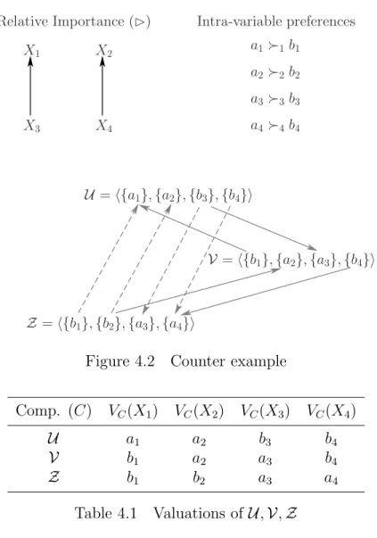
4.1 Valuations of U,V,Z . . . 60
4.2 Properties of ≻d for which the algorithms are sound, weakly complete and complete. po stands for partial order;io stands for interval order; wo stands for weak order; and |I| = 1 is when there is a unique most important attribute. . . 77
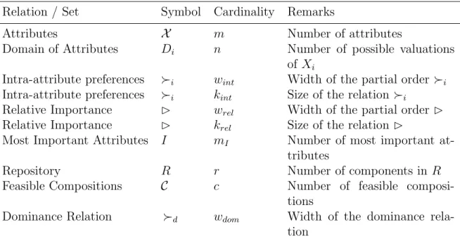
4.3 Cardinalities of sets and relations . . . 78
4.4 Properties/Attributes describing the senators . . . 86
5.1 Simulation parameters and their ranges . . . 97
5.2 Implemented Algorithms . . . 98
5.3 Attributes observed during the execution of each algorithm . . . 99
5.4 Comparison of SP/P F for algorithms A3 and A4 with respect to various ordering restrictions on{≻i},. The percent of prob-lem instances for which SP/P F = 1 is shown in each row with respect to the corresponding ordering restrictions on the prefer-ence relations and {≻i}. Plots from simulation experiments are shown in Figures 5.1 and 5.2. . . 100
5.5 Comparison of SP/S for algorithms A3 and A4 with respect to various ordering restrictions on{≻i},. The percent of problem instances for which SP/S = 1 is shown in each row with respect to the corresponding ordering restrictions on the preference rela-tions and {≻i}. Plots from simulation experiments are shown
in Figures 5.1 and 5.2. . . 101
5.6 Summary of results and conjectures relating to the properties of ≻d with respect to the properties of and { ≻′i}. . . 114
6.1 Domain Definition . . . 121
6.2 Preference Valuations . . . 141
6.3 Valuations of replacements . . . 144
6.4 Components . . . 156
LIST OF FIGURES
1.1 Intra-attribute preferences for Area (≻A) and Instructor (≻I). . 6
2.1 Example of a TCP-net with 3 binary variables, namelyA,B and C. It encodes the fact that the preference over values ofB andC are dependent on the value assigned to the variable A, and that it is relatively more important to have a preferred valuation for the variable B in comparison to having a preferred valuation for C. The intra-attribute preferences are given in the boxes next to the variables. . . 16
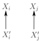
3.1 XiXj∧(XkXi∨Xk ∼ Xi) . . . 27
3.2 Xi ∼ Xj . . . 28
3.3 A 2⊕2 substructure, not an Interval Order . . . 32
3.4 (a) TCP-netN; (b) Transitive Reduction of δ(N) . . . 39
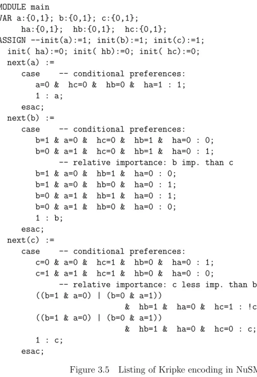
3.5 Listing of Kripke encoding in NuSMV . . . 48
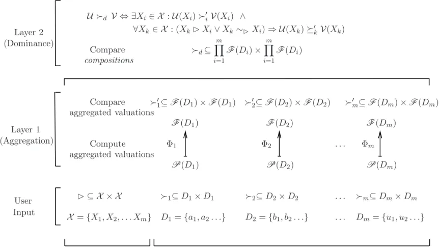
4.1 Dominance: Preference over compositions . . . 57
4.2 Counter example . . . 60
4.3 Intra-attribute preference ≻1 for attribute X1 . . . 73
4.4 Execution of Algorithm 4 . . . 73
4.6 Dominance relationships that violate the interval order
restric-tion on ≻d . . . 75
5.1 A comparison of the algorithmsA3 andA4 with respect toSP/P F and SP/S. . . 102
5.2 A comparison of the algorithmsA3 andA4 with respect toSP/P F and SP/S. . . 103
5.3 Number of invocations of functional composition algorithm for A1,A3 and A4 when f eas= 0.25,0.5,0.75,1.0. . . 105
5.4 Running times of algorithmsA1,A3 andA4 with 10 milliseconds per functional composition step for f eas= 0.25,0.5,0.75,1.0. . . 108
5.5 Running times of algorithms A1, A3 and A4 with 1000 millisec-onds per functional composition step forf eas= 0.25,0.5,0.75,1.0 . . . 109
5.6 The case when XpXq . . . 112
6.1 Goal Service . . . 120
6.2 Example CP-net and TCP-net . . . 122
6.3 Search Space for TCP-Compose⋆ when the TCP-net does not in-duce a total order over the set of valuations . . . 126
6.4 TCP-net: Representing Preferences and Importance . . . 137
6.5 Preferences: Multiple Component Substitution . . . 145
6.6 Multiple Component Substitution . . . 146
6.8 Number of subsets S ⊆ WC explored by ExhaustiveAdapt (z-axis) as a function of m (number of δis; the x-axis) and d (size of each δi; the y-axis). The plot is shown for c = 10 (number of components in WC). We observed similar trends for plots for c= 20,30. . .100. . . 167
ACKNOWLEDGEMENTS
I am very grateful to Dr. Honavar for first of all suggesting to me the idea of pursuing a PhD, and for his valuable guidance throughout. I am thankful for the freedom he gave me to explore research directions of my choice. I am also very grateful to Dr. Basu for giving his valuable time and for enthusiastically evaluating my research ideas. I am grateful to the other members of my committee for giving their valuable time and inputs. I am thankful to Bhavesh for his kind and friendly association, and the other AI lab members. I thank all the departmental staff for their timely help. I gratefully acknowledge the support I received from Dr. Honavar, Dr. Basu and Dr. McCalley through the NSF grants CNS0709217, CCF0702758, IIS0711356 and CNS0540293.
I am deeply indebted to Dr. P.V.Krishnan, who taught me that education should be aimed at developing perfect character. I am very grateful to Dr. Rangan and many other friends for their loving association during the program, which helped me make steady progress in my PhD and in all other aspects of life.
I am extremely grateful to my parents and family members for allowing me to pursue this program, and for their support and encouragement throughout.
ABSTRACT
Many applications call for techniques for representing and reasoning about prefer-ences, i.e., relative desirability over a set of alternatives. Preferences over the alternatives are typically derived from preferences with respect to the various attributes of the al-ternatives (e.g., a student’s preference for one course over another may be influenced by his preference for the topic, the time of the day when the course is offered, etc.). Such preferences are often qualitative and conditional. When the alternatives are expressed as tuples of valuations of the relevant attributes, preferences between alternatives can often be expressed in the form of (a) preferences over the values of each attribute, and (b) relative importance of certain attributes over others. An important problem in rea-soning with multi-attribute qualitative preferences is dominance testing, i.e., to find if one alternative (assignment to all attributes) is preferred over another. This problem is hard (PSPACE-complete) in general for well known qualitative conditional preference languages such as TCP-nets.
We provide two practical approaches to dominance testing. First, we study a re-stricted unconditional preference language, and provide a dominance relation that can be computed in polynomial time by evaluating the satisfiability of an appropriately con-structed logic formula. Second, we show how to reduce dominance testing for TCP-nets to reachability analysis in aninduced preference graph. We provide an encoding of TCP-nets in the form of a Kripke structure for CTL. We show how to compute dominance using NuSMV, a model checker for CTL.
outcomes or alternatives to be compared are composite in nature (i.e., collections of com-ponents that satisfy certain functional requirements). We define a dominance relation that allows us to compare collections of objects in terms of preferences over attributes of the objects that make up the collection, and show that the dominance relation is a strict partial order under certain conditions. We provide algorithms that use this dominance relation to identify only (sound), all (complete), or at least one (weakly complete) of the most preferred collections. We establish some key properties of the dominance relation and analyze the quality of solutions produced by the algorithms. We present results of simulation experiments aimed at comparing the algorithms, and report interesting conjectures and results that were derived from our analysis.
Finally, we show how the above formalism and algorithms can be used in preference-based service composition, substitution, and adaptation.
CHAPTER 1.
Introduction
Many applications call for techniques for representing and reasoning about pref-erences over a set of alternatives or outcomes. Such prefpref-erences may be qualitative
or quantitative. Qualitative preferences are expressed in the form of binary relations
(preference structures) on the set of alternatives, whereas quantitative preferences are expressed in the form of real valued functions on the set of alternatives.
Much of the work on decision theory has focused on reasoning with quantitative preferences [Fishburn, 1970, Keeney and Raiffa, 1993]. Value theory provides tools for encoding quantitative preferences using a value function, which assigns a value to each alternative. If v is a value function on the set {A, B, C} of alternatives, then A is said to be preferred to B if and only if v(A) > v(B). Utility functions have further been developed as an extension of value functions to deal with settings where the outcomes are uncertain (e.g., by incorporating a probability distribution over the set of outcomes). However, in many settings quantitative preferences may not exist, or it may be more natural to express preferences in qualitative terms [Doyle and Thomason, 1999]. Hence, there is a growing interest on formalisms for representing and reasoning with qualitative preferences [Brafman and Domshlak, 2009] in AI.
An important problem in this context has to do with representing qualitative prefer-ences over a set of alternatives, and reasoning with them to identify the most preferred ones. Typically, the alternatives are described by a set of attributes, and preferences over the alternatives are expressed with respect to their attributes. Representing and reasoning with preferences over multiple attributes is complicated by the fact that there
is an exponential increase in the number of possible outcomes over which preferences have to be specified. This brings the need for formalisms that compactly represent such preferences, and algorithms that reason with them.
Brafman’s seminal work [Brafman et al., 2006] attempts to address this need by introducingpreference networks, which are graphical formalisms for compactly encoding preferences over multiple attributes in the form of: (a) intra-variable or intra-attribute preferences specifying preferences over the domains of each of the attributes; (b) the
relative importanceamong the attributes. They can capture conditional preferences, i.e.,
preferences that arise in settings where the preferences over the values of an attribute is dependent on the assignment to one or more other attributes. Preference networks use a graphical representation scheme to encode the above types of preferences, and employ
the ceteris paribus1 semantics to reason about the most preferred alternatives. Two
of the well studied formalisms in this family are the conditional preference networks (CP-nets) that capture intra-attribute preferences, and tradeoff-enhanced conditional preference networks (TCP-nets) that capture intra-attribute preferences and relative importance over the attributes.
Against the above background, this thesis makes contributions in three related topics: 1. Dominance testing: Determining whether an outcome is preferred to another with respect to a set of preferences specified by a TCP-net is computationally hard. This thesis provides formal methods for performing dominance testing efficiently in many practical cases.
2. Preference Reasoning for Compositional Systems: In many AI applica-tions such as planning and scheduling, the alternatives over which preferences are computed represent collections of objects rather than simple objects. This thesis develops formalisms to reason with preferences over collections of objects based
on the preferences over the attributes of the objects that make up the collections, and provides algorithms to compute the most preferred collections.
3. Application to Web Services: The service oriented computing paradigm offers a powerful approach for software development, where independently developed distributed software components called Web services are assembled together to build more complex applications or compositions. This thesis provides algorithms for automatically identifying, repairing and adapting compositions satisfying a given requirement that are also most preferred with respect to the preferences over the set of attributes.
1.1
Contributions
We describe the specific research challenges, objectives and the contributions made in this thesis in relation to the above topics in Sections 1.1.1, 1.1.2 and 1.1.3 respectively.
1.1.1 Dominance Testing
A problem of fundamental importance in reasoning with qualitative preferences over multiple attributes is dominance testing. Dominance testing is the problem of deter-mining whether an outcome (an assignment to all the attributes) is preferred to another with respect to a given set of preferences. In languages such as CP-nets and TCP-nets, testing whether an outcome α is preferred to another outcome β with respect to a set of preferences is equivalent to finding a path in the graph of all possible outcomes from α to β [Brafman et al., 2006].
Polynomial algorithms exist for very special cases of CP-nets (such as when the dependencies of the attributes in a CP-net form a tree structure [Boutilier et al., 2004]).
However, the problem in the general case is hard (PSPACE-complete, [Goldsmith et al., 2008]). Hence, there is a need for practical algorithms for dominance testing.
Experience with other hard problems such as boolean satisfiability (SAT) suggests that many instances of the hard problem may be easily solvable. Specialized data struc-tures and algorithms have thus been developed to obtain practically useful tools (i.e., SAT solvers).
The first main contribution of this thesis is to address the practical need for efficient dominance testing methods for preference languages such as CP-nets and TCP-nets. In particular, we (a) study a restricted preference language for which dominance testing is polynomial time solvable; and (b) employ the state-of-the-art tools in formal methods to make the search for a proof of dominance efficient. This allows us to leverage continuing advances in model checking for more efficient preference reasoning.
1.1.2 Preference Reasoning for Compositional Systems
In many AI applications such as planning and scheduling, the alternatives over which preferences are computed have a composite structure, i.e., an alternative represents a collection or a composition of objects rather than simple objects. In such settings, typically there are a set of user specified functional requirements that compositions are required to satisfy2. Among all the possible compositions that do satisfy the functional requirements, there is often a need to choose compositions that are most preferred with respect to a set of user preferences. In particular, we are interested in the setting where the user preferences are specified with respect to a set of non-functional attributes of the objects that make up the composition. We illustrate the above problem using the following example.
Consider the task of designing a program of study (POS) for a Masters student in the
2For example, in planning, a valid plan is a collection of actions that satisfies the goal; and in
scheduling, a valid schedule is a collection of task-to-resource assignments that respects the precedence constraints.
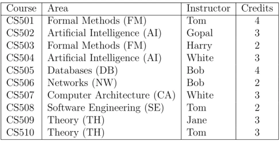
Computer Science department. The POS consists of a collection of courses chosen from a given repository of available courses spanning across different areas of focus in computer science. Apart from the area of focus, each course also has an assigned instructor and a number of credit hours. A repository of available courses, their areas of focus, their instructors and the number of credit hours are specified in Table 1.1.
Course Area Instructor Credits
CS501 Formal Methods (FM) Tom 4
CS502 Artificial Intelligence (AI) Gopal 3
CS503 Formal Methods (FM) Harry 2
CS504 Artificial Intelligence (AI) White 3
CS505 Databases (DB) Bob 4
CS506 Networks (NW) Bob 2
CS507 Computer Architecture (CA) White 3
CS508 Software Engineering (SE) Tom 2
CS509 Theory (TH) Jane 3
CS510 Theory (TH) Tom 3
Table 1.1 List of courses the student can choose from
In this example, each POS can be viewed as a composition of courses. The require-ments for an acceptable Masters POS (i.e., a feasible composition) are as follows.
• The POS should include at least 15 credits
• The POS should include the two core courses CS509 and CS510
• There should be courses covering at least two breadth areas of study (apart from the area of Theory (TH))
Given the repository of courses (Table 1.1), there may be one or more acceptable programs of study (i.e., feasible compositions). For example:
• P1 =CS501⊕CS502⊕CS503⊕CS504⊕CS509⊕CS510
F M T H AI DB N W SE CA (a) ≻A Jane Gopal Bob W hite Harry T om (b) ≻I
Figure 1.1 Intra-attribute preferences for Area (≻A) and Instructor (≻I). • P3 =CS503⊕CS504⊕CS507⊕CS508⊕CS509⊕CS510
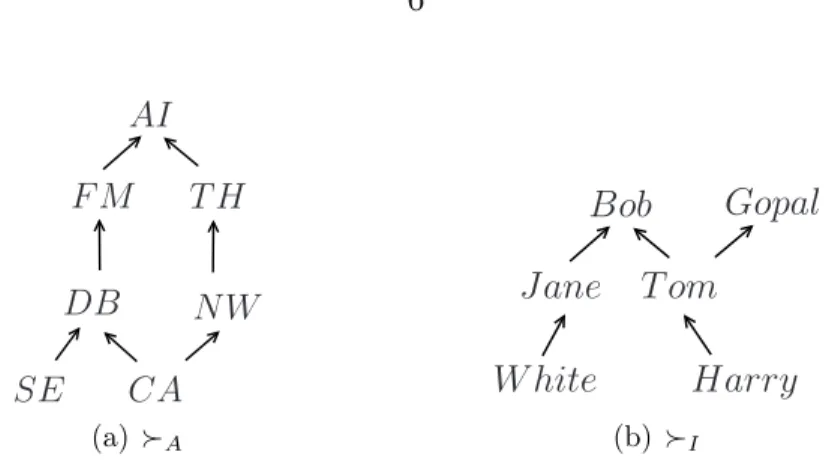
Suppose that in addition to the above requirements, a student has some preferences over the course attributes such as the area of focus, the choice of instructors and difficulty level in terms of credit hours. Among several acceptable programs of study, the student may be interested in those programs of study that: (a) satisfy the minimum requirements (see above) for an acceptable POS, and (b) those that are most preferred with respect to his/her preferences specified above. The preferences of a student with respect to the course attributes Area (A) and Instructor (I) are illustrated in Figure 1.1. In addition let us say that the student prefers the POS that have lesser total number of credits (this specifies ≻C). Further, let the relative importance among the attributes A, I and C be IAC3, i.e., I is relatively more important thanA, which is in turn relatively more important than C. Such preferences can be represented using TCP-nets.
The problems that we try to address in our research, given such a compositional system are:
• Given two programs of study, namely Pi and Pj, determine whether Pi≻dPj or vice versa with respect to the student’s preferences;
• Given a repository of courses and an algorithm for computing a set of acceptable
3
programs of study, find the most preferred, acceptable programs of study with respect to the above dominance relation.
In this example, the functional requirements correspond to the three conditions4, all of which must be satisfied for a collection of courses to be an acceptable POS. Area (A), instructor (I) and number of credits (C) constitute the non-functional attributes, and the user preferences over these attributes are given by{≻A,≻I,≻C}andIAC. One can envision similar problems in several other applications, ranging from assembling hardware and software components in an embedded system (such as designing a pace-maker or anti-lock braking system) to putting together a complex piece of legislation (such as the one for reforming health care).
In general, we are interested in the problem of (a) reasoning about preferences over compositions of objects, given the preferences over a set of non-functional attributes describing the objects; and (b) identifying compositions that satisfy the functional re-quirements of the compositional system, and at the same time are optimal with respect to the stated preferences over the non-functional attributes.
Although there are existing preference formalisms [Boutilier et al., 2004, Brafman et al., 2006] for computing dominance over a simple set of alternatives (given a set of multi-attribute preferences), they are inadequate when it comes to computing domi-nance over a set of alternatives that are themselves composite in nature, as is the case in compositional systems. This is because when dealing with composite alternatives (i.e., compositions), the preference valuation of an alternative or composition is a function of the preference valuations of components that make up the composition. For instance, in the above example, whether one program of study is be preferred to another (with respect to the user specified preferences) or not depends on the subject area, instruc-tors and credit hours of the individual courses that make up the respective programs
4A POS must have a minimum of 15 credits; must include the two core courses; and must include
of study. Hence, there is a need for developing a preference formalism that provides methods for (a) reasoning about preferences over compositions given user preferences over attributes of the components that make up the compositions; and (b) identifying preferred compositions that satisfy the given functional requirement with respect to user preferences in a compositional system.
We aim to develop a formalism for representing and reasoning with intra-attribute and relative importance preferences over a set of attributes in compositional systems that provides decision procedures for computing dominance over compositions. The formalism should allow users flexibility to define how exactly the attributes of the com-ponents in composition influence the overall preference valuation of the composition itself in terms of each of the attributes, and how dominance between two compositions is computed.
We also aim to develop a suite of algorithms for compositional systems that use the above formalism to compare any two compositions; and produce a set of preferred compositions that satisfy a given functional requirement. We also aim to experimentally validate the performance of the developed algorithms, and to compare the algorithms with respect to parameters of interest.
We present a preference formalism for compositional systems that allows users to specify preferences in terms of intra-attribute and relative importance preferences over a set of attributes. We also allow the user to provide a customaggregation function that computes the attributes of a composition in terms of the attributes of its components. We introduce a new dominance relation that compares compositions in terms of their attributes (computed using the user specified aggregation function) with respect to the stated preferences. We analyze some of the key properties of this dominance relation.
We develop a suite of algorithms for compositional systems that identify the set, or subset of the most preferred composition(s) with respect to the user preferences. For this purpose, we assume the existence of a functional composition that guides the search for
compositions that satisfy the given functional requirement. Based on the nature of the functional composition algorithm, we develop various algorithms to identify preferred compositions and compare them both theoretically and experimentally, in terms of the quality of solutions they produce (number of most preferred solutions), and relative performance of the algorithms in practice.
1.1.3 Application of Preference Reasoning for Compositional Systems: Web services
In this thesis we demonstrate the application of preference reasoning techniques to the development and maintenance of a class of software systems, namely service-oriented ar-chitectures. Service-oriented computing [Bichler and Lin, 2006, Papazoglou, 2003, Huhns and Singh, 2005] offers a powerful approach to assemble complex distributed applications from independently developed software components in many application domains such as e-Science, e-Business and e-Government. In a service oriented architecture, composite Web services are assembled from atomic Web services such that the overall composite service satisfies the functional and non-functional requirements of the user. Given a set of functional/non-functional requirements and a repository of atomic services, the user seeks a composite service assembled from the components in the repository that satisfies the requirements.
In a service oriented architecture, functional requirements refer to the functional-ity of the desired composite Web service (also called a goal service). Non-functional requirements refer to aspects such as security, reliability, performance, and cost of the goal service. For example, among the composite services that achieve the desired func-tionality, a user might prefer a more secure service over a less secure one; or one with a lower cost over one with a higher cost. As in other applications, such preferences may be quantitative orqualitative. In many settings, a user might need to trade off one non-functional attribute against another (e.g., performance against cost); In others, it
might be useful to assign relative importance to different non-functional attributes (e.g., security being more important than performance).
Barring a few notable exceptions [Zeng et al., 2003, Zeng et al., 2004, Yu and Lin, 2005, Berbner et al., 2006], much of the work on service composition has focused on al-gorithms for assembly of composite services from functional specifications. Some of the major approaches to service composition based on functional specifications include: AI planning [Pistore et al., 2005b, Traverso and Pistore, 2004, Sirin et al., 2004, Shaparau et al., 2006], labeled transition systems [Pathak et al., 2006b, Pathak et al., 2007, Pathak et al., 2008b], Petri nets [Hamadi and Benatallah, 2003], among others. (The interested reader is referred to [Dustdar and Schreiner, 2005, Pathak et al., 2008a, Pistore et al., 2005a] for surveys). Hence, there is an urgent need for principled methods that in-corporate consideration of user-specified preferences with respect to the non-functional attributes, and the relative importance of the different non-functional attributes of the composite Web services.
Successful development and deployment of service oriented software applications re-lies on effective solution of three inter-related problems: (a)service composition [Pathak et al., 2007] - assembling a composite Web service (or service composition) from a set of component services in a repository that satisfy the given functional requirements; (b)
substitution [Pathak et al., 2007] - identifying appropriate alternatives to replace failed
or unavailable component services in a service composition; and (c) adaptation [Chafle et al., 2006, Pathak et al., 2006b] - altering existing composite Web services in response to changes in the functional/non-functional requirements, and/or the repository of avail-able component services.
Solutions to all the above challenges are critical to meeting key goals of a successful service oriented architectures, namely that of supporting business agility and continuity. Our objective is to develop a set of algorithms for service oriented architectures to
preferences over non-functional attributes of the Web services. We make use of the preference formalism developed as part of our research in pursuance of the objectives of Section 1.1.2.
In this research, we demonstrate the use of preference reasoning techniques and com-position algorithms developed as part of Section 1.1.2 for the development and main-tenance of composite Web services in service-oriented architectures. In addition, we develop a heuristic search algorithm for identifying the most preferred Web service com-positions when one or more of the non-functional attributes of some of the component services in the repository are unknown. We also develop algorithms to address prob-lems related to the lifecycle management of composite Web services in a service-oriented environment, namely, identifying preferred substitutions and adaptations of compos-ite services after identifying and deploying a composcompos-ite Web service. In particular, we develop different algorithms for dealing with substitution of components in a service composition: (a) single-component substitution; and (b) multi-component substitution, i.e., multiple components are replaced at once in a composite Web service. We also develop two algorithms for adaptation, both of which have the anytime property, i.e., they are guaranteed to produce a sequence of increasingly preferred adaptations to a composite service, given the revised user preferences and/or repository of components. Although these algorithms are tailored to suit the needs of service-oriented architectures, similar techniques can be applied in compositional systems other than Web services as well, such as AI planning, team formation, etc.
CHAPTER 2.
Preliminaries
In this chapter, we will introduce some preliminary definitions and key concepts related to qualitative preferences and compositional systems that will be used in the rest of the thesis.
2.1
Properties of Binary Relations
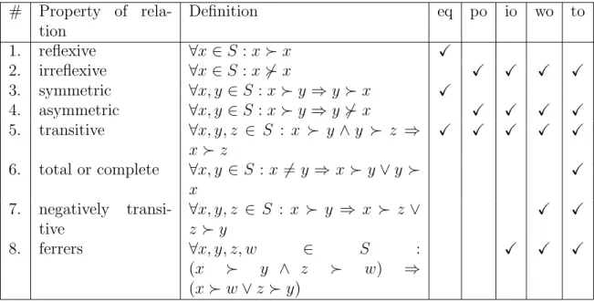
We recall some basic properties and definitions concerning binary relations used in this thesis (see [Fishburn, 1985] for a comprehensive treatment of the same). Let ≻ be a binary relation on a set S, i.e., ≻⊆ S×S. We say that ≻ is an equivalence (eq), a (strict) partial order (po), an interval order (io), a weak order (wo) or a total order (to), as defined in Table 2.1.
A total order is also a weak order; a weak order is also an interval order; and an interval order is also a strict partial order.
2.2
Qualitative Preferences
The problem we are interested in this research has to do with representing qualitative preferences over multiple attributes and reasoning with them to find the most preferred among a set of alternatives. Qualitative preferences over a setSare typically represented in the form of a binary relation ≻P⊆ S ×S such that for any two elements u, v ∈ S, u≻P v if and only if u is preferred to v.
# Property of rela-tion Definition eq po io wo to 1. reflexive ∀x∈S :x≻x X 2. irreflexive ∀x∈S :x6≻x X X X X 3. symmetric ∀x, y ∈S :x≻y⇒y≻x X 4. asymmetric ∀x, y ∈S :x≻y⇒y6≻x X X X X 5. transitive ∀x, y, z ∈ S : x ≻ y∧y ≻ z ⇒ x≻z X X X X X 6. total or complete ∀x, y ∈S : x6= y⇒ x≻ y∨y ≻ x X 7. negatively transi-tive ∀x, y, z ∈ S : x ≻ y ⇒ x ≻ z ∨ z ≻y X X 8. ferrers ∀x, y, z, w ∈ S : (x ≻ y ∧ z ≻ w) ⇒ (x≻w∨z ≻y) X X X
Table 2.1 Properties of binary relations
We focus only on strict partial order preference relations, i.e., relations that are
bothirreflexive and transitive, because transitivity is a natural property of any rational
preference relation [Morgenstern and Von Neumann, 1944, French, 1986a, Mas-Colell et al., 1995], and irreflexivity ensures that the preferences are strict.
With respect to any strict partial order preference relation ≻P, we say that two elements u and v are indifferent, denoted u ∼P v, whenever u 6≻P v and v 6≻P u. For preference relations ≻i,≻′i, and ≻d, we denote the corresponding indifference relation by∼i, ∼′i,∼ and ∼d respectively. We will drop the subscripts whenever they are understood from the context.
Proposition 1. For any strict partial order preference relation ≻P, the corresponding
indifference relation ∼P is reflexive and symmetric.
Proof. ∼P is reflexive becauseu6≻P uby the irreflexivity of≻P; it is symmetric because
u∼P v ⇔u6≻P v∧v 6≻P u⇔v ∼P u.
It is important to note that indifference with respect to a strict partial order is not necessarily transitive. For instance, ≻X= {(b, c)} is a strict partial order on the set
{a, b, c} with b∼X a, a∼X c but b ≻X c.
2.2.1 Qualitative Preference Languages
Let V ={Xi}be a set of preference variables, each with a domain Di. An outcome α ∈ O is a complete assignment to all the preference variables, denoted by the tuple α := hα(X1), α(X2), . . . , α(Xm)i such that α(Xi) ∈ Di for each Xi ∈ V. The set of all possible outcomes is given by O =QXi∈V Di.
Brafman’s seminal work [Brafman et al., 2006] attempts to address the problem of representing and reasoning with qualitative preferences by introducing preference
net-works that capture: (a) intra-variable or intra-attribute preferences specifying
prefer-ences over the domains of attributes; (b) therelative importance among the attributes. Therefore, we consider a preference language for specifying: (a) conditional intra-variable preferences≻i that are strict partial orders (i.e., irreflexive and transitive relations) over Di; and (b) conditional relative importance preferences that are strict partial orders over V.
Definition 1(Intra-variable Preference [Brafman et al., 2006]). Intra-variable preference
with respect to a attribute Xi (denoted ≻i), is an irreflexive, transitive and complete
binary preference relation on Di. ∀u, v ∈Di :u ≻i v iff u is preferred to v with respect
to Xi.
The intra-variable preference relation can be conditional in some settings, and in that case, the preferences over the values of a variable Xi may be influenced by the values assigned to a set of parent variables P a(Xi). The parent variables are said to “influence” the preference over the values of Xi, and the the the variable Xi is said to
be dependent on the variables in P a(Xi). Thus, there is a mapping from the set of all
possible assignments of the parent variables P a(Xi) to a set of intra-variable preference relations {≻i}.
A setX ⊆ X of attributes is said to bepreferentially independentof the setY =X \X of attributes if none of the variables in X are dependent on any of the variables in Y and vice versa. When the two sets contain exactly one variable each, then we simply say that the variables are preferentially independent of each other.
Definition 2 (Relative Importance [Brafman et al., 2006]). Relative importance
pref-erence with respect to the non-functional attributes X (denoted ), is an irreflexive,
transitive binary preference relation on X such that Xi Xj iff Xi is relatively more
important than Xj.
As with intra-variable preferences, relative importance may also be conditional. Con-ditional relative importance is specified as a preference relation on the set of variables conditioned on the values assigned to a set ofselector variables.
2.2.2 Representing Qualitative Preferences: CP-nets and TCP-nets
Preference networks [Boutilier et al., 2004, Brafman et al., 2006] offer a compact, directed graph representation of intra-variable and relative importance qualitative pref-erences. The nodes of the graph represent the attributes (X), with the node annotations representing the intra-variable preferences under various conditions specified in terms of the valuations of a set of other parent variables. There are various types of edges repre-senting the conditional intra-variable dependency (between a variable and its parents) and the relative importance preferences among the attributes.
CP-nets [Boutilier et al., 2004] specify conditional intra-variable preferences ≻i over a set of variables V. Each node in the graph corresponds to a variable Xi ∈ V, and
each dependency edge (Xi, Xj) in the graph captures the fact that the intra-variable
preference≻j with respect to variableXj is dependent (or conditioned) on the valuation of Xi. For any variable Xj, the set of variables {Xi : (Xi, Xj)is an edge} that influence ≻j are called the parent variables, denoted P a(Xj). Each node Xi in the graph is
associated with aconditional preference table (CPT) that maps all possible assignments to the parents P a(Xi) to a total order over Di. An acyclic CP-net is one that does not contain any dependency cycles.
TCP-nets [Brafman et al., 2006] extend CP-nets by allowing additional edges (Xi, Xj) to be specified, describing the relative importance among variables (Xi Xj). Each relative importance edge could be either unconditional (directed edge) or conditioned on a set of selector variables (analogous to parent variables in the case of intra-variable preferences). Each edge (Xi, Xj) describing conditional relative importance is undirected and is associated with a table (analogous to the CPT) mapping each assignment of the selector variables to either XiXj or vice versa. Figure 2.1 illustrates a TCP-net.
A
B
C
0≻A1 A= 0 : 0≻C1 A= 0 : 1≻B0 A= 1 : 0≻B1 A= 1 : 1≻C0Figure 2.1 Example of a TCP-net with 3 binary variables, namely A, B and C. It encodes the fact that the preference over values of B and C are dependent on the value assigned to the variable A, and that it is relatively more important to have a preferred valuation for the variableB in comparison to having a preferred valuation forC. The intra-attribute preferences are given in the boxes next to the variables.
An extended preference language due to Wilson [Wilson, 2004b, Wilson, 2004a] allows arbitrary preference statements of the form y : x ≻i x′[Z] where X ∈ X, x, x′ ∈ DX, y∈ Y ⊆ X \{X}, Z ⊆ X \Y\{X}.
2.2.3 Reasoning with Qualitative Preferences: Ceteris Paribus Semantics
Ceteris paribus is a Latin word that stands for “all else being equal”. A formal semantics in terms of theceteris paribus interpretation for preference languages involving conditional intra-variable and relative importance preferences (CP-nets and TCP-nets) was given by Brafman et al. in [Brafman et al., 2006].
A set X ⊆ X of attributes is preferentially independent of the set Y = X \X of attributes iff for all x1, x2 ∈QXi∈XDi; y1, y2 ∈QXi∈Y Di, we have: x1y1 is preferred to
x2y1 (denoted x1y1 ≻x2y1, where≻ is the preference relation on complete assignments to all attributes) iff x1y2 is preferred to x2y2 (i.e.,x1y2 ≻x2y2). We then say thatx1 is preferred to x2 ceteris paribus, i.e., “all else being equal”.
Given two preferentially independent attributes Xi and Xj, Xi is relatively more
important than Xj, denoted by XiXj, if
∀w∈QXl∈W Dl, where W =X − {Xi, Xj}
∀x1, x2 ∈Di,∀ya, yb ∈Dj :x1 ≻i x2 ⇒x1yaw≻x2ybw
Note thatx1yaw≻x2ybweven if yb ≻j ya, as any worsening of Xj is preferred to any worsening of Xi.
2.2.4 Dominance Testing
One of the important tasks in reasoning with qualitative intra-variable and relative importance preferences is dominance testing, i.e., given two complete assignments to variables or outcomes, determine whether one outcome is preferred to (dominates) the other. There are several ways in which one could define dominance between two out-comes. We list here two definitions based on the ceteris paribus semantics that require the existence of a sequence of outcomes called the flipping sequence. A flip from one outcome to the next in the sequence represents the change of one or more variables in
the outcome under certain conditions, while the outcomes are equal with respect to all other variables.
Definition 3 (Worsening flipping sequence: adapted from [Brafman et al., 2006]). A
sequence of outcomes α=γ1, γ2,· · ·γn−1, γn=β such that
α=γ1 ≻◦ γ2 ≻◦ · · · ≻◦ γn−1 ≻◦ γn=β
is a worsening flipping sequence with respect to a set of preference statements if
and only if, for 1≤i < n1, either
1. (V-flip) outcome γi is different from the outcome γi+1 in the value of exactly one
variable Xj, andγi(Xj)≻j γi+1(Xj), or
2. (I-flip) outcome γi is different from the outcome γi+1 in the value of exactly two
variables Xj and Xk, γi(Xj)≻j γi+1(Xj), andXj Xk.
The V-flips are induced directly by the conditional intra-variable preferences≻i, and the I-flips are additional flips induced by the relative importance over variables in conjunction with ≻i. Note that the notion of an I-flip in this definition revises the one presented in [Brafman et al., 2006] in order to accurately reflect the semantics of ≻◦ 2. Furthermore, this definition adapts the original definition such that flips are worsening rather than improving. Given a TCP-net N and a pair of outcomes α and β, Brafman et al. have shown that α ≻◦ β with respect to N if and only if there is a worsening flipping sequence with respect to N fromα to β.
An issue with dominance testing with respect to ≻◦ is that the interpretation of relative importance statements is pairwise, as illustrated by Wilson in [Wilson, 2004b, Wilson, 2004a]. In this case, I-flips allowonly two variables to be flipped at a time. On
1We assume the dominance relation is irreflexive and transitive in this thesis.
2Specifically, Definition 3 relaxes the stronger requirement (see Definition 13 in [Brafman et al., 2006])
that “γi+1(Xj)≻jγi(Xj) andγi(Xk)≻kγi+1(Xk)” to a weaker requirement that “γi+1(Xj)≻jγi(Xj)”
the other hand, Wilson’s extended semantics [Wilson, 2004b, Wilson, 2004a] (denoted
≻w) defines a worsening I-flip to allow multiple variables to be changed at a time in order to produce a worse outcome. This generalizes the search forflipping sequences to a search for swapping3 sequences.
Definition 4 (Worsening flipping sequence with revised I-flip: adapted from [Wilson, 2004b, Wilson, 2004a]). A sequence of outcomes α=γ1, γ2,· · ·γn−1, γn=β such that
α=γ1 ≻w γ2 ≻w · · · ≻w γn−1 ≻w γn=β
is a worsening flipping sequence with respect to a set of preference statements if
and only if, for 1≤i < n, either
1. (V-flip) as in Definition 3
2. (I-flip) outcome γi is different from the outcome γi+1 in the value of variables Xj
and Xk1, Xk2,· · ·Xkn, γi(Xj)≻j γi+1(Xj), and XjXk1, XjXk2,· · · , XjXkn. Given a TCP-net N and a pair of outcomesαandβ, according to Wilson’s semantics we say that N entails α ≻w β iff there is a worsening flipping sequence with respect to
N fromα to β.
Dominance testing has been shown to be PSPACE-complete [Goldsmith et al., 2008] for CP-nets and TCP-nets under all the above semantics which are based on the ceteris paribus interpretation of qualitative preferences.
2.3
Compositional Systems
A compositional system consists of a repository of pre-existing components from which we are interested in assembling compositions that satisfy a pre-specified function-ality. Formally, a compositional system is a tuplehR,⊕,|=i where:
3To simplify the terminology, we will henceforth use the termflipping sequence to refer to Wilson’s
• R={W1, W2. . . Wr} is a set of available components,
• ⊕ denotes a composition operator that functionally aggregates components and encodes all the functional details of the composition. ⊕ is a binary operation on components Wi, Wj in the repository that produces a composition Wi⊕Wj. • |= is a satisfaction relation that evaluates to true when a composition satisfies
some pre-specified functional properties.
Definition 5 (Compositions, Feasible Compositions and Extensions). Given a
compo-sitional systemhR,⊕,|=i, and a functionality ϕ, a compositionC =Wi1⊕Wi2⊕. . . Win
is an arbitrary collection of components Wi1, Wi2, . . . , Win s.t. ∀j ∈[1, n] :Wij ∈R.
i. C is a feasible composition whenever C |=ϕ;
ii. C is a partial feasible compositionwhenever∃Wi1. . . Win ∈R :C⊕Wi1⊕. . .⊕Win is a feasible composition; and
iii. C⊕Wi is a feasible extension of a partial feasible compositionC whenever C⊕Wi is a feasible or a partial feasible composition.
2.3.1 Functional Composition
Given a compositional system hR,⊕,|=i and a functionality ϕ, an algorithm that produces a set of feasible compositions (satisfying ϕ) is called a functional composition
algorithm. The most general class of functional composition algorithms we consider can
be treated asblack boxes, simply returning a set of feasible compositions satisfying ϕ in a single step. Some other functional composition algorithms proceed by computing the set of feasible extensions of partial feasible compositions incrementally.
Definition 6 (Incremental Functional Composition Algorithm). A functional
C and the desired functionality ϕ, the algorithm computes the set of feasible extensions
to C.
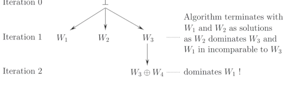
An incremental functional composition algorithm can be used to compute the feasible compositions by recursively invoking the algorithm on the partial feasible compositions it produces starting with the empty composition (⊥), and culminating with a set of feasible compositions satisfying ϕ. In this sense, incremental functional composition algorithms are similar to their “black box” counterparts. However, (as we later show in Chapter 4.2.5) in contrast to their “black box” counterparts, incremental functional composition algorithms can be exploited in the search for the most preferred feasible compositions, by interleaving each step of the functional composition algorithm with the optimization of the valuations of non-functional attributes (with respect to the user preferences). This allows us to develop algorithms that can eliminate partial feasible compositions that will lead to less preferred feasible compositions from further consid-eration early in the search.
Different approaches to functional composition, (e.g., [Traverso and Pistore, 2004, Lago et al., 2002, Baier et al., 2008, Passerone et al., 2002]) differ in terms of (a) the languages used to represent the desired functionality ϕ and the compositions, and (b) the algorithms used to verify whether a composition C satisfiesϕ, i.e.,C |=ϕ. We have intentionally abstracted the details of how functionalityϕis represented (e.g., transition systems, logic formulas, plans, etc.) and how a composition is tested for satisfiability (|=) against ϕ, as the primary focus of our work is orthogonal to details of the specific methods used for functional composition.
2.3.2 Preferences over Non-functional Attributes
We now turn to the non-functional aspects of compositional systems. In addition to obtaining functionally feasible compositions, users are often concerned about the
non-functional aspects of the compositions, e.g., the reliability of a composite Web service. In such cases, users seek themost preferred compositions among those that are functionally feasible, with respect to a set of non-functional attributes describing the components. In order to compute the most preferred compositions, it is necessary for the user to specify his/her preferences over a set of non-functional attributes X.
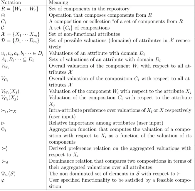
Notation. In general, for any relation≻P, we use the same to denote the transitive closure of the relation as well, and 6≻P or ¬ ≻P to denote its complement. The list of notations used in this thesis are given in Table 2.2.
Representing Multi-Attribute Preferences. Following the representation scheme introduced by Boutilier et al. [Boutilier et al., 2004] and Brafman et al. [Brafman et al., 2006], we model the user’s preferences with respect to multiple attributes in two forms: (a) intra-attribute preferences with respect to each non-functional attribute in
X, and (b) relative importance over all attributes.
Definition 7 (Intra-attribute Preference). The intra-attribute preference relation,
de-noted by ≻i is a strict partial order (irreflexive and transitive) over the possible
valua-tions of an attribute Xi ∈ X. ∀u, v ∈ Di : u ≻i v iff u is preferred to v with respect to
Xi.
Definition 8 (Relative Importance). The relative importance preference relation,
de-noted byis a strict partial order(irreflexive and transitive) over the set of all attributes
X. ∀Xi, Xj ∈ X :XiXj iff Xi is relatively more important than Xj.
Notation Meaning
R={W1· · ·Wr} Set of components in the repository
⊕ Operation that composes components fromR
Ci A composition or collection4of a set of components from R
C A set {Ci}of compositions
X ={X1· · ·Xm} Set of non-functional attributes
D={D1· · ·Dm} Set of possible valuations (domains) of attributes in X respec-tively
ui, vi, ai, bi· · · ∈Di Valuations of an attribute with domainDi
Ai, Bi· · · ⊆Di Sets of valuations of an attribute with domainDi
VWi Overall valuation of the component Wi with respect to all at-tributes X
VCi Overall valuation of the composition Ci with respect to all at-tributes X
VWi(Xj) Valuation of the componentWi with respect to the attributeXj VCi(Xj) Valuation of the composition Ci with respect to the attribute
Xj
≻i,≻X Intra-attribute preference over valuations ofXiorXrespectively (user input)
Relative importance among attributes (user input)
Φi Aggregation function that computes the valuation of a
compo-sition with respect to Xi as a function of the valuation of its components
≻′
i Derived preference relation on the aggregated valuations with respect toXi
≻d Dominance relation that compares two compositions in terms of their aggregated valuations over all attributes
Ψ≻(S) The non-dominated set of elements inS with respect to ≻ ϕ User specified functionality to be satisfied by a feasible
compo-sition
CHAPTER 3.
Efficient Preference Reasoning Techniques
As we have seen in Chapter 1, CP-nets [Boutilier et al., 2004], TCP-nets [Brafman et al., 2006] and their extensions [Wilson, 2004b, Wilson, 2004a] capture qualitative intra-variable preferences and relative importance over a set of variables. Dominance testing for these languages has been shown to be PSPACE-complete [Goldsmith et al., 2008] based on the ceteris paribus (“all else being equal”) interpretation of preferences.
3.1
Efficient Dominance Testing for Unconditional
Preferences
In this section, we attempt to alleviate the complexity of dominance testing in TCP-nets by restricting the preference language to unconditional qualitative preferences. We consider TUP-nets, an unconditional fragment of TCP-nets. We introduce a dominance relation for TUP-nets and compare it with its unconditional counterparts for TCP-nets and their variants. We provide a polynomial time algorithm for dominance testing for TUP-nets. TUP-nets are not special cases of already known restrictions of CP-/TCP-nets for which polynomial time dominance testing algorithms exist [Boutilier et al., 2004].
3.1.1 A Language for Unconditional Preferences
LetX ={Xi}be a set of variables, each with a domain Di. An outcome αis a com-plete assignment to all the variables, denoted by the tupleα:=hα(X1), α(X2), . . . , α(Xm)i
such that α(Xi) ∈ Di for each Xi ∈ X. We consider a preference language LT U P for specifying: (a) unconditional intra-variable preferences ≻i that are strict partial orders (i.e., irreflexive and transitive relations) overDi for each Xi ∈ X; and (b) unconditional relative importance preferences that are strict partial orders over X.
Let LCP, LT CP andLExt denote the preference languages of CP-nets, TCP-nets (an extension of CP-nets) and Wilson’s extension to TCP-nets respectively. We note that:
• LT U P allows the expression of relative importance while LCP does not; and LCP allows the expression of conditional intra-variable preferences whileLT U P does not. • LT U P is less expressive than LT CP because it does not allow the expression of
conditional preferences.
• When restricted to unconditional preferences, LT CP =LT U P.
• LExt is more expressive than LT CP [Wilson, 2004b, Wilson, 2004a], and hence, LT U P as well.
3.1.2 Dominance Testing for LT U P
We now provide a polynomial time dominance testing approach for LT U P. We pro-ceed by defining a relation i (for each variable Xi ∈ X) that is derived from≻i. Definition 9 (i). ∀u, v ∈Di :u i v ⇔u=v∨u≻i v
Since ≻i is a strict partial order (irreflexive and transitive), it can be shown that i is a preorder (reflexive and transitive). We next define dominance of α over β with respect to {≻i}and using a first order logic formula.
Definition 10 (Dominance for Unconditional Preferences). Given input preferences
{≻i} and , and a pair of outcomes α and β, we say that α dominates β (denoted
∃Xi :α(Xi)≻i β(Xi)
∧ ∀Xk : (XkXi∨Xk ∼Xi)⇒ α(Xk) k β(Xk)
where Xk ∼Xi ⇔Xk 6Xi∧Xi 6Xk, and Xi is called the witness of the relation.
Intuitively, this definition of dominance of α over β (i.e., α ≻• β) requires that α
is preferred to β with respect to at least one variable, namely the witness. Further,
it requires that for all variables that are relatively more important than or indifferent to the witness, α is either equal to or is preferred to β. In Example 12, α ≻• β, with witness X1.
3.1.2.1 Properties of Dominance
We now proceed to analyze some properties of ≻•. Specifically, we would like to ensure that ≻• has two desirable properties of preference relations: irreflexivity and transitivity, which make it a strict partial order. First, it is easy to see that ≻• is irreflexive, due to the irreflexivity of ≻i (since it is a partial order).
Proposition 2 (Irreflexivity of ≻•). ∀α:α6≻• α.
The above proposition ensures that the dominance relation ≻• is strict over compo-sitions. In other words, no composition is preferred over itself. Regarding transitivity, we observe that ≻• is not transitive when ≻
i and are both arbitrary strict partial orders, as illustrated by the following example.
Example 1. Let X = {X1, X2, X3, X4}, and for each Xi ∈ X : Di = {ai, bi} with ai ≻i bi. Suppose that X1X3 and X2X4. Let α=ha1, a2, b3, b4i, β =hb1, a2, a3, b4i
and γ =hb1, b2, a3, a4i. Clearly, we have α ≻• β (with X1 as witness), β ≻• γ (with X2
as witness), but there is no witness for α≻• γ, i.e., α6≻• γ according to Definition 10.
Because transitivity of preference is a necessary condition for rational choice [Morgen-stern and Von Neumann, 1944, French, 1986a], we proceed to investigate the possibility
Xk Xi Xi Xj Xj Xk Xi Xj Xk Xk∼⊲Xi (a) (b) (c) Xk⊲Xi Figure 3.1 XiXj ∧(XkXi∨Xk ∼Xi)
of obtaining such a dominance relation by restricting. In particular, we find that≻• is transitive whenis restricted to a special family of strict partial orders, namelyinterval
orders as defined below. We prove that such a restriction is necessary and sufficient for
the transitivity of≻•.
Definition 11 (Interval Order). A binary relationR ⊆ X × X is an interval order iff it
is irreflexive and satisfies the ferrers axiom [Fishburn, 1985]: for all Xi, Xj, Xk, Xl ∈ X,
we have:
(XiRXj ∧XkRXl)⇒(XiRXl∨XkRXj)
We now proceed to establish the transitivity of ≻• when is an interval order. We make use of two intermediate propositions 3 and 4 that are needed for the task.
In Proposition 3, we prove that if an attribute Xi is relatively more important than Xj, then Xi is not more important than a third attribute Xk implies that Xj is also not more important than Xk. This will help us prove the transitivity of the dominance relation. Figure 3.1 illustrates the cases that arise.
Proposition 3. ∀Xi, Xj, Xk :XiXj ⇒
(XkXi∨Xk ∼ Xi)⇒(XkXj ∨Xk ∼Xj)
The proof follows from the fact that is a partial order. Proof.
Xi Xj′ Xj Xi X′ i Xj (a) (b) (c) Xi Xj Xi X′ j Xj Xi Xi′ Xj (d) (e) X′ j Xj Xi Xi′ (f) Xu=Xj Xu=Xi Xv=Xi Xv=Xj Contradiction! (⊲is aninterval order) Figure 3.2 Xi ∼ Xj 1. XiXj (Hyp.) 2. XkXi∨Xk ∼ Xi (Hyp.) Show XkXj ∨Xk ∼Xj
(a) XkXi ⇒XkXj By transitivity of and (1.); see Figure 3.1(a) (b) Xk ∼Xi ⇒XkXj∨Xk∼ Xj
i. Xk ∼ Xi (Hyp.)
ii. (XkXj)∨(XjXk)∨ (Xk ∼ Xj) Always; see Figure 3.1(b,c) iii. Xj Xk ⇒XiXk (1.) Contradiction!
iv. XkXj ∨Xk ∼Xj (2.2.ii., iii.)
3. XiXj ⇒
(XkXi∨Xk ∼ Xi)⇒(XkXj ∨Xk ∼ Xj)
(1.,2.1,2.2) Proposition 4 states that if attributes Xi, Xj are such that Xi ∼ Xj then at least
one of them,Xu is such that with respect to the other,Xv, there is no attributeXkthat is less important while at the same time Xk ∼ Xu. This result is needed to establish the transitivity of the dominance relation.
Proposition 4. If is an interval order, then ∀Xi, Xj, u6=v, Xi ∼Xj
⇒ ∃Xu, Xv ∈ {Xi, Xj},∄Xk : (Xu ∼ Xk∧XvXk).
Proof. Let Xi ∼ Xj, and Xi′ and Xj′ be variables that are less important than Xi
and Xj respectively (if any). Figure 3.2 illustrates all the possible cases that arise. Figure 3.2(a, b, c, d, e) illustrates the cases whenat most one of X′
i and Xj′ exists, and in each case the claim holds trivially. For example, in the cases of Figure 3.2(a, b, c), bothXu =Xi;Xv =Xj and Xu =Xj;Xv =Xi satisfy the implication, and in the cases of Figure 3.2(d, e), the corresponding satisfactory assignments to Xu and Xv are shown in the figure. The final case (Figure 3.2(f)) corresponds tonot being an interval order (see Definition 11). Hence, the proposition holds in all cases.
The above proposition reflects the interval order property of the relation, and relates to Example 1 in which ≻• was shown to be intransitive whenis not an interval order. In fact, if relative importance was defined as a strict partial order instead, it is easy to see that the above proof does not hold. Given that α≻• β with witness X
i and β ≻• γ with witness X
j, the above proposition guarantees that one among Xi and Xj can be chosen as a potential witness for α ≻• γ so that the conditions demonstrated in Example 1 are avoided. Using the propositions 3 and 4, we are now in a position to prove the transitivity of ≻• in Proposition 5.
Proposition 5 (Transitivity of≻•). ∀α, β, γ,
α≻• β∧β ≻• γ ⇒α≻• γ when is an interval order.
The proof proceeds by considering all possible relationships between Xi, Xj, the respective attributes that are witnesses of the dominance of α over β and β over γ. Lines 5,6,7 in the proof establish the dominance of α over γ in the cases Xi Xj, XjXi andXi ∼Xj respectively. In the first two cases, the more important attribute amongXi and Xj is shown to be the witness for α≻• γ with the help of Proposition 3; and in the last case we make use of Proposition 4 to show that at least one ofXi, Xj is a witness for α≻• γ.
Proof.
1. α≻• β (Hyp.) 2. β ≻• γ (Hyp.)
3. ∃Xi : α(Xi)≻′iβ(Xi) (1.) 4. ∃Xj : β(Xj)≻′jγ(Xj) (2.)
Three cases arise: XiXj(5.),XjXi(6.) andXi ∼ Xj(7.). 5. XiXj ⇒α ≻• γ 1. XiXj (Hyp.) 2. β(Xi)′iγ(Xi) (2.,5.1.) 3. α(Xi)≻′iγ(Xi) (3.,5.2.) 4. ∀Xk : (XkXi∨Xk∼ Xi)⇒α(Xk)′kγ(Xk) i. Let XkXi∨Xk ∼Xi (Hyp.) ii. α(Xk)′kβ(Xk) (1.,5.4.i.)
iii. XkXj ∨Xk ∼Xj (5.4.i., P roposition 3)
iv. β(Xk)′kγ(Xk) (2.,5.4.iii.) v. α(Xk)′kγ(Xk) (5.4.ii.,5.4.iv.) 5. XiXj ⇒α≻• γ (5.1.,5.3.,5.4.) 6. XjXi ⇒α ≻• γ
1. This is true by symmetry of Xi, Xj in the proof of (5.); in this case, it can easily be shown that α(Xj)≻′iγ(Xj) and ∀Xk : (Xk Xj ∨Xk ∼ Xj) ⇒ α(Xk)′kγ(Xk).
7. Xi ∼ Xj ⇒α≻• γ 1. Xi ∼ Xj (Hyp.)
2. ∃Xu, Xv ∈ {Xi, Xj}:Xu 6=Xv ∧∄Xk : (Xu ∼Xk∧Xv Xk) (7.1., P roposition 4)
3. Without loss of generality, suppose that Xu =Xi, Xv =Xj (Hyp.). 4. β(Xi)′iγ(Xi) (2.,7.1.)
5. α(Xi)≻′iγ(Xi) (3.,7.4.)
6. ∀Xk :XkXi ⇒α(Xk)′kγ(Xk). i. XkXi (Hyp.)
ii. α(Xk)′kβ(Xk) (1.,7.6.i.)
iii. XkXj ∨Xk ∼Xj Because XjXk Contradicts (7.1.,7.6.i.)!
iv. β(Xk)′kγ(Xk) (2.,7.6.iii.) v. α(Xk)′kγ(Xk) (7.6.ii.,7.6.iv.) 7. ∀Xk :Xk ∼Xi ⇒α(Xk)′kγ(Xk)
i. Xk ∼ Xi (Hyp.)
ii. α(Xk)′kβ(Xk) (1.,7.7.i.)
iii. XkXj ∨Xk ∼Xj Because XjXk Contradicts (7.2.,7.3.)!
iv. β(Xk)′kγ(Xk) (2.,7.7.iii.) v. α(Xk)′kγ(Xk) (7.7.ii.,7.7.iv.) 8. ∀Xk :XkXi∨Xk∼ Xi ⇒α(Xk)′kγ(Xk) (7.6.,7.7.) 9. Xi ∼ Xj ⇒α≻• γ (7.5.,7.8.) 8. (XiXj∨Xj Xi∨Xi ∼Xj)⇒α≻• γ (5.,6.,7.) 9. α≻• β∧β ≻• γ ⇒α≻• γ (1.,2.,8.)
From Propositions 2 and 5, we have the first main result of this chapter as follows.
Theorem 1. ≻• is a strict partial order when intra-attribute preferences≻
i are arbitrary
X′ j Xj Xi X′ i
Figure 3.3 A 2⊕2 substructure, not an Interval Order
The above theorem applies to all partially ordered intra-variable preferences and a wide range of relative importance preferences including total orders, weak orders and semi orders [Fishburn, 1985] which are all interval orders. Having seen in Example 1 that the transitivity of ≻• does not necessarily hold when is an arbitrary partial order, a natural question that arises here is whether there is a condition weaker than the interval order restriction on that still makes ≻• transitive. The answer turns out to be negative, which we show next. We make use of a characterization of interval orders by Fishburn in [Fishburn, 1985], which states that is an interval order if and only if 2⊕2*, where 2⊕2 is a relational structure shown in Figure 3.3. In other words, is an interval order if and only if it has no restriction of itself that is isomorphic to the partial order structure shown in Figure 3.3.
Theorem 2. For arbitrary partially ordered intra-attribute preferences ≻• is transitive
only if relative importance is an interval order.
Proof. Assume that is not an interval order. This is true if and only if 2⊕2 ⊆ .
However, we showed in Example 1 that in such a case≻• is not transitive. Hence,≻• is transitive only if relative importance is an interval order.
For the special case of = ∅, i.e., when there are no relative importance prefer-ences specified, (Xk ∼ Xi) always holds for any pair of variables Xi, Xk ∈ X. Hence, dominance testing reduces to:
α≻• β ⇔ ∃X
i :α(Xi)≻i β(Xi)∧ ∀Xk :α(Xk) k β(Xk)
3.1.2.2 Complexity of Dominance Testing
We now analyze the complexity of evaluating α ≻• β in terms of the following parameters: (a) number of variables m = |X |; (b) size of the domains of variables n=maxXi∈X|Di|; (c) size of the intra-variable preferencekint=maxXi∈X| ≻i |; and (d) size of the relative importance preference relation krel =||.
The evaluation of ≻• (Definition 10) involves the evaluation of two clauses for each variableXi ∈ X. The first clause checks ifα(Xi)≻i β(Xi). The complexity of evaluating the first clause for each Xi is thus O(kint). For each Xi, the second clause checks if the implication holds for each Xk ∈ X − {Xi}. The left hand side of the implication computesXkXi∨Xk ∼Xi, or equivalentlyXi 6Xkand has complexityO(krel); and the right hand side computes α(Xk) k β(Xk) and has complexity O(kint) (similar to the complexity of the first clause). Hence, the overall complexity of evaluating α ≻• β is O m kint+m(krel +kint)
, or O m2(k
int+krel)
. Since krel = | | (and hence bounded by m2); and k
int =| ≻i | (and hence bounded by n2), the complexity can also be expressed as O m2(m4+n4)in terms of the number of variables and domain size of variables.
3.1.3 Semantics: Relationship Between ≻◦, ≻w & ≻•
We investigate the relationship between the semantics ≻◦, ≻•, and ≻w for the lan-guage LT U P. We show that:
a) ≻•⊆≻w
b) ≻•=≻w when is an interval order
c) (≻•)⋆ =≻w, where (≻•)⋆ is the transitive closure of≻•
Theorem 3. ≻• ⊆ ≻w. Proof.
We will show that α ≻• β⇒α ≻w β for any pair of outcomes α, β. Suppose that α ≻• β with witness X
i (see Definition 10). Define the sets L = {Xl : XiXl}, M ={Xl : (XlXi∨Xl ∼Xi)∧α(Xl)≻l β(Xl)∧Xl 6=Xi}, and
M′ ={X
l : (XlXi∨Xl ∼ Xi)∧α(Xl) =β(Xl)∧Xl=6 Xi}. Clearly, the sets{Xi}, L, M, M′ form a partition of X. Let X
t1, Xt2, . . . Xtn be an enumeration of M.
We now construct a sequence of outcomes γt1, γt2, . . . , γtn corresponding to variables Xt1, Xt2, . . . Xtn as follows. γt1 = hγt1(X1), γt1(X2), . . . γt1(Xm)i such that γt1(Xt1) =
α(Xt1) and ∀Xj ∈ X − {Xt1} : γt1(Xj) = β(Xj). Similarly, construct the ith outcome γti = hγti(X1), γti(X2), . . . γti(Xm)i such that γti(Xti) = α(Xti); and ∀Xj ∈ X − {Xti} : γti(Xj) =γti−1(Xj).
Now, we make use of Definition 4 to compare these outcomes with respect to ≻w. γt1 ≻w βbecauseγt1(Xt1) =α(Xt1)≻t1 β(Xt1) withγt1andβ being equal in all variables other than Xt1 (V-flip). Also γti+1 ≻w γti because γti+1(Xti) = α(Xti) ≻ti γti(Xti) = β(Xti), with γti+1 and γti being equal in variables other than Xti. For the last outcome in this sequence γt1, . . . , γtn, we have α ≻w γtn b