ADAPTING TO UNKNOWN DISTURBANCE
AUTOCORRELATION IN REGRESSION WITH LONG MEMORY
* byJavier Hidalgo and Peter M Robinson
London School of Economics and Political Science
Contents: Abstract 1. Introduction
2. Adaptive Estimation of β
3. Monte Carlo Study of the Finite-Sample Behaviour 4. Proof of Theorem 2.1 Appendix A Appendix B References Tables 1 – 4
The Suntory Centre
Suntory and Toyota International Centres for
Economics and Related Disciplines
London School of Economics and Political Science Discussion Paper Houghton Street
No. EM/01/427 London WC2A 2AE September 2001 Tel.: 020 – 7955 6698
*
The first author’s research was supported by ESRC Grant R000238212. The second author’s research was supported by ESRC Grant R000235892 and R000238212 and a Leverhulme Trust Personal Research Professorship. Stepana Lazarova carried out the Monte Carlo work, modifying a computer program written by Josu Arteche, who carried out the Monte Carlo in the original version of this paper. The paper has been improved in response to comments of three referees and a co-editor.
Abstract
We show that it is possible to adapt to nonparametric disturbance auto-correlation in time series regression in the presence of long memory in both regressors and disturbances by using a smoothed nonparametric spectrum estimate in frequency-domain generalized least squares. When the collective memory in regressors and disturbances is sufficiently strong, ordinary least squares is not only asymptotically inefficient but asymptotically non-normal and has a slow rate of convergence, whereas generalized least squares is asymptotically normal and Gauss-Markov efficient with standard convergence rate. Despite the anomalous behaviour of nonparametric spectrum estimates near a spectral pole, we are able to justify a standard construction of frequency-domain generalized least squares, earlier considered in case of short memory disturbances. A small Monte Carlo study of finite sample performance is included.
Keywords: Time series regression; long memory; adaptive estimation. JEL No.: C22
©
by the authors. All rights reserved. Short sections of text, not to exceed two paragraphs, may be quoted without special permission provided that full credit, including © notice, is given to the source.Contact address: Dr Javier Hidalgo, Department of Economics, London School of Economics and Political Science, Houghton Street, London WC2A 2AE. Email: [email protected]/
1. INTRODUCTION
Adaptive estimation in semiparametric models entails an estimate of the paramet-ric component achieving the same first-order efficiency when the nonparametric nuisance function is consistently estimated as when this function is known. It seems that such adaptive estimation was first established by Hannan (1963), in the context of linear time series regression with disturbance having nonparametric autocorrelation, the Gauss-Markov bound being attained. Hannan considered an approximate frequency-domain generalized least squares (GLS) estimate, using a smoothed nonparametric estimate of the disturbance spectral density. Even though the spectral estimate converges slowly, Hannan showed that nevertheless hisGLS estimate can have the same first order limit distribution as if the spec-tral density were completely known, or a known parametric function. The same idea was extended to more general semiparametric time series models, especially ones useful in econometrics, by Hannan(1965), Hannan and Terrell(1972,1973), Robinson (1976) and more recently by Robinson (1991), who also allowed for a data dependent smoothing in the spectral estimation and considered optimal choice of the smoothing number, and Phillips(1991) who considered this type of estimate in the presence of unit root regressors.
The regularity conditions required by Hannan (1963) and the subsequent au-thors are in many respects quite mild, in particular the disturbance spectral den-sity need only be bounded and bounded away from zero and satisfy mild smooth-ness conditions, so that stationary and invertible autoregressive moving averages are easily covered. However, there is now increasing awareness of the possibility of long memory in disturbances, which contradicts such specifications. The concept of long memory can be loosely defined in terms of theI(d)processes. We say that a covariance stationary, invertible process is I(d) if it has spectral density that behaves like Cλ−2d as frequency λ → 0+, for 0< C < ∞ and −1/2< d < 1/2. Then there is said to be negative memory if−1/2< d <0, short memory ifd= 0, and long memory if0< d <1/2. For d >1/2, a process can be said to be (non-stationary)I(d)if its kth integer difference is I(d−k), for−1/2< d−k <1/2, to cover unit root (I(1)) processes, for example. We can also define long memory relative to a spectral pole at some non-zero frequency, and will return to this possibility subsequently. In the context of the linear regression model
yt=α+β0xt+ut, t = 1,2, ..., (1.1)
where the scalar α and the p×1 vector β are unknown and the prime denotes transposition, long memory in the disturbanceut can occur if thep×1regressor
vectorxt does not wholly account for long memory in the dependent variable yt.
which can bridge the gap between short memory and unit root processes (which have recently played a considerable role in econometric modelling), especially as the latter occupy only one point in d-space, whereas stationary long memory processes take up an interval.
Initial study of the implications of long memory ut in (1.1) focussed on
or-dinary least squares (OLS) estimates of β. In case of deterministic, such as polynomial-in-t regressors, Yajima (1988,1991) found that OLS estimates can still be asymptotically normal, even if ut is non-Gaussian but a linear process.
However their asymptotic variance, indeed their rate of convergence, is adversely affected by the long memory in ut. Moreover, while the OLS estimates may not
necessarily have poor efficiency, they cannot achieve the Gauss-Markov bound, even for polynomial-in-t regressors, unlike in the case of short memory ut
consid-ered by Grenander(1954). In econometric applications, it is often reasonable to regard xt, or at least some elements of it, as stochastic. Here, even if xt and ut
are independent stationary processes, indeed possibly Gaussian ones, sufficiently strong collective memory leads to OLS having a slow rate of convergence and non-standard limiting distribution, specifically, as found by Robinson (1994a), if ut is I(d)and xt is I(dx) andd+dx >1/2. This outcome is consistent with the
familiar one in econometrics in which d = 0 and dx = 1, but the implications
are rather more serious because not only, as there, is the limit distribution less convenient for use in inference than the normal, but it depends ondanddx, which
are typically regarded as unknown when fractional models are entertained. Note also that not only is the conventional econometric approach to inference, based on OLS and an autocorrelation-consistent variance estimate (employing a smoothed nonparametric estimate of the spectral density of xtut, see e.g. Andrews, 1991)
inefficient (as usual) due to its dependence on an inefficient point estimate, but it is not even available due to the asymptotic non-normality.
To resolve this difficulty, Robinson and Hidalgo (1997) considered a class of frequency-domain weighted least squares (W LS) estimates. Based on observa-tions (x0
t, yt), t= 1, ..., n, define the discrete Fourier transforms ofxt andyt
wx(λ) = 1 (2πn)1/2 n X t=1 xteitλ, wy(λ) = 1 (2πn)1/2 n X t=1 yteitλ,
and the periodogram matrix and vector
Ixx(λ) =wx(λ)w∗x(λ), Ixy(λ) =wx(λ)wy∗(λ),
where ”∗” indicates transposition combined with complex conjugation. Now write b βφ= Ãn−1 X j=1 Ixx(λj)φ(λj) !−1Ãn−1 X j=1 Ixy(λj)φ(λj) ! , (1.2)
where φ(λ) is real-valued, even and periodic of period 2π and λj = 2πj/n, for
integerj. This is one of the W LS estimates considered by Robinson and Hidalgo (1997) (the other replacing sums by integrals and having the same first-order asymptotic properties, but being less convenient computationally). Omission of the frequency j = 0 (and j = n) entails sample-mean correction, and when φ(λ)≡1, bβφreduces to theOLS estimate ofβ for the model(1.1). Assume that ut has absolutely continuous spectral distribution function, so it has a spectral
densityf(λ)satisfying
γj =Cov(u1, u1+j) =
Z π
−π
f(λ) cos (jλ)dλ, j = 0,±1, ....
If, for allλ, f(λ)>0 andf(λ)is known then bβf−1 is an approximate GLS
esti-mate, achieving the Gauss-Markov bound under suitable conditions, in particular n1/2³βbf−1 −β
´ d
→ N¡0,Ω−1¢, (1.3) whereΩ= (2π)−1R−ππf−1(λ)dF(λ)and the matrix F (λ)satisfies
Γ(j) =E¡(x1−Ex1) (x1+j−Ex1)0 ¢ = Z π −π eijλdF(λ)
such that F (λ) has Hermitian nonnegative definite increments and is uniquely defined by the requirement that it is continuous from the right.
The result (1.3) was established by Robinson and Hidalgo(1997) under regu-larity conditions which permit arbitrarily strong stationary long memory in both xt and ut. Intuitively, whereas OLS has an asymptotic variance involving the
integral R−ππf(λ)dF(λ), which will not converge if the spectral mass of xt and
ut near zero frequency is collectively sufficiently great, this is no obstacle to
con-vergence of Ω because long memory in ut entails a zero, not a pole, in f−1(λ).
Thus, not only doesGLS have its usual desirable asymptotic Gauss-Markov effi -ciency properties, but it is also motivated in the present circumstances by being asymptotically normal, even whenOLS is not and has slow rate of convergence. Moreover, even whenOLS isn1/2
−consistent, it is easy to construct examples in whichOLS has very poor efficiency relative to GLS. Dahlhaus (1995) has also considered GLS under long memory ut, but for deterministic xt where, as noted
previously, OLS is typically asymptotically normal however strong the memory ofut, so thatGLS appears tofill a lesser gap than in the stochastic case.
As presented, (1.3) assumes f(λ) is known, which is unrealistic in applica-tions. Robinson and Hidalgo(1997)showed that(1.3)still goes through iff(λ)is a known function ofλ andfinitely many unknown parameters, and the latter are
replaced by n1/2-consistent estimates. However, correct parametric specification
off(λ) is here essential. For example ifut is specified as a fractional
autoregres-sive integrated moving average(F ARIM A)process but either the autoregressive or the moving average order is under-stated, or both are over-stated, then the estimate ofβ will not be asymptotically efficient and (1.3)will not hold. Indeed, the estimate may not then even be n1/2
−consistent and asymptotically normal, because the misspecification of autoregressive and/or moving average orders leads to an inconsistent spectral estimate, which in particular may be biased downwards such that the reciprocal of the estimatedf(λ)does not sufficiently compensate for the long memory in the manner discussed above. In view of the earlier discussion we would therefore like to adapt to nonparametricf(λ). This is accomplished in the present paper; we establish (1.3) after replacing f by a smoothed nonpara-metric estimate. We have found this to be a very difficult task, far more than whenut has short memory, especially in the context of the standard specification
of semiparametricGLS (one originally proposed for short memory ut) which we
use, that does not resort to special devices such as trimming near frequency zero in order to deal with the unpleasant properties of spectral estimates near a spec-tral pole. Indeed, even for known f, the result (1.3) was found by Robinson and Hidalgo(1997) to be considerably more difficult to establish under long memory than short memory, and some of our regularity conditions are no stronger than ones in that paper.
As in Robinson and Hidalgo(1997), we assumext is stationary. Nonstationary
xt can be considered, indeed Phillips(1991)analyzed a semiparametric GLS
esti-mate withI(1)xt (but short memoryut)but hisfindings were that GLSloses its
classical properties (c.f. (1.3)) then, indeed that a narrow-band estimate (about zero frequency) does as well, so that the unequal weighting entailed in GLS is redundant. This is due to the dominance of low frequencies inI(1)processes, and so a similar outcome might be expected in case of other nonstationary processes, especially in view of results of Robinson and Marinucci (1998). This type of outcome is not very interesting from the point of view of adaptive estimation, especially if (as in thext∼I(1)/ utvI(0)case) the limit distribution ofGLS is
not even normal. Now from our discussion of the convergence ofΩ, it appears that even for some nonstationaryxt, specificallyI(dx)ones for1/2≤dx <1, the zero
in f−1(λ) might ’compensate’, so as to lead to an outcome like (1.3). However
this would clearly require sufficiently strong long memory in ut relative to that
in xt ( d > dx−1/2 if ut v I(d)), even in case of known f no limit results are
yet available, and a modified construction would be needed such as one involving tapering, in view of other literature on nonstationary fractional processes. In the circumstances it seems desirable to deal with the stationary case first, stressing again that our inclusion of I(dx) processes for dx < 1/2 is considerably broader
than the class of I(0) processes sometimes erroneously referred to in the litera-ture as synonymous with stationarity, while our conditions are in other respects mostly undeniably mild. The stationarity assumption may itself be reasonable in the context of some financial data, while in any case it can sometimes be hard to distinguish a record of a nonstationary process from that of a stationary frac-tional one, for example compare realizations of a unit root process with ones of a F ARIM A(1,0.45,0) with autoregressive parameter0.95.
Our assumptions requiref to have a pole, if at all, at frequency zero only, but because we use a standard construction of aGLS estimate which gives no special treatment to this or any other frequency, it is clear that the results will still go through iff has a pole at some other frequency (see e.g. Hosoya, 1996) or indeed at several other frequencies, as when a cyclic or seasonal phenomenon prevails, even in the presence of arbitrarily strong stationary long memory inxt at these
and other frequencies. We have focused on the zero-frequency case in part because it seems relatively important in econometric applications (referring to the ’typical spectral shape’ of an economic variable), and in part for simplicity of exposition, our proofs even here being extremely technical. Notice also that it seems straight-forward to extend our proofs to justify analogous estimates in more general models of econometric interest, such as lagged regression, constrained regression, nonlin-ear regression, band spectrum regression, distributed lag, simultaneous equations and continuous time models, in view of work of Hannan (1963,1965), Hannan and Terrell(1972,1973), Robinson(1976,1991), Xiao and Phillips(1999), but the linear regression(1.1)affords a relatively compact treatment.
It should be stressed that our results can differ significantly from those that pertain in case of deterministic xt. In the first place it is necessary to observe
that central limit theory for both OLS and GLS when xt is deterministic need
not obtain when ut is not a linear process (indeed it is not clear to what extent
it obtains for our GLS estimates with stochastic xt). If ut is, for example, an
instantaneous nonlinear function of a Gaussian long memory process vt, then by
extension of results for the sample mean of Rosenblatt (1961) or Taqqu (1975), one expects the limit distributions ofOLS andGLS to be non-normal in case ut
has Hermite rank greater than 1 (that is, its expansion in Hermite polynomials of vt contains no linear component). Even when OLS and GLS are
asymptoti-cally normal, they have rate of convergence which is not only affected by trending behaviour in deterministic (such as polynomial-in-t) xt but, unlike our GLS
es-timates with stochastic xt, is also adversely affected by long memory ut when
the limiting spectral distribution function of the normalizedxt has a jump at
fre-quency zero (as in the polynomial-in-t case); see Yajima (1988,1991). Dahlhaus (1995) studied a class of weighted estimates deriving from Adenstedt’s (1974) treatment of the simple location model, studying to what extent they achieve the
asymptotic Gauss-Markov bound in the presence of long (and negative) memory ut. These estimates depend on the spectrum of ut only through d, even in case
of a semiparametric model similar to our(2.1) below, and Dahlhaus showed that insertion of a suitable estimate ofddoes not change the normal limit distribution, whenutis Gaussian. Dahlhaus indicated that his approach applies to
polynomial-in-t regressors, but calculations of Yajima(1988)suggest that the efficiency gains over OLS may be relatively slight in this case. For more general deterministic regressors, whose limiting spectral distribution function is not known a priori to be a step function with step only at frequency zero, an adaptive method of esti-mation like ours seems to be necessary, and it remains to extend Hannan’s(1963) approach, which assumed “Grenander’s conditions” onxt; however, at least when
xt has a spectral jump at frequency zero the technical problems appear to differ
from those in our case.
The following section introduces a nonparametric estimate fbof f and gives conditions under which(1.3)holds in a theorem whose proof in Section 4 makes use of a series of propositions appearing in Appendix A, which themselves use a series of technical lemmas described in Appendix B. Section 3 contains a Monte Carlo study of finite-sample performance.
2. ADAPTIVE ESTIMATION OF
β
Wefirst discuss the estimation of f, which (see Condition C1 below) satisfies the property
f(λ)∼Cλ−2d, as λ→0 +, (2.1)
for 0 < C < ∞ and 0 ≤ d < 1/2. Though we cannot thus expect to estimate f(λ) well near λ = 0 when d > 0, we nevertheless use a conventional spectrum estimate. Because theut are unobservable we form the residuals
e ut =yt−y−βe 0 (xt−x), (2.2) where x = n−1Pn t=1xt, y = n−1 Pn
t=1yt and βe = βbφ is a preliminary estimate
(see (1.2)), with φ(λ) chosen such that βe is n1/2-consistent. For this, it suffices to chose φ(λ) to satisfy the conditions of Robinson and Hidalgo (1997), where essentially a zero of order greater than or equal to 1/2 at λ = 0 is needed in order to guard against the possibility of long memory in bothxt andut; theOLS
choice φ(λ) = 1 is inadequate, as mentioned in Section 1. It suffices to choose φ(λ)≡ϕ(λ), where
Our estimate off(λ) is b f(λ) =c−1 1 2m+ 1 m X j=−m cjIe(λ+λj), (2.4) where e I(λ) =|weu(λ)|2, wue(λ) = (2πn)−1/2 n X t=1 e uteitλ,
cj =c(j/m) for a functionc(u) restricted by Condition C7 below, with
c = (2m+ 1)−1Pmj=−mcj, and m = m(n) is a bandwidth sequence which
in-creases slowly withnin a manner prescribed in Condition C8 below.
The estimateβbfb−1, with its averaging over Fourier frequenciesλj, is essentially
the specification considered by Robinson (1991) in case of short-memory ut ,
differing from that of Hannan (1963) which entailed smoothed nonparametric estimation forxt, and then averaging over frequencies 2πj/M, 1≤j ≤M, where
M increases more slowly than n in asymptotic theory. Undoubtedly Hannan’s estimate can be justified under conditions very similar to those we employ for b
βfb−1.
Our regularity conditions are as follows.
Condition C1 f(λ)>0 for allλ∈[0,π] and for some η>0, asλ→0+ f(λ) =Cλ−2d+O¡λη−2d¢, 0< C <∞, 0≤d <1/2. Condition C2 ut= ∞ X j=0 τjεt−j, ∞ X j=0 τ2j <∞, whereE(εt|Ft−1) = 0,E(ε2t|Ft−1) =E(ε2t) = σ2,E ³ |εt| ` |Ft−1 ´ =E³|εt| `´ = µ` < ∞ a.s., ` = 3, ...,12, Ft being the σ-field of events generated by εs,
s ≤t, and for 4≤` ≤12, the joint cumulant of εti, i= 1, ..., `, satisfies
cum(εti, i= 1, ..., `) = ½ κ`, t1 =t2 =...=t`, 0, otherwise. Condition C3 Forτ(λ) =P∞j=0τjeijλ, d dλlog (|τ(λ)|) =O ¡ λ−1¢ asλ →0+
and τ(λ) is continuously differentiable in λ∈(η,π), for any η >0. Also, if d= 0, τ(λ) is continuously differentiable in [0,π].
Condition C4 {xt} is fourth-order stationary with Γ(j)→0 as|j|→ ∞, and
lim
|u|→∞|v|max,|w|<∞|κabcd(0, u, v, w)|= 0, 1≤a, b, c, d≤p,
where κabcd(0, u, v, w) is the fourth cumulant of xa0, xbu, xcv, xdw, andxit is
the ith element of xt.
Condition C5 The processes {xt} and{ut} are mutually independent. Condition C6 Ωis positive definite.
Condition C7 c(u) is an even, nonnegative function on [−1,1], twice continu-ously differentiable in(0,1), bounded away from zero on [0,1−ε) for some ε ∈(0,1), and such thatc(1) = 0.
Condition C8 As n→ ∞, n−1m2+nm−3 →0.
Condition C9 bβφ=β+Op
¡
n−1/2¢.
Conditions C1and C3 are for the most part substantially stronger than those in Robinson and Hidalgo(1997). There, no power law behaviour near zero frequency was required, nor was f required to be differentiable (or even continuous) away from frequency zero (note thatf(λ) = (σ2/2π)
|τ(λ)|2.) The stronger conditions C1 and C3 are introduced in part to cope with the difficulty of using the slowly converging nonparametric estimatefb(λ), and in part for notational convenience. As mentioned in Section1, it seems readily possible to extend our results to cover poles in f at finitely many other frequencies. Note that we allow d = 0 in C1, so the short memory case, treated by Hannan (1963) and others, is also covered. Condition C1 only differs from conditions used in the semiparametric literature that focusses on low frequencies only (see Robinson,1995a,b) by its requirement thatf be everywhere positive, which is a natural one in the present context. The first part of Condition C3 was used in the semiparametric context by Robinson (1995b), for frequenciesλ in a neighbourhood of the origin, while the second part is standard in smoothed spectral density estimation.
Conditions C2 and C4-C6 are the same as in Robinson and Hidalgo(1997) ex-cept for the considerably stronger moment condition onutthat C2 entails. This is
introduced in order to mitigate the bad behaviour offb(λ)nearλ= 0whend >0
(we will return to its implication subsequently in Section 4),and could be relaxed if trimming out of low frequencies or some kind of pre-whitening/re-colouring spectral estimation is used. However, such modifications are practically unattrac-tive, especially if they involve choice of trimming numbers or weight functions, with the consequent ambiguity, and at least when actually d = 0, trimming is
likely to sacrifice somefinite-sample efficiency due to the unwarranted discarding of information. We have thus preferred to focus on the ’standard construction’ b
βfb−1, and note that the12th moment condition of C2 is satisfied ifutis Gaussian,
which is necessary for βbfb−1 to also attain the asymptotic Cramer-Rao efficiency
bound. Nevertheless when d > 0 inclusion of fb−1(λ) for small λ is likely to
impair performance, and estimates with better finite-sample properties may be worth seeking. One possible candidate entails obtaining a semiparametric esti-mate dbof d (for example, by log-periodogram regression) from the eut sequence,
consequent filtering of uet to approximately eliminate the long memory, (that is,
forming evt = (1−L)
b
d
{eutI(t >0)}), spectrum estimation based on the evt, and
finally multiplying this spectrum estimate by λ−2db, to obtain an estimate of f which can be inserted in (1.2). However, our view is that the immediate prior-ity is to justify the computationally relatively simple, standard constructionbβfb−1.
ConditionC2essentially requires thatutbe a linear process with innovations that
are independent and identically distributed up to12th moments. Stationarity of xt in C4 was discussed in Section 1, while given the stationarity the aesthetically
simple conditionΓ(j)−→0is very mild: it implies that F (λ) is continuous (see Doob, 1953, p. 494) and on the other hand is itself implied if F(λ) is absolutely continuous (from the Riemann-Lebesgue lemma). The cumulant condition onxt
inC4which holds automatically under Gaussianity, also seems mild, whileC6 is an unavoidable identifiability condition. ConditionC5warrants discussion. It can be relaxed to a milder type of orthogonality betweenxt andut, but at the cost of
strengthening other conditions and of greater complexity. In a cointegration con-text, of course, even uncorrelatedness of xt and ut would likely be unacceptable,
but in this situation our estimatesβbφ, including OLS, will be inconsistent in our
stationary xt context; here, Robinson (1994b) showed that β can be estimated
consistently by a narrow-band frequency domain estimate whendx > d.
Examples of weights satisfying Condition C7 are c(u) = 1−|u|, c(u) = 1
2(1 + cos (πu)),
but the uniformc(u) = 1/2, u∈ [−1,1], is excluded. Condition C8 is unsurpris-ingly stronger than the corresponding bandwidth condition employed by Robinson (1991) for short memory ut. As always, there will be sensitivity to choice of m.
The question of optimal choice ofm seems not to be entirely resolved in the cur-rent circumstances, though it seems that the usual solutions, valid for a smooth spectrum (see e.g. Robinson(1991, Theorem 5.1) will be justified away from fre-quency zero, while the optimality theory of Robinson (1994c) should apply near zero frequency. Some modification of the data-dependent cross-validation
dure justified by Robinson (1991) should therefore be valid here. Condition C9 was discussed earlier, and is satisfied by bβϕ, see(2.3).
Even the broad details of the proof of the following theorem are somewhat technical, so they are postponed until Section 4, with the remainder of the proof in Appendices A and B.
Theorem 2.1. Let (1.1) and Conditions C1-C9 hold and letbf be computed from (2.4)with eut given by(2.2)and eβ be given by (1.2) with ϕas in (2.3). Then as
n → ∞
n1/2³βbbf−1−β
´ d
→N ¡0,Ω−1¢, and Ω is consistently estimated by
1 n n−1 X j=1 b f−1(λj)Ixx(λj). (2.5)
3. MONTE CARLO STUDY OF FINITE-SAMPLE
BE-HAVIOUR
A small Monte Carlo study was carried out in order to investigate how well the efficiency of βbfb−1 approximates its optimal asymptotic level in finite samples,
as well as to look at the effect of iterating the procedure and the efficiency of least squares. In (1.1) we took p = 1, α = 0, β = 1 and generated ut and xt
(with mean zero) as GaussianF ARIM Aprocesses with spectral densitiesf(λ) = (2π)−1¯¯1−eiλ¯¯−2d and dF (λ)/dλ= (2π)−1¯¯1
−eiλ¯¯−2dx
(see Adenstedt(1974)). Our results are invariant toα,β,Extand the variances ofutandxt. We employed
d= 0,0.05 (0.1) 0.45, dx = 0.05 (0.1) 0.45, (3.1)
in order to assess performance across different levels of memory in both ut and
xt. For each combination, 1000 replications of series of lengths n = 64,128 and
256 were generated, by the method of Davies and Harte (1987). The estimate b
βfb−1 was computed for m = n/32, n/16 and n/8, with c(u) = .5 (1 + cos (πu))
for each sample sizen, and with the preliminary estimate eβ =βbφ given both by
φ(λ) = ¯¯1−eiλ¯¯ as in (2.3) (Method 1) and φ(λ) = 1 (Method 2). In Method 1 eβ is n1/2-consistent for all d, d
x, as indicated in Section 2, whereas in Method
2, theOLS estimateβe is n1/2-consistent only when d+d
x <1/2; of course (3.1)
includes also cases d+dx > 1/2, under which our condition C9 fails, but it is
nevertheless of interest to see how the simple and familiar choice ofOLS for the preliminary estimate performs.
In Tables1and 2 we report the ratiosR=Monte CarloM SE³bβfb−1 ´
/(n−1Ω−1) based on Methods1and 2 respectively, across the various combinations ofn, m, d anddx. We calculatedΩ analytically using the formula
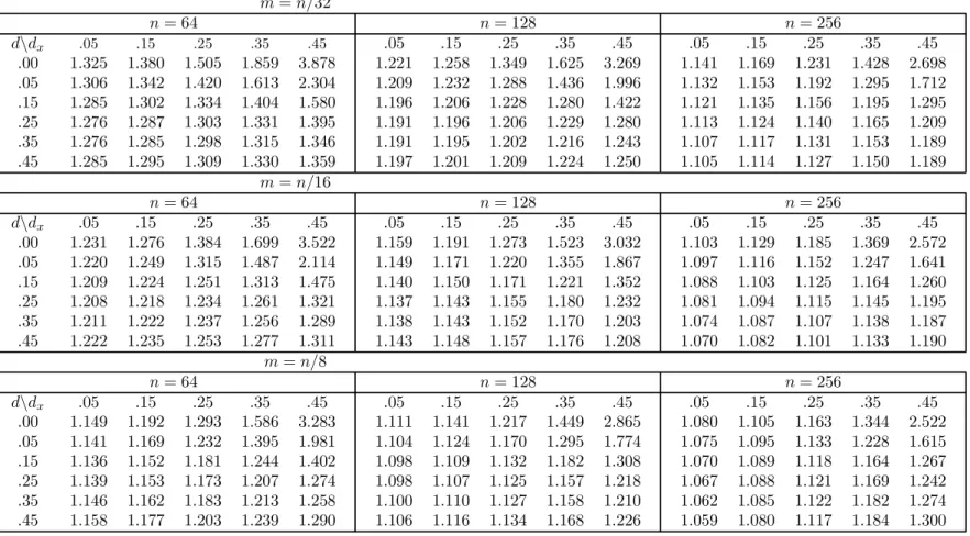
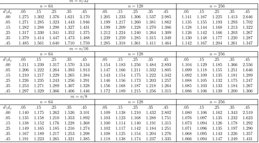
Ω= 1 2π Z π −π ¯ ¯1−eiλ¯¯2(d−dx)dλ= 2 4(d−dx) π B µ d−dx+ 1 2, d−dx+ 1 2 ¶ , where B(·,·) is the Beta function. Almost uniformly, R > 1, with R tending to approach1withnincreasing as expected. For the most part, for givenn R tends to fall with increasingm, the most noticeable exceptions occurring when bothd is small anddx is large, with the variation acrossm not always being monotonic,
such that in some cases an “optimal”m (in the sense that theM SE most closely approximates its limiting value) lies within the range of m employed. It is not surprising that the implications for choice ofmshould vary across d, but perhaps surprising that they should vary across dx. We conjecture that the fact that the
results deteriorate asdx increases when d = 0 is a second order effect due to the
slow convergence of n−1Pnt=1x2t to σ2x when dx ≥ 1/4 (see Rosenblatt, (1961)),
GLSthen being asymptotically equivalent toOLS under our simple model forut;
as d increases it tends to ”compensate” for dx and the effect diminishes. So far
as the comparison between Methods 1 and 2 is concerned, as expected Method 2 performs better for the smaller values of d+dx, whereOLS is n1/2-consistent
(indeed with d = 0 in our model it is efficient), and surprisingly does so also in some cases whend+dx ≥1/2. However, the discrepancies in the former situation
tend to be small, whereas on the occasions where Method1beats Method 2 they are sometimes quite substantial.
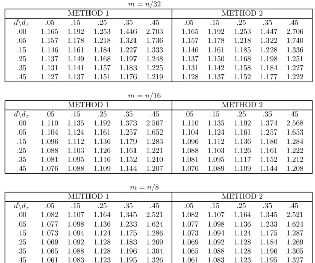
One can iterate theGLS procedures, on each step replacingβe in(2.2) by the current estimate from the previousGLSstep in order to re-estimatef prior to the nextGLS step. Such iterations cannot improve asymptotic first-order efficiency, but might be expected to approach a form of frequency-domain Gaussian pseudo maximum likelihood estimate. Because the iterations tended to settle down after two iterations following the initialGLSestimation (suggesting fairly quick conver-gence), Table 3 contains results forR based on twice iterating either of Methods 1 and 2 (with n = 256). For Method 1, the iterations worsen the M SE ratio in all cases, although in 62 cases out of 90 the discrepancy is smaller than 2%. The relative performance of iteration tended to be even worse for n = 64,128. This behaviour may be due to the fact that the estimate to which the iterations numerically converge is implicitly-defined, and the finite-sample properties of es-timates of this type can sometimes be inferior to those of simpler, closed-form,
estimates. Moreover, in his original paper, Hannan (1963) referred to the pos-sibility of iterating his, related, GLS procedure, but noted ”experience suggests that this would not be worthwhile”. For Method 2, iteration worsens matters in 42 cases out of 90, though by more than 2% in only 6 cases. Note the improve-ments achieved here whend+dx ≥1/2, which is the situation in which the GLS
procedure has not been theoretically justified owing to C9 not holding; the larger d+dx, the better. This appears to illustrate a general result of Robinson (1988),
which indicates that certain iterations can improve anγ-consistent estimate to an n1/2-consistent one, in finitely many steps.
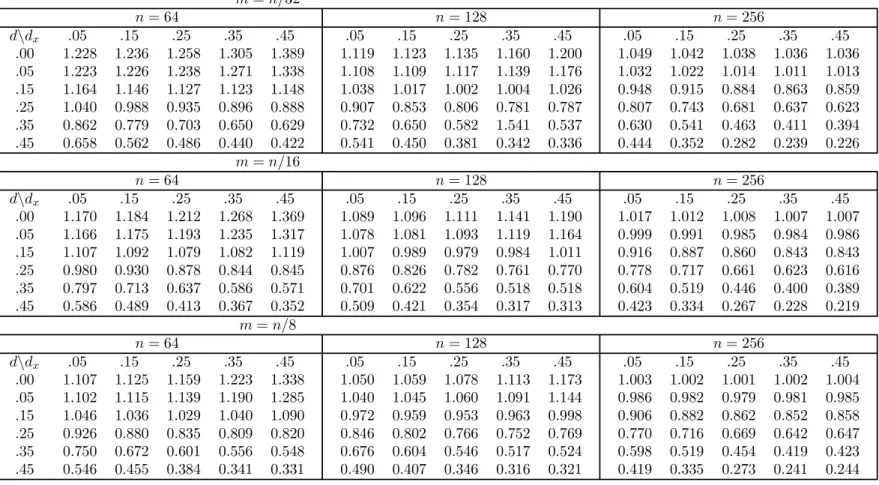
Thefinite sample efficiency ofGLSrelative to the preliminary estimates is also of interest, in view of the extra computation and the bandwidth choice that it requires. For the same model employed in the current simulations, Robinson and Hidalgo (1997) analytically calculated asymptotic efficiency relative to bβϕ under
(2.3) (the preliminary estimate for Method1) over the same(d, dx)grid as in the
present paper. To complement this, and recognize the popularity of OLS, Table 4 reports Monte Carlo efficiency R∗ =M SE(GLS)/M SE(OLS) for the samen, m and parameter values as before, with GLS computed according to Method 2. Notice that whenn= 64GLSis noticeably worse thanOLS for smallishd, due to the imprecision introduced by the nonparametric spectral estimation. This effect diminishes with increasing n, such that with n = 256, R∗ barely exceeds 1 for d= 0, in which case OLS is of course asymptotically efficient. For larger d, even whenn= 64, GLSnoticeably improves upon OLS, with monotonic reduction in R∗ asmdecreases, while there is global improvement inGLS asnincreases. GLS tends to improve with increasing dx, though some evidence of a trough around
dx= 0.35is detected.
4. PROOF OF THEOREM 2.1
Denote Ixx(λj) andfb(λj) byIxx,j andfbj respectively. It suffices to prove that
1 n1/2 n−1 X j=1 b fj−1qj d →N(0,Ω) (4.1) and 1 n n−1 X j=1 b fj−1Ixx,j p →Ω, (4.2)
where qj = wx(λj)w∗u(λj), with wu(λ) = (2πn)−
1/2Pn
t=1uteitλ. We establish
only(4.1), omitting for the sake of brevity the much easier proof of (4.2). Introduce the infeasible estimate off(λ),
ˇ f(λ) = 1 c(2m+ 1) m X j=−m cjIuu(λ+λj),
whereIuu(λ) =|wu(λ)|2and abbreviatef(λj)andfˇ(λj)asfj andfˇjrespectively.
Now(4.1) follows if 1 n1/2 n−1 X j=1 ˇ fj−1qj d →N(0,Ω) (4.3) and 1 n1/2 n−1 X j=1 ³ b fj−1−fˇj−1´qj p →0. (4.4)
A key difficulty in establishing(4.3)and(4.4)is thatfˇj, and its feasible version
b
fj, do not well approximatefj forλj suitably near to zero frequency, wheref(λ)
can have a pole, while dealing withfj itself in this region poses technical difficulty.
The latter problem is dealt with by suitable truncation with respect to frequency, somewhat after the manner of Robinson(1995a, b)in his study of estimating(2.1). For the first, Propositions A.2, A.3 and A.6 deal with behaviour of the centred quantities fˇj −Efˇj, the latter proposition proving the modification of (4.4) in
which the bracketed factor is replaced byfˇj−1−(Efˇj)−1. However,Efˇj does not
approximatefj for small enoughj - Proposition A.1finds that, asm→ ∞withn,
according to C8, it varies likefj forj = 2m+ 1, ...,[n/2], where[.]denotes integer
part, but likefmforj = 1, ...,2m. Whend >0we cannot therefore expect to have
an asymptotically unbiased estimator forfj atj = 1, ...,2m. So the modification
of (4.4) with the bracketed factor replaced by ¡Efˇj
¢−1
−f 1
j needs special care
for these frequencies. Nevertheless, because the latter form an asymptotically negligible fraction of the Fourier frequencies used in the estimation, Proposition A.4 is able to show that the error thereby included is asymptotically negligible.
However, the latter requiresm=o¡n1/2¢, under the mild Condition C4, as can be observed from Lemma B.7. On the other hand, sincebβfb−1 involves thefbj as
ran-dom denominators, then as in other semiparametric estimation problems, uniform convergence of thefbj is required. Following, for instance, Brillinger(1981, p.445),
whose approach is employed in the proof of Proposition A.3, we can expect the rate of such uniform convergence to be Op
¡
nm−k¢ when Eu4tk < ∞. So, the
latter order of magnitude, together with our condition m=o¡n1/2¢, implies that
for uniform convergence we need k ≥ 3, that is finite 12th moments. Although 13
Lemma B.7 indicates that the 12th moment condition on ut could be relaxed,
this is possible only at the expense of strengthening other conditions, notably Conditions C4 and C8. More specifically, allowing F(λ)−F (0) = O¡λ1−2dx¢,
or alternatively Γ(j) = O¡j2dx−1¢, with d
x < 1/2, implies that we can choose
m=O¡n(1+δ)/2¢ for 0<δ <1/3. However, this would require strengthening the
weak Condition C4. So, we have preferred to keep Condition C2 as it stands since from the aforementioned result of Brillinger, we would in any case needutto have
finite 8th moments.
The remainder of the proof is mainly concerned with showing that fb can replace fˇ, see (4.4). Though condition C9 plays a major role here, the proof is considerably more complex than the corresponding parts of the proofs of Hannan (1963), Robinson (1991), due to the allowance for long memory in ut and xt.
In particular, care is needed in dealing with fact that discrete Fourier transforms behave differently close to zero frequency than they do far from it. The remainder of the current section deals principally with this matter of proving (4.4), but we first establish (4.3), whose left side is
1 n1/2 n−1 X j=1 fj−1qj + 1 n1/2 n−1 X j=1 ³ ˇ fj−1−¡Efˇj ¢−1´ qj + 1 n1/2 n−1 X j=1 ³¡ Efˇj ¢−1 −fj−1´qj. (4.5) The second and third terms of(4.5)areop(1)by Propositions A.6 and A.4
respec-tively of Appendix A, while thefirst term converges in distribution toN(0,Ω)by the proof of Theorem1of Robinson and Hidalgo (1997). Thus (4.3) is proved.
We now prove (4.4). By the Schwarz inequality the left side of (4.4) has squared modulus bounded by
Ãn−1 X j=1 ¯ ¯ ¯¡Efˇj ¢−1³ˇ fj−fbj´¯¯¯ 2¯¯ ¯ bfj−1¡Efˇj ¢2 ˇ fj−1¯¯¯2 ! à 1 n n−1 X j=1 ° ° °¡Efˇj ¢−1 qj ° ° °2 ! , (4.6)
where k·k denotes the Euclidean norm, and the presence of the factors Efˇj and
its reciprocal is due to remarks above. Letnbe so large that2m <[n/2]. Writing aj,n =
¡ Efˇj
¢−1
fj, the expectation of the second bracketed factor of (4.6)is
2 n 2m X j=1 E ° ° ° °aj,n qj fj ° ° ° ° 2 + 2 n [n/2] X j=2m+1 E ° ° ° °aj,n qj fj ° ° ° ° 2 .
The first term is O(1) by Lemma B.7 since by Proposition A.1 part (a) K−1 <
¯ ¯λ2md
¡
Efˇj¢¯¯ < K, where K henceforth denotes an arbitrarily large but finite
positive constant, and by C1 fjλ2md ≤ K(m/j)
2d
|aj,n| ≤ K(m/j)
2d
. The second term of the last displayed expression is also O(1) as we now show. By Proposition A.1 parts (b) and(c), |aj,n−1| ≤Km/j,
so that term is bounded by K n [Xn/2] j=2m+1 ¡ 1 +mj−1¢2E ° ° ° °qfjj ° ° ° ° 2 ≤ K n [n/2] X j=2m+1 E¡fj−1Iuu,j ¢ tr(E(Ixx,j)) ≤ Kn [n/2] X j=2m+1 tr(E(Ixx,j)) =O(1)
where thefirst inequality follows by C5 and the fact thatfj−1 ≤K (by C1and C3),
and the second inequality from Robinson’s(1995a)Theorem 2, E¡fj−1Iuu,j
¢
≤K andP[jn/=22]m+1EIxx,j ≤(2π)−1Pnj=1Extx0t=O(n).
Thus, by Markov’s inequality, the second factor of (4.6) is Op(1), and the
proof of the Theorem is completed if the first factor of (4.6) is op(1). We prove
below that n−1 X j=1 ¯ ¯ ¯¡Efˇj ¢−1³ˇ fj−fbj´¯¯¯ 2 = op(1), (4.7) sup j=1,...,[n/2] ¯ ¯ ¯¡Efˇj ¢−1 b fj−1 ¯ ¯ ¯ = op(1). (4.8)
In addition, by Propositions A.1 and A.3, sup j=1,...,[n/2] ¯ ¯ ¯¡Efˇj ¢−1 ˇ fj −1 ¯ ¯ ¯=op(1). (4.9)
The proof then follows in the same spirit as in Hannan (1963), see also Hannan (1970, p.489). By(4.8)and(4.9), ¯ ¯ ¯¡Efˇj ¢−1 b fj ¯ ¯ ¯≥ K−1 >0 and ¯ ¯ ¯¡Efˇj ¢−1 ˇ fj ¯ ¯ ¯≥K−1 >0 (4.10) with probability approaching one as n → ∞. The first factor of (4.6) is thus bounded by sup j=1,...,[n/2] ¯ ¯ ¯ bfj ¡ Efˇj ¢−2 ˇ fj ¯ ¯ ¯−2 n−1 X j=1 ¯ ¯ ¯¡Efˇj ¢−1³ˇ fj−fbj´¯¯¯ 2 ≤ K n−1 X j=1 ¯ ¯ ¯¡Efˇj ¢−1³ˇ fj −fbj´¯¯¯ 2 = op(1),
using(4.7), so the first factor of(4.6), and thus the left side of (4.4), is op(1).
It remains to prove(4.7) and(4.8). We begin with(4.7). By (1.1) b fj −fˇj = 2 ³ e β−β ´0 bj + ³ e β−β ´0 Bj ³ e β−β ´ , (4.11)
where, denotingRe (z)as the real part of the complex number z, bj = 1 c(2m+ 1) X `(j) 0 c`Re (qj+`), Bj = 1 c(2m+ 1) X `(j) 0 c`Ixx,j+`,
in which P`(j)0 = Pm`=−m,`+j6=0. Notice that the exclusion of the non-mean-corrected quantities qj+`, Ixx,j+` for j +` 6= 0 corresponds to the sample-
mean-correction in(2.2).
Noting that, by boundedness of thec` and periodicity of Ixx(λ),
kBjk≤ K mtr µPn k=1 Ixx,k ¶ ≤ Kmtr µPn t=1 xtx0t ¶ =Op ³n m ´ (4.12) uniformly inj, whereas n P j=1k Bjk≤ Ktr µ n P k=1 Ixx,k ¶ =Op(n),
the contribution to(4.7)due to the final term of (4.11) is bounded by ° ° °eβ−β ° ° ° 4nP−1 j=1 ¡ Efˇj ¢−2 kBjk2 ≤K ° ° °eβ−β ° ° ° 4 sup j k Bjk n P j=1k Bjk=Op µ 1 m ¶ , since ¡Efˇj ¢−1
≤K by Proposition A.1 in Appendix A and C9 holds. Next, the contribution to(4.7)due to bj in(4.11) is bounded by
4n ° ° °eβ−β ° ° °2 [n2/3] X j=1 ° ° °¡Efˇj ¢−1 n−1/2bj ° ° °2+ [n/2] X j=1+[n2/3] ° ° °¡Efˇj ¢−1 n−1/2bj ° ° °2 . (4.13) By elementary inequalities thefirst sum on (4.13) is bounded by
K m2 2m X j=1 ° ° ° ° ° ° 1 n1/2 X `(j) 0 c`λ2mdRe (qj+`) ° ° ° ° ° ° 2 + K m2 [n2/3] X j=2m+1 ° ° ° ° ° ° 1 n1/2 X `(j) 0 c`fj−+1`Re (qj+`) ° ° ° ° ° ° 2 , (4.14) because ¡Efˇj ¢−1
≤ Kλ2md for 1 ≤ j ≤ 2m by Proposition A.1 part (a) and ¡
Efˇj
¢−1
for1≤j ≤2m andj+` 6= 0, we have f|j+`|λ2md< K(m/|j+`|)
2d
, so by Lemma B.7 the expectation of the first term of (4.14) is bounded by
K m2 2m X j=1 1 =O µ 1 m ¶ =o(1),
using C8, whereas the second term of(4.14) has expectation bounded by K m2 [n2/3] X j=2m+1 1 =O µ n2/3 m2 ¶ =o(1),
using C8 and proceeding as in the proof of the first term on the right of (B.11) but taking the weights aj,n there to be bounded byK.
Now consider the second sum on the right of(4.13). Letwε,j = (2πn)−1/2Pnt=1εteitλj.
By elementary inequalities andRe (qj+`) =
¡
qj+`+qj∗+`
¢
/2, that sum is bounded by Kn−1 [Xn/2] j=1+[n2/3] ° ° ° ° ° ° 1 (2m+ 1) X `(j) 0 c` fj1+/2` ¡ Efˇj ¢ Ã wu,j+` fj1+/2` − (2π)1/2wε,j+` σ ! w∗x,j+` ° ° ° ° ° ° 2 +Kn−1 [n/2] X j=1+[n2/3] ° ° ° ° ° ° 1 (2m+ 1) X `(j) 0 c` fj1+/2` ¡ Efˇj ¢wε,j+`wx,j∗ +` ° ° ° ° ° ° 2 . (4.15)
Because by C1and C3 and Proposition A.1parts (b) and(c)¡Efˇj
¢−1
≤Kfj−1 ≤ Kfj−+1`/2, and because Ewε,j+`w∗ε,k+` = (σ2/2π)I(j =k) by C2, see Brillinger
(1981, Exercise 4.8.12), the expectation of the second term of(4.15) is K n [Xn/2] j=1+[n2/3] 1 (2m+ 1)2 X `(j) 0 c2`tr{EIxx,j+`} ≤ K nm2 [Xn/2] j=1+[n2/3] m X `=−m tr{EIxx,j+`} ≤ K nm [Xn/2] j=1+[n2/3] tr{EIxx,j}=O ¡ m−1¢,
since the sum is bounded byPnj=1−1EIxx,j = (2π)−
1Pn
t=1E(xtx0t) =O(n). On the
other hand, by the Schwarz inequality the expectation of the first term of (4.15)
is bounded by K nm2 [Xn/2] j=1+[n2/3] m X `=−m E ¯ ¯ ¯ ¯ ¯ wu,j+` fj1+/2` − (2π)1/2wε,j+` σ ¯ ¯ ¯ ¯ ¯ 2 m X `=−m tr{EIxx,j+`} ≤ nmK2 [Xn/2] j=1+[n2/3] m X `=−m log (j +`) j+` m X `=−m tr{EIxx,j+`}=O µ log2n m 
by Robinson’s (1995a) Theorem 2, Pn`=1`−1log` = O¡log2
n¢ and proceeding as in the proof of the second term of (4.15). Thus from C9 (4.13) is op(1), to
complete the proof that(4.7) isop(1).
Finally consider (4.8). By the triangle inequality the left side of (4.8) is bounded by sup j ¯ ¯ ¯¡Efˇj ¢−1³ˇ fj −fbj´¯¯¯+ sup j ¯ ¯ ¯¡Efˇj ¢−1¡ˇ fj −E ¡ˇ fj¢¢¯¯¯.
The second term isop(1)by(4.9), whereas, by the triangle inequality and(4.11),
thefirst term is bounded by 2°°°eβ−β°°°sup j ° ° °¡Efˇj ¢−1 bj ° ° °+°°°eβ−β°°°2¡Efˇj ¢−1 sup j k Bjk. (4.16)
The second term of (4.16) is op(1) because of C9, (4.12) and Proposition A.1,
whereas thefirst term is bounded by ° ° °eβ−β ° ° ° 2[Xn/2] j=1 ° ° °¡Efˇj ¢−1 bj ° ° ° 2 1/2 =op(1)
since we have already shown that (4.13) = op(1). This concludes the proof of
(4.8) and the theorem. ¤
APPENDIX A
Ourfirst proposition is concerned with the asymptotic behaviour ofEfˇj across
three suitably chosen, exhaustive subsets of the Fourier frequencies. We find it convenient to approximateEfˇj, over two of these subsets, by
e fj = 1 c(2m+ 1) X `(j) 0 c`fj+`, 1≤j ≤[n/2]; fej =fen−j, 1 + [n/2]≤j < n,
whose varying orders of magnitude are indicated in the proposition. We shall then employ fej subsequently in the proposition, largely as abbreviating notation for
these orders of magnitude.
Proposition A.1 Let C1-C3 and C7-C8 hold. Then as n → ∞,
(a) sup 1≤j≤2m ¯ ¯ ¯λ2dm ³E¡ˇfj ¢ −efj´¯¯¯=O µ logm m1−2d ¶ , where K−1 ≤ ¯ ¯ ¯λ2dmefj ¯ ¯
¯≤K for j =1, ...,2m, independently of j and n. (b) For arbitrarily small δ >0,
sup 2m<j≤[δn/2] ¯ ¯ ¯fj−1 ³ E¡ˇfj ¢ −efj´¯¯¯=O µ logm m ¶ , where K−1≤¯¯¯fj−1efj ¯ ¯ ¯≤K for j =2m +1, ...,[n/2] and supj=2m+1,...,[n/2](j/m) ¯ ¯ ¯fj−1efj−1 ¯ ¯ ¯=O(1)as n → ∞. (c) For arbitrarily small δ >0, as n → ∞,
sup [δn/2]<j≤[n/2] ¯ ¯E ¡ˇfj ¢ −fj¯¯=O³m n ´ .
Proof. Wefirst prove (a). By definition E¡fˇj ¢ −fej = 1 c(2m+ 1) X `(j) 0 c`{EIj+`−fj+`},
abbreviating Iuu,j as Ij. By C7 and Theorems 1 and 2 of Robinson (1995a), see
in particular his(4.2), the right side of the last displayed equation is bounded in absolute value by K m m X `=−m 06=|j+`|≤r fj+`+ K m m X `=−m r<|j+`| fj+` µ log|j+`| |j+`| ¶ ≤ Krm r X `=1 f`+ Klogm m 2m X `=r+1 `−1f`,
for somer >0. (Observe that the component |(j +`)/n|η in Robinson’s (1995a) Theorem 2 does not appear since we employ fj+` instead of its approximation
Cλ−j+2`d.) By C1, and with r = log1/2m, the right side of the last displayed in-equality is bounded by Klogm m 2m X `=1 `−1λ−`2d=O¡(logm)λ−m2d/m1−2d ¢ . To complete the proof of part (a) we need to show that K−1
≤ ¯¯¯λ2mdfej
¯ ¯
¯ ≤ K. First,λ2mdfej has absolute value upper-bounded by
Km2d−1
2m
X
`=1
`−2d≤K,
whereas, by C7 and forn sufficiently large,min[m/4]≤`≤[m/2]c` > K−1, so
¯ ¯ ¯λ2mdfej ¯ ¯ ¯≥K−1m2d−1 [Xm/2] `=[m/4] (j+`)−2d≥K−1.
Now consider part (b). By definition of fj−1³E¡fˇj
¢
−fej
´
and triangle in-equality we have ¯ ¯ ¯fj−1 ³ E¡fˇj ¢ −fej´¯¯¯≤fj−1 1 c(2m+ 1) m X `=−m c`|E(Ij+`)−fj+`|,
which, by Theorem 2 of Robinson(1995a)and its routine extension for2m < j < [nδ/2] with arbitrarily smallδ>0, is bounded by
fj−1 K (2m+ 1) m X `=−m fj+` ¯ ¯ ¯ ¯ log (j+`) j+` ¯ ¯ ¯ ¯=O¡m−1logm¢, because |log (j +`)/(j+`)| = O(m−1logm) and f−1
j fj+` ≤ K by C1 and C3
uniformly in` for all2m < j ≤[nδ/2]. We provefinally thatK−1
≤ ¯ ¯ ¯fj−1fej ¯ ¯ ¯≤K. By C1, ¯ ¯ ¯fj−1fej ¯ ¯ ¯≤ Km m X `=−m ¯ ¯ ¯ ¯ffj+j` ¯ ¯ ¯ ¯≤ Km m X `=−m ¯ ¯ ¯ ¯j+j ` ¯ ¯ ¯ ¯ 2d ≤K,
because for j > 2m and |`| ≤ m, we have 2−1 < |1 +`/j|. On the other hand, proceeding as in part(a)
¯ ¯ ¯fj−1fej ¯ ¯ ¯≥K−1m−1 [m/2] X `=[m/4] ¯ ¯ ¯ ¯j+j ` ¯ ¯ ¯ ¯ 2d ≥K−1,
because forj >2m and|`|≤m, |1 +`/j|<3/2. Next we show that sup2m<j≤[n/2](j/m) ¯ ¯ ¯fj−1fej−1 ¯ ¯ ¯=O(1) asn→ ∞. By definition µ j m ¶ ¯¯ ¯fj−1fej−1 ¯ ¯ ¯ = µ j m ¶ 1 c(2m+ 1) ¯ ¯ ¯ ¯ ¯ m X `=−m c` µ fj+` fj − 1 ¶¯¯¯ ¯ ¯ ≤ µ j m ¶ K (2m+ 1) m X `=−m |`| j ≤K (A.1)
by the mean value theorem and triangle inequality, so that thesup2m<j≤[n/2]
¡j m¢ ¯¯¯f −1 j fej−1 ¯ ¯ ¯= O(1). This concludes the proof of part (b).
Finally we prove (c). First, by definition E¡fˇj ¢ −fj = 1 c(2m+ 1) m X `=−m c`(E(Ij+`)−fj+`) + 1 c(2m+ 1) m X `=−m c`(fj+`−fj). (A.2)
Because[δn/2]< j ≤[n/2]andf(λ)is continuously differentiable forδ<|λ|≤π by C3, the second term on the right of(4.2) is bounded by
K (2m+ 1) m X `=−m c`| `| n (1 +o(1)) =O ³m n ´ .
Finally, thefirst term on the right of(A.2)isO(n−1logn)by an obvious extension of the proof of Robinson’s(1995a)Theorem 2 to0<δ ≤|λ|≤π. This concludes
the proof of part (c) and of the Proposition. ¤
Proposition A.2 Assuming C1-C3 and C7-C8, as n → ∞ efj−2Cov ¡ˇfj,ˇfj ¢ = ½ O(m−1) if 2m < |j|≤[n/2] O(g(m)) if 1 ≤|j|≤2m, where g(m) =m4d−2 I(d >1/4) +m−1logm I(d =1/4) +m−1 I(d <1/4).
Proof. We begin by estimating Cov¡fˇj,fˇj
¢ , which is 1 4π2n2c2(2m+ 1)2 X `(j) 0 X k(j) 0 c`ck X t1, X t2, n X t3, X t4=1 © γt1−t3γt2−t4 +γt1−t4γt2−t3 +cum(ut1, ut2, ut3, ut4)}e i(t1−t2)λ`+j−i(t3−t4)λk+j. (A.3)
We deal only with the contributions from thefirst and third terms in braces, that from the second being handled similarly to thefirst. Applying Brillinger
(1981, (2.6.3) p. 26, and (2.10.3) p. 39), the contribution from the third term of(A.3) is bounded in absolute value by
K n2(2m+ 1)2 X `(j) 0 X k(j) 0 c`ck ¯ ¯ ¯ ¯ Z [−π,π]3 τ(−λ)τ(−µ)τ(−ζ)τ(λ+µ+ζ) ×D(λ+λ`+j)D(µ−λ`+j)D(ζ−λk+j)D(λk+j −(λ+µ+ζ))dλdµdζ| = K n2(2m+ 1)2 X `(j) 0 X k(j) 0 c`ck|τ(λ`+j)τ(−λ`+j)τ(λk+j)τ(−λk+j) (A.4) × Z [−π,π]3 τ(−λ)τ(−µ)τ(−ζ)τ(λ+µ+ζ) τ(λ`+j)τ(−λ`+j)τ(λk+j)τ(−λk+j) ×D(λ+λ`+j)D(µ−λ`+j)D(ζ−λk+j)D(λk+j−(λ+µ+ζ))dλdµdζ|,
where D(w) = Pn`=0−1e−i`w is the Dirichlet kernel and we note that f(λ) > 0 implies that|τ(λ)|>0. Because
Z
[−π,π]3
D(λ+λ`+j)D(µ−λ`+j)D(ζ−λk+j)D(λk+j −(λ+µ+ζ))dλdµdζ = (2π)
3
n, using the identity
q1q2q3q4 = (q1q2−1) (q3q4−1) + 2 X `=1 (q2`−1 −1) (q2`−1) + 4 X i=1 (qi−1) + 1,
and proceeding as in the proof of (4.28) in Robinson (1995b), the right side of (A.4) is bounded by K (2m+ 1)2 X `(j) 0 X k(j) 0 c`ckf`+jfk+j ¡ n−1+|`+j|−1|k+j|−1 (A.5) +|`+j|−1/2|k+j|−1 +|`+j|−1|k+j|−1/2+n−1/2|`+j|−1/2|k+j|−1/2´,
since ¯ ¯ ¯f`−+1j/2τ(λ`+j) ¯ ¯ ¯< K.
Next, we examine thefirst term of (A.3), which can be written 1 4π2n2c2(2m+ 1)2 X `(j) 0 X k(j) 0 c`ck ½Z D(θ)D(λk−`−θ)f(θ+λ`+j)dθ × Z D(−θ)D(θ+λ`−k)f(θ−λk+j)dθ ¾ . (A.6)
We study the first term inside the braces of (A.6), the second being identical. Adding and subtractingf`+j
R D(θ)D(λk−`−θ)dθ, this term is Z D(θ)D(λk−`−θ) (f(θ+λ`+j)−f`+j)dθ+f`+j Z D(θ)D(λk−`−θ)dθ.
By Theorem 2 of Robinson(1995a), the first term of this expression is
O(n(log|k+j|)f`+j/|`+j|), whereas the second term is zero unless k = `, in
which case it is2πnf`+j. Thus, as n→ ∞, the modulus of (A.6)is bounded by
K (2m+ 1)2 X `(j) 0 X k(j) 0 c`ckf`+jfk+j log2|k+j| |`+j| |k+j| + K (2m+ 1)2 X `(j) 0 c2`f`2+j µ log|`+j| |`+j| + 1 ¶ . (A.7)
Similarly, the second term of (A.3) is, as n→ ∞, bounded by K (2m+ 1)2 X `(j) 0 X k(j) 0 c`ckf`+jfk+j log2|k+j| |`+j| |k+j| + K (2m+ 1)2 X `(j),k(j) 00 c`ckf`+jfk+j µ log|`+j| |`+j| + 1 ¶ , (A.8)
where P`(j),k(j)00 denotes the terms in the double sum P`(j)0 Pk(j)0 such that k+`+ 2j = 0. Thus,
¯
¯Cov¡fˇj,fˇj¢¯¯≤(A.5) + (A.7) + (A.8). (A.9)
We now turn to the proof for 2m < |j| ≤ [n/2]. Applying Lemma B.1 with ψ = 0,1/2,1, the first term on the right of (A.9) is O¡m−3/2f2
j
¢
by C8. Next, consider the second term on the right of (A.9), namely (A.7). Its first term is bounded by Klog 2 |j| j2 1 (2m+ 1) X `(j) 0 c`f`+j 2 =O µ log2|j| j2 f 2 j ¶ , 23
from Lemma B.1 with ψ= 0. The second term of(A.7) is dominated by K 1 m2 X `(j) 0 c2`f`2+j =O¡m−1fj2¢,
because by the mean value theoremfj−2
¯ ¯f`2+j −fj2 ¯ ¯≤K(`/j)< K for 2m < j ≤ [n/2], so f`2+j =O ¡ fj2 ¢
and thus (A.7)is O¡m−1fj2
¢ .
The third term on the right of (A.9) (that is, (A.8)) is, proceeding as with (A.7), O¡m−3/2fj2
¢
, by C8 and the fact that, for j >2m, the last term of (A.8) is zero. Thus, we conclude that (A.3) is O¡m−1fj2
¢
and that fej−2Cov¡fˇj,fˇj
¢ = O(m−1), since by Proposition A.1 parts (b) and(c), fej−2 =O¡fj−2¢.
Next, for 1 ≤ |j| ≤ 2m. Using Lemma B.2 instead of Lemma B.1, it is straightforward to observe that(A.9) is
O¡n4dm−2¡m1−4dI(d <1/4) + logmI(d = 1/4) +I(d >1/4)¢¢.
But by Proposition A.1 part (a),fej−2 =O¡λ4md¢, which concludes the proof. ¤
Proposition A.3 Let C1-C3, C7 and C8 hold. Then, as n → ∞,
(a) sup j=1,...,2m ¯ ¯ ¯efj−1¡ˇfj−Eˇfj¢¯¯¯=op(1) (b) sup j=2m+1,...,k ¯ ¯ ¯efj−1¡ˇfj−Eˇfj¢¯¯¯=Op ³ k1/6/m1/2´.
Proof. Wefirst show (b). Observing that by triangle inequality, sup j=2m+1,...,k ¯ ¯ ¯ efj ¡ˇ fj−Efˇj¢¯¯¯≤ sup j=2m+1,...,k ¯ ¯ ¯ efjh1j ¯ ¯ ¯+ sup j=2m+1,...,k ¯ ¯ ¯ efjh2j ¯ ¯ ¯ where h1j = 1 2m+ 1 X `(j) 0 c`f`+j ½µ I`+j f`+j − 2πIεε,`+j σ2 ¶ − µ E(I`+j) f`+j − 1 ¶¾ (A.10) and h2j = 1 2m+ 1 X `(j) 0 c`f`+j µ 2πIεε,`+j σ2 −1 ¶ , (A.11)
the proof of(b)is in two parts. Since ¡supj|aj|
¢υ ≤Pj|aj| υ , wefirst show that µ sup j=2m+1,...,k ¯ ¯ ¯ efjh1j ¯ ¯ ¯ ¶2 ≤ k X j=2m+1 ¯ ¯ ¯ efjh1j ¯ ¯ ¯2 =Op µ log2k m ¶ (A.12)
and then that µ sup j=2m+1,...,k ¯ ¯ ¯ efjh2j ¯ ¯ ¯ ¶6 ≤ k X j=2m+1 ¯ ¯ ¯ efjh2j ¯ ¯ ¯6 =Op µ k m3 ¶ . (A.13)
Using the inequality in(A.12), and that(a+b)2 ≤2a2+2b2,³sup
j=2m+1,...,k ¯ ¯ ¯ efjh1j ¯ ¯ ¯´2is bounded by 2 k X j=2m+1 e fj−2 1 2m+ 1 X `(j) 0 c`f`+j µ I`+j f`+j − 2πIεε,`+j σ2 ¶ 2 (A.14) +2 k X j=2m+1 e fj−2 1 2m+ 1 X `(j) 0 c`f`+j µ E(I`+j) f`+j − 1 ¶ 2 .
But proceeding step-by-step as in the proof of (4.8) in Robinson (1995b), the expectation of thefirst term of(A.14) is bounded by
K m2 k X j=2m+1 e fj−2fj2 m X `=−m µ f`+j fj ¶2 log (`+j) `+j ≤ K m2 m X `=−m log2k=O¡m−1log2k¢, because¯¯fj−1f`+j ¯ ¯≤K by C1 and C3 and ¯ ¯ ¯ efj−1fj ¯ ¯ ¯≤K by Proposition A.1 parts (b)and(c). Next, using Robinson’s(1995a)Theorem 2 and its obvious extension for allj = 2m+ 1, ...,[n/2], the second term of (A.14) is bounded by
K k X j=2m+1 ¯ ¯ ¯ ¯ ¯fe −1 j 1 2m+ 1 m X `=−m c`f`+j log (`+j) `+j ¯ ¯ ¯ ¯ ¯ 2 ≤K k X j=2m+1 ¯ ¯ ¯ ¯fej−1fj logk (j−m) ¯ ¯ ¯ ¯ 2 =O µ log2k m ¶ ,
applying Lemma B.1with ψ = 0, and using the fact that supj=2m+1,...,k
¯ ¯ ¯ efj−1fj ¯ ¯ ¯≤
K by Proposition A.1parts (b)and(c). Next, using the inequality in (A.13), the expectation of³supj=2m+1,...,k ¯ ¯ ¯ efj−1h2j ¯ ¯ ¯´6 is bounded by k X j=2m+1 e fj−6fj6E ¯ ¯ ¯ ¯ ¯ 1 2m+ 1 m X `=−m c` µ f`+j fj ¶ µ 2πIεε,`+j σ2 −1 ¶¯¯¯ ¯ ¯ 6 =O¡km−3¢
from the proof of Brillinger’s(1981) Theorem 7.4.4., and supj=2m+1,...,k
¯ ¯ ¯ efj−1fj ¯ ¯ ¯≤
K and |f`+j/fj|≤K, as argued above. This concludes the proof of part (b).
To prove part(a), wefirst consider the cased≥1/4. Writeχj =fej−1 ¡ˇ fj−Efˇj ¢ andeγr=bγr−Ebγr, wherebγr=n−1Pn−|r| t=1 utut+|r|. By direct calculation, ¯ ¯χj¯¯2 = ¯ ¯ ¯ ¯ ¯ ¯ 1 e fjc(2m+ 1) X `(j) 0 c`(I`+j −E(I`+j)) ¯ ¯ ¯ ¯ ¯ ¯ 2 = ¯ ¯ ¯ ¯ ¯ 1 2πfejc n−1 X r=1−n Cj(r)eirλjeγr ¯ ¯ ¯ ¯ ¯ 2 , (A.15) where Cj(r) = 1 (2m+ 1) X `(j) 0 c`eirλ`. (A.16) Notefirst that sup j=1,...,2m ¯ ¯χj¯¯2 ≤Kλ4md sup j=1,...,2m ¯ ¯ ¯ ¯ ¯ n−1 X r=1−n Cj(r)eirλjeγr ¯ ¯ ¯ ¯ ¯ 2
by definition of fej and χj in (A.15) and by Proposition A.1 part (a). By the
Schwarz inequality, the right side of the last displayed inequality is bounded by ¡ Kλ4md ¢ sup j=1,...,2m ¯ ¯ ¯ ¯ ¯ n−1 X r=1−n |Cj(r)| ¯ ¯ ¯ ¯ ¯j=1sup,...,2m ¯ ¯ ¯ ¯ ¯ n−1 X r=1−n |Cj(r)|eγ2r ¯ ¯ ¯ ¯ ¯. The second factor isO(m−1n)by Lemma B.4, whereas the third factor is
Op
¡
m−1n¡n4d−2
I(d≥1/4) +n−1logn
I(d= 1/4)¢¢ by the properties of eγ2r es-tablished in Lemma B.5. The conclusion is now immediate since d <1/2.
To complete the proof we are left with the case d < 1/4. The proof pro-ceeds step-by-step as in part (b), noting that k there is now 2m, fej−1f`+j =
O³m2d/
|`+j|2d´andm4d−1 =o(1)asd <1/4. ¤
For the remaining propositions, let qj and wx,j denote typical components of
the p×1 vectors Ixu,j and wx(λj) respectively, while F (λ) and Γ(s) will here
denote the spectral distribution and autocovariance function of the corresponding element ofxt.
Proposition A.4 Assuming C1-C5 and C7-C8, as n → ∞,
1 n1/2 [n/2] X j=1 " 1 fj− 1 E¡ˇfj ¢ # qj p →0.
Proof. The left side of the above expression is 1 n1/2 [n/2] X j=2m+1 " 1 fj − 1 E¡fˇj ¢ # qj− 1 n1/2 2m X j=1 1 E¡fˇj ¢qj + 1 n1/2 2m X j=1 1 fj qj. (A.17)
The third term of(A.17)isop(1)on takingaj,n = 1for alljin Lemma B.7 since C8
entailsm/n→0and thusF ³λ1m/2
´
−F (0)→0, F(·) being continuous from the right. Now consider the second term of (A.17). Because aj,n = fj
¡ E¡fˇj
¢¢−1
≤
K(m/j)2dby Proposition A.1part(a), it follows from Lemma B.7 that the second term of(A.17) is alsoop(1). Finally the first term of(A.17) is
1 n1/2 [n2/3/logm] X j=2m+1 aj,n 1 fj qj+ 1 n1/2 [n/2] X j=1+[n2/3/logm] aj,n 1 fj qj, (A.18) where aj,n = E¡fˇj ¢ −fj fj 1 fj−1E¡fˇj ¢.
The first term of (A.18) isop(1) as we now show. Since by Proposition A.1part
(b), sup 2m<j≤[δn/2] ¯ ¯ ¯fj−1³E¡fˇj ¢ −fej´¯¯¯=O ¡ m−1logm¢, K−1 < sup 2m<j≤[n/2] ¯ ¯ ¯fj−1fej ¯ ¯ ¯< K, it follows thatK−1 < f−1 j E ¡ˇ fj ¢
< K as n→ ∞, and, using (A.1) for 2m < j ≤ £ n2/3/logm¤, that |aj,n|≤K ¯ ¯ ¯E¡fˇj ¢ −fej ¯ ¯ ¯ fj + ¯ ¯ ¯ efj−fj ¯ ¯ ¯ fj ≤K µ logm m + m j ¶ ≤K µ m j ¶2d
since d < 1/2 and C8 holds. Now proceed as with the second term of (A.17) to conclude that thefirst term of(A.18) is op(1) by Lemma B.7.
Finally consider the second term of (A.18). By Proposition A.1parts (b)and (c) and(A.1) sup [n2/3/logm]<j≤[n/2] ¯ ¯ ¯fj−1fej−1 ¯ ¯ ¯=O µ logm µ m n2/3 + 1 m ¶¶ , so thatsup[n2/3/logm]<j≤[n/2]
¯ ¯a2j,n
¯
¯≤K¡¡m2/n4/3+ 1/m2¢log2m¢≤K¡¡m2log2m¢/n4/3¢. Thus by Lemma B.6 and C8, the second term of(A.18) isop(1)sinced <1/2. ¤
The next Proposition is highly technical and only used in some steps of Propo-sition A.6.
Proposition A.5 Assume C1-C8, and let aj,n be an array of positive bounded
constants. Then, as n → ∞,for k =1,2, 1 n1/2 [n/2] X j=2m+1 aj,nefj−kh k 2j wε,j fj1/2w ∗ x,j=op(1).
Proof. We deal only with the casek = 2, the case k= 1being similarly handled. By definition of h2j given in(A.11), the left side of the last displayed equation is
4π2 σ4(2m+ 1)2n1/2 m X `1,`2=−m [n/2] X j=2m+1 c`1c`2aj,n f2 j e f2 j µ f`1+j fj f`2+j fj ¶ (Iεε,`1+j−EIεε,`1+j) (Iεε,`2+j −EIεε,`2+j) wε,j fj1/2w ∗ x,j. Denote dj = (2πn) 1/2 wε,j. Since fj−1(f`1+j +f`2+j) < K for j > 2m, f −1 j < K by C1 and C3, K−1 < f−1
j fej < K by Proposition A.1 parts (b) and (c) and
¯ ¯a2j,n
¯
¯< K, the variance of the last displayed expression is bounded by K m4n6 m X `i=−m,i=1,...,4 [Xn/2] j1,j2=2m+1 ¯ ¯E¡wx,j∗ 1wx,j2¢¯¯ (A.19) ׯ¯cum¡d`1+j1d∗`1+j1d`2+j1d∗`2+j1dj1, d`3+j2d∗`3+j2d`4+j2d∗`4+j2d ∗ j2¢¯¯ = K m4n6 X v m X `i=−m,i=1,...,4 [n/2] X j1,j2=2m+1 ¯ ¯E¡wx,j∗ 1wx,j2¢¯¯ q Y l=1 |cum(ds1+s2; (s1, s2)∈vl)|
withs1 = 0, `1, `2, `3, `4 ands2 =j1, j2, and where the summation in v is over all
indecomposable partitionsv=v1∪...∪vq, q= 1, ...,5, of the table
d`1+j1 d∗`1+j1 d`2+j1 d∗`2+j1 dj1 d`3+j2 d∗`3+j2 d`4+j2 d∗`4+j2 d
∗
j2,
(A.20) see Brillinger(1981, p.20 and Theorem 2.6.1).
We shall now show that the right side of(A.19) is o(1). When q = 1,2 or 3, using Brillinger’s(1981) Theorem 4.3.2, in particular his expression (4.3.15), the right side of(A.19) is bounded by
K m4n3 m X `i=−m,i=1,...,4 [Xn/2] j1,j2=2m+1 ¯ ¯E¡w∗x,j1wx,j2¢¯¯ ≤ K n3 [Xn/2] j=2m+1 E(Ixx,j) 2 = o(1)
by the Schwarz inequality andP[jn/=12]EIxx,j =O(n).
Next, whenq = 4, the right side of (A.19) is bounded by K m4n2 X v m X `i=−m,i=1,...,4 [Xn/2] j1,j2=2m+1 ¯ ¯E¡wx,j∗ 1wx,j2¢¯¯ 4 Y l=1 I X (s1,s2)∈vl s1+s2 = 0 , (A.21) since by Brillinger(1981, (4.3.15) and Exercise 4.8.12)
cum(dj1, ..., dj`) =nI Ã ` X s=1 js= 0,mod (n) ! . Consider a typical indecomposable partition inv, for instance
{((1,1),(1,2),(2,1))∪((1,3),(2,1),(2,2))∪((1,4),(2,5))∪((1,5),(2,4))}, where(i, j)is the(i, j)−thelement in the table(A.20). Then(A.21)differs from zero only ifj2+`3 = 0, j1+`2 = 0, j2+j1 =`2 and j1−j4 = `4, which implies,
for example, that`3−`2 =`4. Thus(A.21) is bounded by
K mn2 [n/2] X j1,j2=2m+1 ¯ ¯E¡wx,j∗ 1wx,j2¢¯¯≤ K m 1 n [Xn/2] j=2m+1 E(Ixx,j) 2 =O¡m−1¢
by the Schwarz inequality andP[jn/=12]EIxx,j =O(n).
Finally, when q= 5, the right side of(A.19) is bounded by K m4n X v m X `i=−m,i=1,...,4 [n/2] X j1,j2=2m+1 ¯ ¯E¡w∗x,j1wx,j2¢¯¯ 5 Y l=1 I X (s1,s2)∈vl s1+s2 = 0 (A.22) by Brillinger (1981, (4.3.15) and Exercise 4.8.12). Two typical indecomposable partitions inv are
v1 = {((1,1),(2,1))∪((1,2),(2,2))∪((1,3),(2,3))∪((1,4),(2,4))∪((1,5),(2,5))}
or
v2 = {((1,1),(2,1))∪((1,2),(2,2))∪((1,3),(2,3))∪((1,4),(2,5))∪((1,5),(2,4))}.
For the partitionv1, (A.22) differs from zero only if j1 =j2 and thus `1 =`3 and
`2 = `4, whereas for the partition v2, (A.22) differs from zero only if `1 = `2 =
`3 =`4. Thus, the expectation of (A.22) is bounded by K m2n [Xn/2] j=2m+1 E(Ixx,j) + K m3n [n/2] X j1,j2=2m+1 ¯ ¯E¡w∗x,j1wx,j2¢¯¯ = K m3n [n/2] X j=2m+1 E(Ixx,j) 2 +O¡m−2¢ = O¡nm−3+m−2¢=o(1)
using the Schwarz inequality,P[jn/=12]E(Ixx,j) = O(n) and C8. ¤
Proposition A.6 Assuming C1-C5 and C7-C8, as n → ∞,
(a) 1 n1/2 [n/2]−1 X j=2m+1 à 1 E¡ˇfj ¢−ˇ1 fj ! qj p →0 (A.23) (b) 1 n1/2 2m X j=1 à 1 E¡ˇfj ¢−ˇ1 fj ! qj p →0. (A.24)
Proof. We begin with(a). Denote bej =fˇj −E
¡ˇ fj
¢
. The left side of (A.23) is 1 n1/2 [n/X2]−1 j=2m+1 b ej ˇ fj qj E¡fˇj ¢ = 1 n1/2 [n/X2]−1 j=2m+1 b ej ˇ fj ³ fj−1/2qj −eqj ´ fj−1/2E ¡ˇ fj ¢ + 1 n1/2 [n/2]−1 X j=2m+1 (bej −h2j) ˇ fj e qj fj−1/2E¡fˇj ¢ (A.25) + 1 n1/2 [n/X2]−1 j=2m+1 h2j ˇ fj e qj fj−1/2E¡fˇj ¢, whereh2j is as defined in (A.11) andqej = (2π)1/2σ−1wε,jw∗x,j.
By the Schwarz inequality the squared modulus of the first term on the right of(A.25) is bounded by K 1 n [n/2]−1 X j=2m+1 j−1 ¯ ¯ ¯ ¯ ¯ e fj−1bej e fj−1fˇj ¯ ¯ ¯ ¯ ¯ 2 [n/2]−1 X j=2m+1 j ¯ ¯ ¯fj−1/2qj−qej ¯ ¯ ¯ 2 fj−1E2¡fˇ j ¢ .