Maximum likelihood estimation for Gaussian process
with nonlinear drift
Yuliya Mishura, Kostiantyn Ralchenko, Sergiy Shklyar Department of Probability Theory, Statistics and Actuarial Mathematics, Taras Shevchenko National University of Kyiv,
Volodymyrska str. 64, 01601 Kyiv, Ukraine
[email protected]; [email protected]; [email protected]
Received:July 10, 2017 / Revised:November 11, 2017 / Published online:December 14, 2017
Abstract. We investigate the regression model Xt = θG(t) + Bt, where θ is an unknown
parameter,Gis a known nonrandom function, andBis a centered Gaussian process. We construct the maximum likelihood estimators of the drift parameterθ based on discrete and continuous observations of the processXand prove their strong consistency. The results obtained generalize the paper [13] in two directions: the drift may be nonlinear, and the noise may have nonstationary increments. As an example, the model with subfractional Brownian motion is considered.
Keywords:Gaussian process, discrete observations, continuous observations, maximum likelihood estimator, strong consistency.
1
Introduction
LetB ={Bt, t>0}be a centered Gaussian process with known covariance function,
B0 = 0. We assume that all finite-dimensional distributions of the process{Bt, t >0}
are multivariate normal distributions with nonsingular covariance matrices. Now, let the processXthave a driftθG(t), that is,
Xt=θG(t) +Bt, (1)
whereG(t) =Rt
0g(s) ds, andg∈L1[0, t]for anyt >0.
The paper is devoted to the estimation of the parameter θ by observations of the processX. We construct the maximum likelihood estimators (MLEs) for discrete and continuous schemes of observations. We establish the strong consistency of both estima-tors. Moreover, we prove the a.s. convergence of the discrete estimator to the continuous one. This paper generalizes the results of [13], where model (1) with G(t) = t was considered. Moreover, contrary to [13], we do not assume the stationarity of increments of the driving processB. This substantially extends the class of possible models. As an example, we consider the model whereBis the subfractional Brownian motion.
Note that the problem of drift estimation for Gaussian processes is important for many applied areas, where an observed process can be decomposed as the sum of a useful signal and a random noise, which is usually modeled by a centered Gaussian process, see, e.g., [10, Chap. VII]. In particular, such processes arise in telecommunication and on financial markets. For example, Samuelson’s model (see [18]), which is popular in finance, is of the form (1).
Mention also that similar problems for the model with linear drift driven by fractional Brownian motion were studied in [3, 9, 11, 15]. The mixed Brownian-fractional Brownian model was treated in [7, 13]. Another approach to the drift parameter estimation in the model with two fractional Brownian motions was proposed in [12, 14]. In [2, 16], the nonparametric functional estimation of the drift of a Gaussian processes was considered (such estimators for fractional and subfractional Brownian motions were studied in [8] and [19], respectively).
The paper is organized as follows. In Section 2, we study the case of discrete obser-vations and prove the strong consistency of MLE. In Section 3, we consider the estimator constructed by continuous observations and establish the relations between discrete and continuous estimators. Then we prove the strong consistency of the estimator in the con-tinuous scheme. In Section 4, these results are applied to the models with fractional and subfractional Brownian motions. Auxiliary results for nonrandom functions and integral equations are collected in the Appendix.
2
The case of discrete-time observations
Let the processXtbe observed at the points0< t1< t2<· · ·< tN. Then the vector of
increments∆X(N)= (X
t1, Xt2 −Xt1, . . . , XtN −XtN−1)
>is a one-to-one function
of the observations. We assume in this section that the inequalityG(tk)6= 0holds at least
for onek.
2.1 The likelihood function and MLE
Evidently, vector∆X(N)has Gaussian distributionN(θ∆G(N), Γ(N)), where∆G(N)= (G(t1), G(t2)−G(t1), . . . , G(tN)−G(tN−1))>. LetΓ(N)be the covariance matrix
of the vector ∆B(N) = (Bt1, Bt2 −Bt1, . . . , BtN −BtN−1)
>. The density of the
distribution of∆X(N)w.r.t. the Lebesgue measure is
pdf∆X(N)(x) = (2π)−N/2 √ detΓ(N)exp −1 2 x−θ∆G (N)> Γ(N)−1 x−θ∆G(N) .
Then one can take the density of the distribution of the vector∆X(N)for a givenθw.r.t.
the density forθ= 0as a likelihood function:
L(N)(θ) = exp θ ∆G(N)> Γ(N)−1 ∆X(N)−θ 2 2 ∆G (N)> Γ(N)−1 ∆G(N) . (2)
Then the corresponding MLE equals
ˆ
θ(N)= (∆G
(N))>(Γ(N))−1∆X(N)
(∆G(N))>(Γ(N))−1∆G(N). (3)
Since the observed processXtis Gaussian and the MLEθˆ(N)is a linear functional
of the values of the process, we have that this estimator has a normal distribution. Taking into account that∆X(N)=∆B(N)+θ∆G(N), the estimatorθˆ(N)can be represented in
the following form:
ˆ
θ(N)=θ+(∆G
(N))>(Γ(N))−1∆B(N)
(∆G(N))>(Γ(N))−1∆G(N). (4)
Hence, the estimator is unbiased andvar ˆθ(N)= 1/((∆G(N))>(Γ(N))−1∆G(N)).
2.2 The behaviour of the MLE for the increasing number of points
LetN1 6 N2, and a set of points{t (1) 1 , . . . , t (1) N1}be a subset of{t (2) 1 , . . . , t (2) N2}. Then
there exists a matrixM, relating the increments w.r.t. these two sets of points:∆X(N1)=
M ∆X(N2),∆B(N1) =M ∆B(N2),∆G(N1) =M ∆G(N2). Evidently,M isN
1×N2
-matrix, and it consists of zeros and ones. It has the following form:
M = 1 . . . 1 0 . . . 0 . . . 0 . . . 0 1 . . . 1 . . . . . . . . Ift(1)N 1 =t (2)
N2, then each column of the matrixM contains exactly one1. Ift
(1)
N1 =t
(2)
k ,
k < N2, then each of the firstkcolumns of the matrixM contains exactly one1, other
N2−kcolumns consist of zeros.
Lemma 1. IfN1 6 N2 and the time-points of the processXtused for the estimator
ˆ
θ(N1)make a subset of the time-points used for the estimatorθ(N2), then the increment
ˆ
θ(N2)−θˆ(N1)is independent of the valueθˆ(N2).
Proof. Let us compute the covariance between the estimators constructed by samples of different sizes: cov ˆθ(N1),θˆ(N2) = cov((∆G (N1))>(Γ(N1))−1∆X(N1),(∆G(N2))>(Γ(N2))−1∆X(N2)) (∆G(N1))>(Γ(N1))−1∆G(N1)(∆G(N2))>(Γ(N2))−1∆G(N2) = (∆G (N1))>(Γ(N1))−1E∆B(N1)(∆B(N2))>(Γ(N2))−1∆G(N2) (∆G(N1))>(Γ(N1))−1∆G(N1)(∆G(N2))>(Γ(N2))−1∆G(N2) = (∆G (N1))>(Γ(N1))−1EM ∆B(N2)(∆B(N2))>(Γ(N2))−1∆G(N2) (∆G(N1))>(Γ(N1))−1∆G(N1)(∆G(N2))>(Γ(N2))−1∆G(N2)
= (∆G (N1))>(Γ(N1))−1M Γ(N2)(Γ(N2))−1∆G(N2) (∆G(N1))>(Γ(N1))−1∆G(N1)(∆G(N2))>(Γ(N2))−1∆G(N2) = (∆G (N1))>(Γ(N1))−1M ∆G(N2) (∆G(N1))>(Γ(N1))−1∆G(N1)(∆G(N2))>(Γ(N2))−1∆G(N2) = (∆G (N1))>(Γ(N1))−1∆G(N1) (∆G(N1))>(Γ(N1))−1∆G(N1)(∆G(N2))>(Γ(N2))−1∆G(N2) = 1 (∆G(N2))>(Γ(N2))−1∆G(N2) = var ˆθ (N2).
Therefore,cov(ˆθ(N2)−θˆ(N1),θˆ(N2)) = var(ˆθ(N2))−cov(ˆθ(N1),θˆ(N2)) = 0.The
ran-dom variables θˆ(N1)−θˆ(N2) and θˆ(N2) are linear functionals of a Gaussian process.
Therefore, their joint distribution is Gaussian. Hence, their uncorrelatedness implies in-dependence.
Corollary 1. Under the assumptions of Lemma1,var ˆθ(N1)>var ˆθ(N2).
Proof. By the independence ofθˆ(N2)−θˆ(N1)andθˆ(N2), we have
var ˆθ(N1)= var ˆθ(N2)+ var ˆθ(N2)−θˆ(N1)>var ˆθ(N2).
2.3 Consistency of MLE
Theorem 1. Let the following assumption hold:
varBt
(G(t))2 →0 ast→ ∞. (5)
IftN → ∞asN → ∞, then the discrete-time MLEθˆ(N)isL2-consistent.
Proof. The estimator is unbiased:Eθˆ(N)=θ. The estimator constructed by single
obser-vationXtN, ˆ θ(1)tN = G(tN)(varBtN) −1X tN G(tN)(varBtN) −1G(t N) = XtN G(tN) , (6)
has the variance
var ˆθt(1)N = varBtN (G(tN))2
. (7)
The estimator constructed byN observations has smaller variance according to Corol-lary 1. Therefore,
E θˆ(N)−θ2
= var ˆθ(N)6var ˆθ(1)tN = varBtN (G(tN))2
→0.
The following statement follows from the proof of [13, Thm. 2.7]. (Note that it can be generalized: the mean-square convergence condition can be replaced with convergence in probability, see [5, Thm. 3.2.1].)
Lemma 2. Assume that {ξi, i > 1} is a sequence of random variables such that its elementsξ2, ξ3, . . . (not includingξ1)are mutually independent. If the series P∞k=1ξk converges in the mean square sense to a random variableζ, that is,
lim n→∞E n X k=1 ξk−ζ !2 = 0,
then it converges a.s. to the same limit as well.
Theorem 2. Under the assumptions of Theorem1, the estimatorθˆ(N)is strongly
consis-tent.
Proof. Let us show that the increments of the process{θˆ(N), N ∈N}are uncorrelated.
For26k1< k2,
cov ˆθ(k1)−θˆ(k1−1),θˆ(k2)−θˆ(k2−1)
= cov ˆθ(k2)−θˆ(k1−1), θˆ(k2)−cov ˆθ(k2)−θˆ(k1),θˆ(k2)
+ cov ˆθ(k2−1)−θˆ(k1),θˆ(k2−1)−cov ˆθ(k2−1)−θˆ(k1−1),θˆ(k2−1)
= 0
by Lemma 1. The estimatorsθˆ(N)and their increments θˆ(k)−θˆ(k−1) are linear
func-tionals of values of the Gaussian processXt. Therefore, uncorrelatedness implies mutual
independence. By Theorem 1,θˆ(N)converges toθin mean square. Hence, by Lemma 2,
ˆ
θ(N)converges toθa.s.
3
The case of continuous-time observations
In this section, we suppose that the processXtis observed on the whole interval[0, T].
We investigate MLE for the parameterθbased on these observations.
3.1 Assumptions on functionGand processB
Evidently, B and X are Gaussian processes with the same covariance function, but, generally speaking, with different means sinceGis not zero identically. Our additional assumptions are:
(A) There exists a linear self-adjoint operatorΓ :L2[0, T]→L2[0, T]such that
cov(Xs, Xt) =EBsBt= t Z 0 Γ1[0,s](u) du=hΓ1[0,s], 1[0,t]i, (8) wherehf, gi=RT 0 f(t)g(t) dt.
(B) The drift functionG is not zero identically, and in the representationG(t) = Rt
Note that, under assumption (A), the covariance between integrals of deterministic func-tionsf ∈L2[0, T]andg∈L2[0, T]w.r.t. the processBequals
E T Z 0 f(s) dBs T Z 0 g(t) dBt=hΓ f, gi. 3.2 Likelihood function
Now we establish the form of the likelihood function. In this order, introduce the notation Ft1,...,tN =σ(Xt1, . . . , XtN) =σ(Bt1, . . . , BtN),
theσ-field generated by the observationsXt1, . . . , XtN.
Theorem 3. LetTbe fixed, assumptions(A), (B)and additional assumption
(C) there exists a functionhT ∈L2[0, T]such thatg=Γ hT hold. Then one can choose
L(θ) = exp ( θ T Z 0 hT(s) dXs− θ2 2 T Z 0 g(s)hT(s) ds ) (9) as a likelihood function.
Proof. Let us show that the function L(θ) defined in (9) is a density function for the distribution of the process{Xt, t ∈ (0, T]} for a given θ w.r.t. the distribution of the
process{Bt, t∈(0, T]}, which coincides with{Xt, t∈(0, T]}whenθ = 0. In other
words, we need to prove that
dPθ=L(θ) dP0 for allθ∈R,
wherePθis the probability measure that corresponds to the value of the parameterθ. For
that reason, letϑ∈Rbe fixed and prove
dPϑ=L(ϑ) dP0.
It is enough to verify that for allN, for allt1, . . . , tN,0 < t1 <· · · < tN 6T, for all
random eventsA∈ Ft1,...,tN, Z A dPϑ= Z A L(ϑ) dP0.
Under assumption (B), there existstnz ∈ (0, T]such thatG(tnz) 6= 0. We can always
assume that for at least one of the observationsXtk, the inequalityG(tk)6= 0holds
and repeat what follows). For suchA, Z A dPϑ= Z A L(N)(ϑ) dP0, Z A L(ϑ) dP0= Z A Eθ=0 L(ϑ)Xt1, . . . , XtN dP0,
whereL(N)(ϑ)is a likelihood function (2) for discrete-time model. Thus, it is enough to
prove Z A L(N)(ϑ) dP0= Z A Eθ=0L(ϑ) Xt1, . . . , XtN dP0, L(N)(ϑ) =Eθ=0 L(ϑ)Xt1, . . . , XtN . (10) Let us evaluate Eθ=0 L(ϑ)Xt1, . . . , XtN =Eθ=0 L(ϑ)∆X(N) =Eθ=0 L(ϑ)∆B(N) .
Note thatXt = Bt if θ = 0. The random vectorv = (
RT
0 hT(t) dBt,(∆B
(N))>)>
has multivariate Gaussian distribution because all its elements are linear functions inBt.
Ev = 0; evaluate its covariance matrix. The(k+ 1,1)element of the matrixEvv>is
equal to E " T Z 0 hT(t) dBt(Btk−Btk−1) # =hΓ hT,1(tk,tk−1)i=hg,1(tk,tk−1)i=G(tk)−G(tk−1),
which is thekth element of the vector∆G(N)(heret0 = 0); thus, the lower-left block
of the matrixEvv> is equal toE[RT
0 hT(t) dBt∆B
(N)] = ∆G(N). Other blocks are
var[RT
0 hT(t) dBt] =hΓ hT, hTi=hg, hTiandvar(∆B
(N)) =Γ(N). Thus, the
covari-ance matrix of vectorvis equal to
Evv> = hg, hTi (∆G(N))> ∆G(N) Γ(N) . (11)
By [1, Thm. 2.5.1], the conditional distribution ofR0ThT(t) dBtis Gaussian with
E " T Z 0 hT(t) dBt ∆B (N) # = ∆G(N)> Γ(N)−1∆B(N), var " T Z 0 hT(t) dBt ∆B (N) # =hg, hTi − ∆G(N) > Γ(N)−1∆G(N). (12)
Finally, Eθ=0 L(ϑ)∆B(N) =E " exp ( ϑ T Z 0 hT(s) dBs− ϑ2 2 T Z 0 g(s)hT(s) ds ) ∆B (N) # = exp ( ∆G(N)> Γ(N)−1∆B(N) +ϑ 2 2 hg, hTi − ∆G (N)> Γ(N)−1 ∆G(N) −ϑ 2 2 hg, hTi ) =L(N)(ϑ).
Thus, (10) is proved. From the fact that (10) holds true for all sets oft1, . . . , tN and for
allϑ∈Rit follows thatL(θ)is a likelihood function. 3.3 MLE and its properties
The MLE maximizes the functionL(θ). It equals
ˆ θT = RT 0 hT(s) dXs RT 0 g(s)hT(s) ds . (13) SinceXt=Bt+R t
0g(s) ds, we have the following representation:
ˆ θT =θ+ RT 0 hT(s) dBs RT 0 g(s)hT(s) ds . (14)
We see that the estimator is normally distributed and unbiased. Its variance equals
var ˆθT = var[RT 0 hT(s) dBs] (RT 0 g(s)hT(s) ds)2 =hΓ hT, hTi hg, hTi2 = hg, hTi hg, hTi2 = 1 RT 0 g(s)hT(s) ds .
Remark 1. Under the assumptions of Theorem 3, the denominator in the definition of the estimator (13) is positive. Indeed, by (12),
T Z 0 g(s)hT(s) ds= var " T Z 0 hT(t) dB(N) ∆B (N) # + ∆G(N)> Γ(N)−1∆G(N) > ∆G(N)> Γ(N)−1 ∆G(N)>0.
The last inequality holds ifG(tk)6= 0at least for onekbecause, in this case,∆G(N)6= 0,
3.4 Relations between discrete and continuous estimators
Let0 = t0 < t1 < t2 <· · · < tN 6T. Consider the discrete estimatorθˆ(N)and the
continuous estimatorθˆT. Using (4) and (14), we can write
ˆ θT ˆ θ(N) = θ θ + 1 hg,hTi 0 0 ((∆G(N))>(Γ(N))−1∆G(N))−1(∆G(N))>(Γ(N))−1 v,
where the vectorvis defined in the proof of the Theorem 3. By (11), we get
E ˆ θT−θ ˆ θ(N)−θ ˆ θT −θ ˆ θ(N)−θ > = 1 hg,hTi 1 hg,hTi 1 hg,hTi 1 (∆G(N))>(Γ(N))−1∆G(N) ! , whence E ˆ θT −θ ˆ θ(N)−θˆ T ˆ θT −θ ˆ θ(N)−θˆ T > = 1 hg,hTi 0 0 1 (∆G(N))>(Γ(N))−1∆G(N)− 1 hg,hTi ! .
The random variablesθˆT−θandθˆ(N)−θˆTare linear functions of the Gaussian processB.
Therefore, they have bivariate normal distribution. Hence, their uncorrelatedness implies their independence. Consequently,θˆT andθˆ(N)−θˆT are independent. Then
var ˆθ(N)= var ˆθ(N)−θˆT
+ var ˆθT >var ˆθT. (15)
Note that the functionG(t) is continuous. Therefore, under assumptions of Theo-rem 3, there existsN0such that for allN > N0,G(k/N)6= 0for some16k6N.
Theorem 4. Let the assumptions of Theorem3hold. Construct the estimatorθˆ(N)from(3)
by observationsXT k/N,k= 1, . . . , N. Thenθˆ(N)converges toθˆT in mean square. Proof. By Lemma A.2, there exists a sequence of piecewise constant functions g : [0, T] → R (constant on the intervals((k−1)T /N, kT /N)) such thatfN → hT in
L2[0, T], andR
T
0 fN(s)g(s) ds=
RT
0 hT(s)g(s) dsfor sufficiently largeN. The function
fN(t)can always be chosen in the form
fN(t) = N X k=1 aN,k1((k−1)T /N, kT /N](t). DenoteaN = (aN,1, aN,2, . . . , aN,N)>. Then hΓ fN, fNi → hΓ hT, hTi asN → ∞. (16) We have hΓ fN, fNi= N X k=1 N X l=1 akalhΓ1((k−1)T /N, kT /N],1((l−1)T /N, lT /N]i.
It follows from assumption (8) that
hΓ1((k−1)T /N, kT /N],1((l−1)T /N, lT /N]i
=E(B(k−1)T /N−BkT /N)(B(l−1)T /N−BlT /N)
is(k, l)th element of the matrixΓ(N). Thus,hΓ f
N, fNi=a>NΓ(N)aN. Recall also that
hΓ hT, hTi =hg, hTi,var ˆθT = 1/hg, hTi. Hence, convergence (16) can be written in
the form
a>NΓ(N)aN → hg, hTi. (17)
For sufficiently largeN, we have
a>N∆G(N)= N X k=1 aN,k G kT N −G (k−1)T N = N X k=1 aN,k kT /N Z (k−1)T /N g(t) dt= N X k=1 kT /N Z (k−1)T /N fN(t)g(t) dt = T Z 0 fN(t)g(t) dt= T Z 0 hT(t)g(t) dt=hg, hTi.
Taking into account Lemma A.3 and convergence (17), we get
var ˆθ(N)= 1 (∆G(N))> Γ(N)−1 ∆G(N) 6 a>NΓ(N)a N (a> N∆G(N))2 → 1 hg, hTi = var ˆθT. By (15), E θˆ(N)−θˆT 2 = var ˆθ(N)−θˆT = var ˆθ(N)−var ˆθT 6 a > NΓ (N)a N (a> N∆G(N))2 −var ˆθT →0 asN → ∞,
whence the proof follows.
Theorem 5. Let the assumptions of Theorem3hold. The estimatorθˆ(2n)constructed by
the observationsXT k/2n,k= 1, . . . ,2n, converges toθˆT a.s.
The proof repeats that of Theorem 2, where the reference to Theorem 1 is replaced by the reference to Theorem 4.
3.5 Consistency of the estimator
Theorem 6. Assume that for allT >0, there exists a functionhT ∈L2[0, T]such that
g|[0,T]=ΓThT (ΓT denotes the dependence of the operatorΓ onT).If
lim inf
t→∞ varBt
then the estimatorθˆT is consistent in mean square, that is,
E(ˆθT −θ)2→0 asT → ∞.
Proof. By (18), there exists an increasing sequence of positive numbers{tk, k∈N}such
thatlimk→∞tk= +∞, for allk, the inequalityG(tk)6= 0holds, and
lim
k→∞ varBtk
G(tk)2
= 0.
Denote byt(T)the largesttkthat does not exceedT. Then
lim
T→+∞
varBt(T)
G(t(T))2 = 0.
The estimatorθˆT is unbiased. Compare its variance with the variance of the estimator
ˆ
θ(1)t(T)constructed by single observationXt(T)(see (6) and (7) for the estimator and its
variance). According to inequality (15),
E(ˆθT −θ) = var ˆθT 6var ˆθ
(1)
t(T)=
varBt(T)
G(T(t))2 →0 asT →+∞.
Lemma 3. The stochastic processθˆT (defined for allT such thatR T
0 hT(s) ds 6= 0)is
a process with independent increments.
Proof. Let us calculate the covariance between estimators withT1< T3.
cov(ˆθT1,θˆT3) = E RT1 0 hT1(s) dBs RT3 0 hT3(t) dBt RT1 0 g(s)hT1(s) ds RT3 0 g(t)hT3(t) dt = RT1 0 ΓT3hT3(u)hT1(u) du RT1 0 g(s)hT1(s) ds RT3 0 g(t)hT3(t) dt = RT1 0 g(u)hT1(u) du RT1 0 g(s)hT1(s) ds RT3 0 g(t)hT3(t) dt = 1 RT3 0 g(t)hT3(t) dt = var ˆθT3 Therefore, for0< T1< T26T3< T4, cov(ˆθT2−θˆT1,θˆT4−θˆT3)
= cov(ˆθT2,θˆT4)−cov(ˆθT2,θˆT3)−cov(ˆθT1,θˆT4) + cov(ˆθT1,θˆT3)
= var ˆθT4−var ˆθT3−var ˆθT4+ var ˆθT3 = 0.
The values ofθˆT are linear functions of Gaussian processXt. Hence they have joint
Gaussian distribution, and uncorrelatedness of the incrementsθˆT2 −θˆT1 andθˆT4 −θˆT3
implies their independence.
Theorem 7. Under the assumptions of Theorem6, the estimatorθˆTis strongly consistent.
4
Examples
4.1 Model with subfractional Brownian motion
The subfractional Brownian motionBeH with Hurst parameterH ∈ (0,1)is a centered
Gaussian random process with covariance function
cov BesH,BetH
= 2|t|
2H+ 2|s|2H− |t−s|2H− |t+s|2H
2 , (19)
see [4, 20] for its properties. Obviously, neitherBeH, nor its increments are stationary. If
{BH
t , t ∈ R} is a fractional Brownian motion, i.e., a centered Gaussian process with
covariance functioncov(BH
s , BtH) = (|t|2H +|s|2H− |t−s|2H)/2, then the random
process(BtH+BH−t)/√2is a subfractional Brownian motion. Evidently, mixed derivative of the covariance function (19) equals
KH(s, t) :=
∂2cov(BeHs ,BeHt )
∂t∂s =H(2H−1) |t−s|
2H−2− |t+s|2H−2 .
IfH ∈(1/2,1), then the operatorΓ =ΓH
T that satisfies (8) forBeHequals
ΓTHf(t) =
T
Z
0
KH(s, t)f(s) ds.
Consider model (1) forG(t) =tandB =BeH:
Xt=θt+BetH. (20)
Let us construct the estimatorsθˆ(N)andθˆT from (3) and (13), respectively, and establish
their properties. In particular, Proposition 1 allows to define finite-sample estimatorθˆ(N).
Proposition 1. The linear equationΓTHf = 0has only trivial solution inL2[0, T]. As
a consequence, the finite slice(BeHt1, . . . ,BetHN)with0< t1<· · ·< tNhas a multivariate normal distribution with nonsingular covariance matrix.
Proof. Letf ∈L2[0, T]be a solution to equationΓTHf = 0. Thenf1∈L2[0,2T], 2T
Z
0
f1(s) ds
|t−s|2−2H = 0 for almost allt∈(0,2T),
wheref1(s) =−f(T−s)for06s < T, andf1(s) =f(s−T)forT 6s62T. Then
bothy=f1∈L1[0,2T]andy= 0∈L1[0,2T]are solutions to the equation 2T
Z
0
y(s) ds
By statement (ii) of Lemma A.4, f1(s) = 0 almost everywhere on (0,2T), whence
f(s) = 0almost everywhere on(0, T). Thus, the operatorΓTHis self-adjoint, compact, and positive definite. It admits the spectral representation ΓTHf = P∞
i=1λihf, eiiei
with {ei, i ∈ N} an orthonormal basis in L2[0, T] and λi > 0 for all i. Let 0 =
t0 < t1 < · · · < tN 6 T be a partition of [0, T]. For the matrix Γ
(N) H and vector v= (v1, . . . , vN)>∈RN, v>ΓH(N)v= ΓTHfv, fv= ∞ X i=1 λihfv, eii2>0, (21)
wherefvis piecewise constant function,fv(s) =vk fortk−1 < s < tk, andfv(s) = 0
fortN < s < T (iftN < T). The equality in (21) is attained if onlyhfv, eii= 0for alli.
That is only possible iffv= 0almost everywhere on[0, T]andv= 0.
Corollary 2. Since var(BetH) = (2−22H−1)t2H, the random process BeH satisfies
Theorems1and2. Hence, under conditiontN →+∞asN→ ∞, the estimatorθˆ(N)is
L2-consistent and strongly consistent.
In order to define the maximum likelihood estimator (13), we have to solve an integral equation. The following statement guarantees the existence of the solution:
Proposition 2. If1/2< H <3/4, then the integral equationΓTHh=1[0,T], that is,
T
Z
0
KH(s, t)h(s) ds= 1 for almost allt∈(0, T) (22)
has a unique solutionh∈L2[0, T].
Proof. By Lemma A.5, the integral equation
2T
Z
0
y(s) ds
|t−s|2−2H =1[T ,2T](t) for almost allt∈(0, 2T)
has a solutiony∈L2[0,2T]. Then
T Z 0 y(T+s)−y(T−s) 1 |t−s|2−2H − 1 |t+s|2−2H ds= 1
for almost allt∈(0, T), andh(s) = (y(T+s)−y(T −s))/(H(2H−1))is a solution to integral equation (22). Note thath∈L2[0, T], and this finishes the proof.
Corollary 3. If1/2< H <3/4, then the random processBeH satisfies Theorems3–7.
As the result,L(θ)defined in(9)is the likelihood function in model(20), andθˆT defined in(13)is the maximum likelihood estimator. The estimator isL2-consistent and strongly
4.2 Model with fractional Brownian motion and power drift
Let1/2< H <1andα >−1/2. Consider the process
Xt=θtα+1+BtH, (23)
whereXtis a stochastic process observed on interval[0, T],BHt is an unobserved
frac-tional Brownian motion with Hurst indexH, and θ is a parameter of interest. This is a particular case of model (1) withg(t) = (α+ 1)tα.
Now verify the conditions of the theorems. Due to Proposition 1, any finite slice of the stochastic process{BH
t , t > 0}has a multivariate normal distribution with nonsingular
covariance matrix; the process satisfies condition (A) with injective operatorΓ. Condi-tion (5) holds true if and only ifα > H−1.
Corollary 4. Ifα > H−1, model(23)satisfies the conditions of Theorems1and2. The estimator θˆ(N) is L
2-consistent and strongly consistent(provided that limN→∞tN =
+∞).
Condition (B):g∈L2[0, T]holds true if and only ifα >−1/2. The integral equation
Γ h=gis rewritten as T Z 0 h(s) ds |t−s|2H−2 = α+ 1 (2H−1)Ht α.
Ifα >2H−2, then the solution is
h(t) = const· Tα tH−1/2(T−t)H−1/2 −αt α+1−2HW T t, α, H− 1 2 , (24) whereW(T /t, α, H−1/2) =RT /t−1 0 (v+ 1)
α−1v1/2−Hdv. The asymptotic behaviour
of the functionW(T /t, α, H−1/2)ast→0+is W T t, α, H− 1 2 ∼ B(32−H, H−1 2−α) ifα < H− 1 2, lnTt ifα=H−1 2, 2 2α+1−2H Tα−H+1/2 tα−H+1/2 ifα > H− 1 2.
Therefore, the functionh(t)defined in (24) is square integrable ifα+1−2H−max(0, α−
H+ 1/2) >−1/2, which holds ifα > 2H−3/2. Note that ifα > 2H −3/2, then the following inequalities hold true: α > 2H −2(whencehdefined in (24) is indeed a solution to the integral equationΓ h=g),α > H−1(whence conditions (5) and so (18) are satisfied), andα >−1/2(whence condition (B) is satisfied).
Corollary 5. If α > 2H −3/2, the conditions of Theorems 3–7 are satisfied. The estimatorθˆT is consistent,L2-consistent and strongly consistent. For fixedT, it can be
Simulations
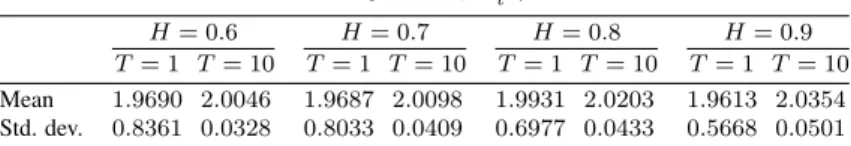
Tables 1 and 2 contain the results of numerical simulations for model (23) withα = 1
andα= 2, respectively. ForT = 1andT = 10and various values ofH, we findhT
directly by (24). Forθ= 2, we simulate 1000 realizations of the process for eachH and compute the values ofθˆT by (13). The means and standard deviations of these estimates
are reported. We see that these simulation studies confirm the consistency ofθˆT. The
results are quite similar for different values ofH. Moreover, the increase ofαincreases the rate of convergence.
Table 1.Xt=θt2+BHt ,θ= 2. H= 0.6 H= 0.7 H= 0.8 H= 0.9 T = 1 T = 10 T = 1 T = 10 T= 1 T = 10 T= 1 T= 10 Mean 1.9690 2.0046 1.9687 2.0098 1.9931 2.0203 1.9613 2.0354 Std. dev. 0.8361 0.0328 0.8033 0.0409 0.6977 0.0433 0.5668 0.0501 Table 2.Xt=θt3+BHt ,θ= 2. H= 0.6 H= 0.7 H= 0.8 H= 0.9 T = 1 T = 10 T = 1 T = 10 T= 1 T = 10 T= 1 T= 10 Mean 1.9820 2.0001 1.9847 2.0002 1.9512 1.9994 1.9827 1.9964 Std. dev. 0.7009 0.0027 0.6046 0.0032 0.5153 0.0033 0.3625 0.0033
Acknowledgment. The authors are grateful to Alexei Konstantinov for advice on the short proof of Lemma A.1. We would like to thank three anonymous referees for their useful comments and suggesting a number of improvements.
Appendix
Lemma A.1. Iff ∈L2[0, T], then
lim n→∞ n X k=1 kT /n Z (k−1)T /n f(t)−n T kT /n Z (k−1)T /n f(s) ds !2 dt= 0. (A.1)
Proof. The lemma follows from the criterion of strong convergence of linear operators, since (A.1) holds true if the functionf(x)is continuous, the continuous functions make a dense set inL2[0, T], and the sequence of linear operators
An(f) =f − n X k=1 n T kT /n Z (k−1)T /n f(s) ds1((k−1)T /N, kT /N], f ∈L2[0, T],
Lemma A.2. Iff ∈L2[0, T],g∈L2[0, T], then one can choose a sequence of piecewise
constant functions {fn(s), n > n0} (the function fn(s) is constant on the intervals
((k−1)T /n, kT /n))such thatlimn→∞R
T
0 (f(s)−fn(s))
2ds= 0, and, for sufficiently
largen,R0Tfn(t)g(t) dt=
RT
0 f(t)g(t) dt.
Proof. Ifg(t) = 0almost everywhere on[0, T], then the statement of the lemma follows from Lemma A.1. In what follows, we assume thatg(t)is not zero everywhere. This is equivalent toR0T|g(s)|ds >0. Put sn(t) = sign kT /n Z (k−1)T /n g(s) ds ! , (k−1)T n < t < kT n ; Vn = T Z 0 sn(t)g(t) dt= n X k=1 kT /n Z (k−1)T /n g(s) ds. Then lim n→∞Vn= Var[0,T] t Z 0 g(s) ds= T Z 0 g(s)ds >0. (A.2)
In particular,Vn>0for sufficiently largen. Put
φn(t) = n T kT /n Z (k−1)T /n f(s) ds, (k−1)T n < t < kT n ; fn(t) =φn(t) + RT 0 (f(s)−φn(s))g(s) ds Vn sn(t). (A.3)
Thenφn →f inL2[0, T]. Therefore, the numerator in (A.3) tends to0. It follows from
the uniform boundedness ofsn(t)and (A.2) thatfn→f inL2[0, T]. Moreover,
T Z 0 fn(t)g(t) dt = T Z 0 φn(t)g(t) dt+ RT 0 (f(s)−φn(s))g(s) ds Vn T Z 0 sn(t)g(t) dt = T Z 0 φn(t)g(t) dt+ T Z 0 f(s)−φn(s)g(s) ds= T Z 0 f(t)g(t) dt
for allnsuch thatVn >0.
Lemma A.3. Let M be a positively definiten×n-matrix, aand b ben-dimensional vectors. Thena>M ab>M−1b
Proof. The statement of the lemma holds ifb = 0. Otherwise,M−1 is also positively definite, therefore,b>M−1b >0. Then
06 a− (a >b) b>M−1bM −1b > M a− (a >b) b>M−1bM −1b =a>M a−2 (a >b) b>M−1bb >M−1M a+ (a>b)2 (b>M−1b)2b >M−1M M−1b =a>M a− (a >b)2 b>M−1b.
Lemma A.4. Let0< p <1andb >0.
(i) Ify∈L1[0, b]is a solution to integral equation
b
Z
0
y(s) ds
|t−s|p =f(t) (A.4)
for almost allt∈(0, b), theny(x)satisfies
y(x) =Γ(p) cos πp 2 πx(1−p)/2 D (1−p)/2 b− x1−pD(10+−p)/2 f(x) x(1−p)/2 (A.5)
almost everywhere on[0, b], whereDα
a+andDbα−are fractional derivatives, Dα a+f(x) = 1 Γ(1−α) d dx x Z a f(t) (x−t)αdt ! , Dα b−f(x) = −1 Γ(1−α) d dx b Z x f(t) (t−x)αdt ! .
(ii) Ify1 ∈ L1[0, b]andy2 ∈ L1[0, b]are two solutions to integral equation(A.4),
theny1(x) =y2(x)almost everywhere on[0, b].
(iii) If y ∈ L1[0, b] satisfies (A.5) almost everywhere on [0, b] and the fractional
derivatives are solutions to respective Abel integral equations, that is,
1 Γ(1−2p) t Z 0 D(10+−p)/2(f(x)x(p−1)/2) (t−x)(p+1)/2 dx= f(t) t(1−p)/2 (A.6)
for almost allt∈(0, b)and
1 Γ(1−2p) b Z x πy(s)s(1−p)/2 Γ(p) cosπp2 ds (s−x)(p+1)/2 =x 1−pD(1−p)/2 0+ f(x) x(1−p)/2 (A.7)
Sketch of proof. The integral equation is solved in [6, 11]. In [6, Sect. 2.3], the equation is rewritten as t(1−p)/2 B(p,1−2p) t Z 0 1 (t−τ)(p+1)/2τ1−p b Z τ s(1−p)/2y(s) ds (s−τ)(p+1)/2 dτ=f(t).
For the new equation, the statement of the theorem can readily be obtained.
Lemma A.5. Let1/2< p <1and0< ξ < b. Then the integral equation
b
Z
0
y(s) ds
|s−t|p =1[ξ,b](t) for almost allt∈[0, b] (A.8) has a unique solutiony∈L2[0, b].
Proof. By Lemma A.4, if the solution to (A.8) exists withinL1[0, b], it is equal to
y(x) = Γ(p) cos πp 2 πΓ(p+12 )x(1−p)/2D (1−p)/2 b− x 1−p d dx " x Z 0 1[ξ,b](s) ds s(1−p)/2(x−s)(1−p)/2 #! .
Note that the function
x Z 0 1[ξ,b](s) ds s(1−p)/2(x−s)(1−p)/2 = ( 0 for06x6ξ, xpB(1−ξx;p+12 ,p+12 ) forξ6x6b (A.9)
is absolutely continuous on [0, b] and is equal to 0 at the neighbourhood of 0 (here
B(x;α, β) = Rx
0 t
α−1(1−t)β−1dt is the incomplete beta function). Then, by [17,
Thm. 2.1], its derivative is a solution to Abel integral equation
1 Γ(1−2p) x Z 0 1 Γ(p+12 ) d dt t Z 0 1[ξ,b](s) ds s(1−p)/2(t−s)(1−p)/2 ! dt (x−t)(p+1)/2 = 1[ξ,b](x) x(1−p)/2.
Thus, condition (A.6) holds true forf(x) =1[ξ,b](x).
The derivative of the right-hand side of (A.9) forx>ξis equal to
d dx x Z ξ ds s(1−p)/2(x−s)(1−p)/2 ! = p x1−pB 1−ξ x; p+1 2 , p+1 2 + ξ (p+1)/2 x(x−ξ)(1−p)/2. Thus, y(x) = Γ(p) cos πp 2 πΓ(p+12 )x(1−p)/2 D (1−p)/2 b− G1(x) +D (1−p)/2 b− G2(x) (A.10)
with G1(x) = pB(1 −ξ/x; (p+ 1)/2,(p+ 1)/2)1(ξ,+∞)(x), G2(x) = ξ(p+1)/2/
(xp(x−ξ)(1−p)/2)1(ξ,+∞)(x).
The function G1(x) is continuous, therefore G1 ∈ L2[0, T]. Also, it is piecewise
differentiable and Hölder with exponent(1 +p)/2. Consequently, its fractional derivative Db(1−−p)/2G1is bounded on any interval[0, b1],0< b1< b, see [17, Thm. 13.6]. It makes
a solution to Abel integral equation: Ib(1−−p)/2Db(1−−p)/2G1 = G1almost everywhere on
(0, b). At the neighbourhood ofb, it has the asymptotic behaviour: Db(1−−p)/2G1(x) ∼
G1(b)/(Γ((p+ 1)/2)(b−x)(1−p)/2),x→b−. Thus,D (1−p)/2
b− G1∈L2[0, b].
The function G2(x) is piecewise continuous, unbounded asx → ξ+, and G2 ∈
L2[0, b]. In order to prove thatD (1−p)/2
b− G2∈L2[0, T], we use Theorem 13.2 from [17],
according to which,Ib(1−−p)/2Db(1−−p)/2G2 =G2andD (1−p)/2
b− G2 ∈L2[0, b]if and only
if two conditions hold: (i)G2 ∈L2[0, b]; and (ii)ψ converges inL2[0, b]as →0+,
where ψ(x) = Rb x+ G2(t)−G2(x) (t−x)(3−p)/2 dt, 06x6b−, Rb x+ −G2(x) dt (t−x)(3−p)/2 = −2G2(x) 1−p ( 1 (1−p)/2 − 1 (b−x)(1−p)/2), b−6x < b,
forb−6x < b. Condition (i) holds true. Condition (ii) is an immediate consequence of the following assertions:
• The integrand, which equals either(G2(t)−G2(x))(t−x)(p−3)/2ifx+6t6b
or−G2(t)(t−x)(p−3)/2ifb6t6x+,t > x, is positive or zero if06x6ξ
and negative ifξ < x < b. Therefore, for fixedx,ψ(x)is monotonous in.
• At=b, ψb(x) = ( 0, 06x6ξ, 2 1−p ξ(p+1)/2 xp(x−ξ)(1−p)/2( 1 (b−x)(1−p)/2− 1 b(1−p)/2), ξ < x < b, belongs toL2[0, T]. • At= 0, ψ0(x) = b Z x G2(t)−G2(x) (t−x)(3−p)/2 dt, and ψ0(x) < const |x−ξ|1−p with const =ξ(1−p)/21 +p 1−p ∞ Z 0 du u(1−p)/2(1 +u)(3−p)/2 < ξ(1−p)/2(3−p) (1−p)2 . Therefore,ψ0∈L2[0, b].
• lim→0+ψ(x) = ψ0(x) for all x, 0 6 x < b, because the Lebesgue integral
is continuous-on-the-right with respect to the lower limit. The limit is finite at the points where ψ0(x) is finite, i.e., almost everywhere on (0, b); however
lim→0+ψ(ξ) = +∞=ψ0(ξ).
Thus,D(1b−−p)/2G2∈L2[0, b]. Moreover, forx < ξ, the function
D(1b−−p)/2G2(x) = 1 Γ(p−21) b Z ξ G2(t) dt (t−x)(3−p)/2
is bounded in the neighbourhood of0. Since the function Db(1−−p)/2G1(x) +D
(1−p)/2
b− G2(x)is square integrable on(0, b)
and bounded in the neighbourhood of0, multiplying it byx(p−1)/2does not drive it out
ofL2[0, b]. Thus,y∈L2[0, b], see (A.10). From (A.10) and equalities
Ib(1−−p)/2Db(1−−p)/2G1=G1 and I (1−p)/2 b− D (1−p)/2 b− G2=G2 it follows that Ib(1−−p)/2 πΓ(p)y(x)x(1−p)/2 Γ(p) cosπp2 =G1(x) +G2(x) =x1−pD (1−p)/2 0+ 1 [ξ,b](x) x(1−p)/2 .
Condition (A.7) holds true. By statement (iii) of Lemma A.4,y(x)is indeed a solution to integral equation (A.8). Uniqueness of the solution to (A.8) follows from statement (ii) of Lemma A.4 and from the fact thatL2[0, b]⊂L1[0, b].
References
1. T.V. Anderson,An Introduction to Multivariate Statistical Analysis, Wiley, Hoboken NJ, 2003. 2. J. Berger, R. Wolpert, Estimating the mean function of a Gaussian process and the Stein effect,
J. Multivariate Anal.,13(3):401–424, 1983.
3. K. Bertin, S. Torres, C. A. Tudor, Maximum-likelihood estimators and random walks in long memory models,Statistics,45(4):361–374, 2011.
4. T. Bojdecki, L.G. Gorostiza, A. Talarczyk, Sub-fractional Brownian motion and its relation to occupation times,Stat. Probab. Lett.,69(4):405–419, 2004.
5. V. Buldygin,Convergence of Random Elements in Topological Spaces, Naukova Dumka, Kyiv, 1980 (in Russian).
6. C. Cai, P. Chigansky, M. Kleptsyna, The maximum likelihood drift estimator for mixed fractional Brownian motion, 1st version, arXiv:1208.6253v1.
7. C. Cai, P. Chigansky, M. Kleptsyna, Mixed Gaussian processes: A filtering approach, Ann. Probab.,44(4):3032–3075, 2016.
8. K. Es-Sebaiy, I. Ouassou, Y. Ouknine, Estimation of the drift of fractional Brownian motion,
9. Y. Hu, D. Nualart, W. Xiao, W. Zhang, Exact maximum likelihood estimator for drift fractional Brownian motion at discrete observation,Acta Math. Sci., Ser. B, Engl. Ed.,31(5):1851–1859, 2011.
10. I.A. Ibragimov, Y.A. Rozanov, Gaussian Random Processes, Appl. Math. (N. Y.), Vol. 9, Springer, New York, Berlin, 1978.
11. A. Le Breton, Filtering and parameter estimation in a simple linear system driven by a fractional Brownian motion,Stat. Probab. Lett.,38(3):263–274, 1998.
12. Yu. Mishura, Maximum likelihood drift estimation for the mixing of two fractional Brownian motions, inStochastic and Infinite Dimensional Analysis, Birkhäuser, Basel, 2016, pp. 263– 280.
13. Yu. Mishura, K. Ralchenko, S. Shklyar, Maximum likelihood drift estimation for Gaussian process with stationary increments,Austrian J. Stat.,46(3–4):67–78, 2017.
14. Yu. Mishura, I. Voronov, Construction of maximum likelihood estimator in the mixed fractional-fractional Brownian motion model with double long-range dependence,Mod. Stoch., Theory Appl.,2(2):147–164, 2015.
15. I. Norros, E. Valkeila, J. Virtamo, An elementary approach to a Girsanov formula and other analytical results on fractional Brownian motions,Bernoulli,5(4):571–587, 1999.
16. N. Privault, A. Réveillac, Stein estimation for the drift of Gaussian processes using the Malliavin calculus,Ann. Stat.,36(5):2531–2550, 2008.
17. S. Samko, A. Kilbas, O. Marichev,Fractional Integrals and Derivatives, Gordon and Breach, Yverdon, 1993.
18. P.A. Samuelson, Rational theory of warrant pricing,Ind. Manag. Rev.,6(2):13–32, 1965. 19. G. Shen, L. Yan, Estimators for the drift of subfractional Brownian motion, Commun. Stat.,
Theory Methods,43(8):1601–1612, 2014.
20. C. Tudor, Some properties of the sub-fractional Brownian motion,Stochastics,79(5):431–448, 2007.