Unsupervised feature selection by means of external validity indices

Validity Indices

Javier Béjar

Departament de Llenguatges i Sistemes Informàtics

Universitat Politècnica de Catalunya

[email protected]

Feature selection for unsupervised data is a difficult task because a reference partition is not available to evaluate the relevance of the features. Recently, different proposals of methods for consensus clustering have used external validity indices to assess the agreement among partitions obtained by clustering algorithms with different parameter values. Theses indices are independent of the characteristics of the attributes describing the data, the way the partitions are represented or the shape of the clusters. This independence allows to use these measures to assess the similarity of partitions with different subsets of attributes.

As for supervised feature selection, the goal of unsupervised feature selection is to maintain the same patterns of the original data with less information. The hypothesis of this paper is that the clustering of the dataset with all the attributes, even when its quality is not perfect, can be used as the basis of the heuristic exploration the space of subsets of features. The proposal is to use external validation indices as the specific measure used to assess well this information is preserved by a subset of the original attributes.

Different external validation indices have been proposed in the literature. This paper will present experi-ments using the adjusted Rand, Jaccard and Folkes&Mallow indices. Artificially generated datasets will be used to test the methodology with different experimental conditions such as the number of clusters, cluster spatial separanton and the ratio of irrelevant features. The methodology will also be applied to real datasets chosen from the UCI machine learning datasets repository.

1 Introduction

To reduce the dimensionality of a dataset is an important task in machine learning and data mining. It has two advantages, it reduces the computational cost of processing the dataset and it improves the interpretability of the results. Feature selection is a method for dimensionality reduction that eliminates from a dataset all the attributes that are not relevant to the task to be solved. The main advantage of this methods in front of others, like feature extraction, is that the original attributes are preserved and the obtained model is easier to interpret.

Most of the research on feature selection is related to supervised tasks [13]. More recently methods for unsupervised tasks have been appearing in the literature ([14], [16], [5]). Most of these methods are based on characteristics of the features or characteristics of the model obtained by the clustering algorithm. Our proposal is to use measures that use only external properties of the partitions, so they can be applied independently of the characteristics of the features of the dataset or the representation of the partition.

The next section will review the recent literature on unsupervised feature selection. Section 3 will show the different external validity indices used in the experiments. Section 4 will explain the algorithm used to explore the attribute space to perform the attribute selection. Section 5 will show experiments with different artificial and real datasets and the results obtained. Section 6 will summarize the conclusions and future work.

2 Related work 2

2 Related work

The problem of feature selection can be defined as follows:

Having a set of features D and a dataset X that contains N instantiations of the set of features, obtain a subset of featuresS (S⊆D) that maintains the relevant information of the dataset for the learning goal.

For supervised features selection the learning goal is defined by a set of labelsthat classify all the instances in the dataset in groups. For unsupervised feature selection the learning goal has to be related to an hypothetical inherent structure of the data.

The classification of methods for feature selection has been established in the supervised feature selection literature, and can be roughly applied also to unsupervised feature selection. The methods can be summarized as:

• The filter approach: Features are assessed individually using the task goal and a relevance value is computed that is used to order the features

• The wrapper approach: Features are assessed in subsets, an algorithm that performs the learning task is used for this assessment.

• The embedded approach: The selection of the most relevant features is an integrated part of the learning task.

Usually feature selection involves two elements, a criteria to be used to measure the relevance of a feature or a subset of features, and a search strategy.

In the filter approach the most important element is the relevance criteria. In supervised feature selection the relevance criteria is related to the labels of the example in the dataset. In unsupervised feature selection there is a more wide diversity of criteria. As the labels are unknown the criteria has to rely on general characteristics of the data such as global or local structure preservation. The search strategy is the criteria to be used to determine the cutting point in the ordered list of features.

There are several examples of this methods in the literature. In [4] is presented a measure based on entropy that evaluates if a dataset presents a structure according with the distribution of the examples. This measure allows to compare different subsets of attributes without clustering the data and to obtain a rank of the attributes. In [9] consensus clustering is used based on clusters obtained by selecting random subsets of features. The consensus allows to compute a ranking of the features based on the correlation of the features within the clusterings. In [22] a correlation measure is used, iteratively features are ranked and selected assuming that the dataset can be obtained by a linear combination of the features. Some other methods rank features using measures that determine how well the local structure is preserved like the Laplacian score [8, 18] or measures related to spectral clustering [23, 25].

In the wrapper approach the search strategy is the most important element. The problem is to be able to select the best subset of features from an exponential number of combinations. This means that an efficient search strategy is crucial. Supervised feature selection uses as a criteria a supervised learning algorithm and performs a search to obtain the minimum subset with the best accuracy. Unsupervised feature selection has to use a clustering algorithm as a method to discover the structure of the data. The search is performed to look for the set of features that preserves the apparent structure of the data obtained by the clustering algorithm.

Some examples of this approach include selection strategies based on internal validation measures the like silhouette index and forward selection as search algorithm [11] or consensus clustering based on random subspaces as measure of feature relevance and genetic algorithms as search strategy [10]. Several approaches propose to extend the problem as a multicriteria optimization problem to solve simultaneously the feature selection problem and the selection of the number of cluster. In these methods, different variations of genetic algorithms are used as search methodology combined with different internal validation measures like the Davis-Bouldin criteria [12, 15, 17, 2].

In the embedded approach a model is assumed in the data. This model usually includes two goals, to determine the number of clusters that describes the structure of the data, and to determine the set of features that better describes the clusters. These two goals are tightly related, so the method is to obtain both simultaneously.

This approach assumes a model based on the mixture of probability distributions, usually gaus-sians, and extends the model by introducing as parameters of the distribution the selection of the features using weighting schemes (binary or continuous) and the number of components of the mix-ture. The algorithm used to fit the model is usually the Expectation-Maximization algorithm combined with a model selection strategy based on measures of feature salience, model complexity or cluster quality [14, 5, 3, 20, 24]

3 External validity indices

Cluster validity indices [7] are used to assess the validity of the partitions obtained by a clustering algorithm by comparing its characteristics to a reference or ideal partition. These indices give a relative or absolute value to the similarity among different partitions of the same data.

These indices can be classified in external criteria, internal criteria and relative criteria. The first ones assume that the evaluation of a partition is based on a pre-specified structure that reflects the natural structure of the dataset. For the second ones, the evaluation is performed in terms of quantities obtained from the values of the attributes that describe the clusters, that measure how separated and compact are. The last ones assume that the evaluation is performed comparing the partition to other partitions obtained using different parameters of the clustering algorithm or from other clustering algorithms. In our approach, we are interested on the first kind of validity indices.

External validity indices allow to compare different partitions independently of the type of the attributes used to describe the dataset, the distance function used to measure the similarity of the examples or the model used by the clustering algorithm. In order to do that, only the cluster co-association of the examples between pairs of is used.

The main idea of these indices is that when two examples belong to a natural cluster in the data, they usually appear in the same group when different partitions are obtained. This means that two partitions that maintain these co-association are more similar and represent a similar structure for the dataset.

In order to compute these indices the coincidence of each pair of examples in the groups of two clusterings has to be counted, there are four possible cases:

• The two examples belong to the same class in both partitions (a)

• The two examples belong to the same class inC, but not inP (b)

• The two examples belong to the same class inP, but not inC (c)

• The two examples belong to different classes in both partitions (d)

From this values different similarity indices can be defined for comparing two partitions:

• Adjusted Rand statistic:

AR= a− (a+c)(a+b) a+b+c+d (a+c)+(a+b) 2 − (a+c)(b+c) a+b+c+d • Jaccard Coefficient: J = a (a+b+c)

4 Exploration of the attribute space 4

• Folkes and Mallow index:

F M =

r _a

a+b·

a

a+c

One of the interesting properties of all this three indices is that they are in the range [0,1] making more easier to compare their results.

4 Exploration of the attribute space

Being our task unsupervised, there is no ground truth we can use for comparison purposes. To solve this problem, we are going to choose the partition obtained with all the attributes. This partition will be called the reference partition. The actual labels of the examples are not needed, if we can define some similarity/quality measure with this partition. The search for a clustering with a reduced number of attributes will be guided by this similarity measure as heuristic.

The task will be to find the subset of attributes that obtains the partition more similar to the reference partition. We will use a wrapper approach. As this task would need to explore all possible subsets we are going to use a best first strategy to reduce the computational cost.

This exploration of the feature space is going to be performed using theforward selection strategy. This strategy is also used in wrapper based methods in supervised feature selection [13]. In this case we are going to substitute the supervised algorithm used for the evaluation of attribute subsets by a validity index. This validity index will compute the similarity between the partition obtained with the subset of features and the reference partition.

The forward selection strategy begins with an empty set of attributes and the reference partition. Each step evaluates all partitions that can be obtained by adding one new attribute from the attribute list. If the subset more similar to the reference partition increases the similarity with respect to the one obtained in the previous previous step, that subset is retained, growing the selected list of attributes. The process is iterated using this new subset of attributes. The exploration is stopped when no more attributes can be added obtaining an increase of similarity larger than a threshold α. The detailed algorithm is presented as algorithm 1.

The parameter α will be in the range [0,1] accordingly with the values of the external index used to measure similarity. There is not a priori good value for this parameter. If the value is closer to 0 less increase of similarity respect to the previous iteration will be needed to include new attributes. If the value is too high the algorithm will stop with only a few attributes selected. As similarity will increase monotonically with the number of attributes a criteria to decide its value is to consider what is the minimum percentage of similarity a new attribute has to add to be considered relevant.

5 Experiments

For the experiments, different datasets will be used. First, synthetic datasets generated with different characteristics will be used, so the feature selection methodology can be tested in a wide range of types of datasets. Specifically, it will be tested the performance with different number of partitions, different spatial separation among the clusters, different number of relevant attributes and different ratio of irrelevant attributes.

The methodology will be also tested with datasets from the UCI machine learning repository [6]. The cluster algorithm used as wrapper algorithm will be k-means using the actual number of clusters as the value of k. To reduce the sensitivity of this algorithm to initialization the k-means++ ([1]) algorithm is used.

5.1 Synthetic datasets

The first set of experiments has been performed using synthetic datasets with different number of clus-ters and irrelevant attributes. The datasets have been generated using the R packageclusterGeneration

Algorithm 1 Greedy forward selection Procedure: Greedy_Forward_Selection(DataSet,AttributeSet) ReferenceClustering= Cluster(DataSet,AttributeSet) QualityIncrease=true BestSimilarity=0 BestClustering=∅ CurrentAttributeSet=∅ while QualityIncrease do BestNewSimilarity= 0 BestAttibute= ∅ BesNewClustering=∅

for attribute ∈ AttributeSet do

IAtrributeSet= CurrentAttributeSet + attibute CurrenClustering= Cluster(DataSet,IAttributeSet)

CurrentSimilarity= ValidityIndex(ReferenceClustering, CurrentClustering)

if CurrentSimilarity>BestNewSimilarity then

BestNewSimilarity= CurrentSimilarity BestNewAttibute= attribute BestNewClustering= CurrentClustering end end if BestNewSimilarity-BestSimilarity > α then

AttributeSet= AttributeSet - BestNewAttibute

CurrentAttributeSet = CurrentAttributeSet + BestNewAttibute BestClustering= BestNewClustering BestSimilarity= BestNewSimilarity else QualityIncrease = false end end return CurrentAttributeSet

The data generated corresponds to sets of ellipsoidal clusters described by attributes modeled using gaussian distributions. These attributes can be divided into relevant and irrelevant attributes. The relevant attributes are the same for all clusters and are generated independently using random orthonormal matrices. Also random rotations are applied to the generated clusters. This means that each cluster has ellipsoidal shape with axis oriented in arbitrary directions. The irrelevant attributes are randomly generated using gaussian distributions with a variance similar to the sample variance of the relevant attributes.

The methodology for generating the data allows to control the minimum degree of separation for a cluster respect to the other clusters. This makes possible to generate datasets with different degrees of separation, from highly overlapped to well separated clusters. Figure 1 shows two datasets using 3 relevant attributes with 3 clusters and different separation.

In the experiments we will vary the number of clusters, the number of attributes, the ratio between the number of irrelevant and irrelevant attributes and the degree of separation between pairs of clusters. Specifically, the datasets have been generated for 3, 5 and 10 clusters with around 100 examples per cluster. The datasets with 3 and 5 clusters have been generated using 5 and 10 relevant attributes, and the datasets with 10 clusters have been generated with 10 and 20 relevant attributes. For each dataset, a set of irrelevant attributes has been added in the same amount, twice and four times the number of relevant attributes. Clusters are also generated with different degrees of separation, using 0, 0.01 and 0.1 as the values of the parameter that controls the degree of separation in the dataset

5 Experiments 6 Sep=0 ● ● ● ● ● ● ● ● ● ● ● ● ● ● ● ● ● ● ● ● ● ● ● ● ● ● ● ● ● ● ● ● ● ● ● ● ● ● ● ● ● ● ● ● ● ● ● ● ● ● ● ● ● ● ● ● ● ● ● ● ● ● ● ● ● ● ● ● ● ● ● ● ● ● ● ● ● ● ● ● ● ● ● ● ● ● ● ● ● ● ● ● ● ● ● ● ● ● ● ● ● ●● ● ● ● ● ● ● ● ● ● ● ● ● ● ● ● ● ● ● ● ● ● ● ● ● ● ● ● ● ● ● ● ● ● ● ● ● ●● ● ● ● ● ● ● ● ● ● ● ● ● ● ● ● ● ● ● ● ● ● ● ● ● ● ● ● ● ● ● ● ● ● ● ● ● ● ● ● ● ● ● ● ● ● ● ● ● ● ● ● ● ● ● ● ● ● ● ● ● ● ●● ● ● ● ● ● ● ● ● ● ● ● ● ● ● ● ● ● ● ● ● ● ● ● ● ● ● ● ● ● ● ● ● ● ● ● ● ● ● ● ● ● ● ● ● ● ● ● ● ● ● ● ● ● ● ● ● ● ● ● ● ● ● ● ● ● ● ● ● ● ● ● ● ● ● ● ● ● ● ● ● ● ● ● ● ● ● ● ● ● ● ● ● ● ● ● ● ● ●● ● ● ● ● ● ● ● ● ● ● ● ● ● ● ● ● ● ● ● ● ● ● ● ● ● ● ● ● ● ● ● ● ● ● ● ● ● ● ● ● ● ● ● ● ● ● ● ● ● ● ● ● ● ● ● ● ● NN9 NN10 NN3 Sep=0.1 ● ● ● ● ● ● ● ● ● ● ● ● ● ● ● ● ● ● ● ● ● ● ● ● ● ● ● ● ● ● ● ● ● ● ● ● ● ● ● ● ● ● ● ● ● ● ● ● ● ● ● ● ● ● ● ● ● ● ● ●● ● ● ● ● ● ● ● ● ● ● ● ● ● ● ● ● ● ● ● ● ● ● ● ● ● ● ● ● ● ● ● ● ● ● ● ● ● ● ● ● ● ● ● ● ● ● ● ● ● ● ● ● ● ● ● ● ● ● ● ● ● ● ● ● ● ● ● ● ● ● ● ● ● ● ● ● ● ● ● ● ● ● ● ● ● ● ● ● ● ● ● ● ● ● ● ● ● ● ● ● ● ● ● ● ● ● ● ● ● ● ● ● ● ● ● ● ● ● ● ● ● ● ● ● ● ● ● ● ● ● ● ● ● ● ● ● ● ● ● ● ● ● ● ● ● ● ● ● ● ● ● ● ● ● ● ● ● ● ● ● ● ● ● ● ● ● ● ● ● ● ● ● ● ● ●● ● ● ● ● ● ● ● ● ● ● ● ● ● ● ● ● ● ● ● ● ● ● ● ● ● ● ● ● ● ● ● ● ● ● ● ● ● ● ● ● ● ● ● ● ● ● ● ● ● ● ● ● ● ● ● ● ● ● ● ● ● ● ● ● ● ● ● ● ● ● ● ● ● ● ● ● ● ● ● ● ● ● ● ● ● ● ● ● ● ● ● ● ● ● ● ● ● ● ● ● ● ● ● ● ● ● ● ● ● ● ● ● ● ● ● ● ● ● NN7 NN3 NN6

Fig. 1: Synthetic datasets with 3 clusters and separation 0 and 0.1

generation program.

The number of relevant attributes used for generating each dataset is not always the exact number of attributes needed for uncovering the clusters. This number actually depends on the degree of separation among the clusters. To be able to perform fair comparisons the actual list of the relevant attributes for each dataset has been computed using wrapper methodology by performing forward selection using a naive bayes classifier. The mean accuracy of the naive bayes classifiers for the datasets with only the selected attributes is 0.93 with a standard deviation of 0.03.

As performance measures three criteria will be used:

• The similarities to the true labels of the reference partition and the partition obtained using the relevant attributes.

• The number of attributes used to generate the clusters compared to the number attributes after the unsupervised selection.

• The intersection between the list of relevant attributes selected by the unsupervised algorithm and the list of relevant attributes selected by the supervised algorithm.

5.1.1 Comparison of the measures

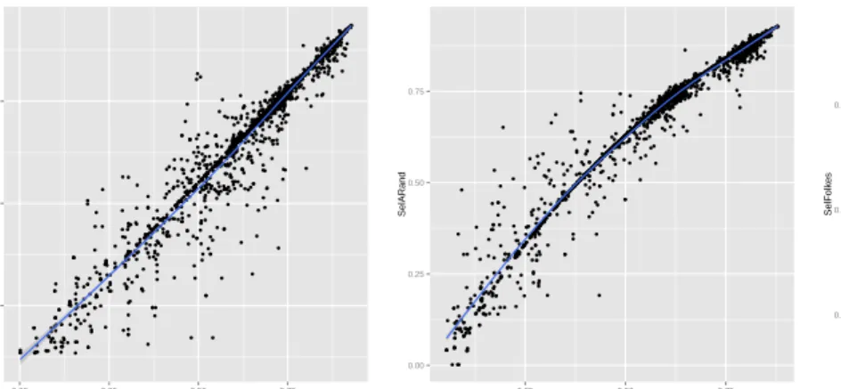
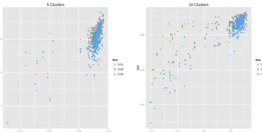
We will first compare the behavior of the three indices in the experiments. All three use the same information for computing the similarity of partitions, so they are expected to yield similar results. In figure 2 the values of all three measures are plotted against each other for all the experiments with 10 clusters. As it can be seen, the behavior of the Adjusted Rand and the Folkes & Mallow indices are clearly linearly correlated. The Jaccard index shows a slightly nonlinear correlation with the other two indices. This means that the first two indices tend to move their values to the extremes of the interval.

From the distribution of the measures for all the experiments (see figure 3), it can be seen that the distributions of the indices are very close. The Adjusted Rand index is closer to the Jaccard index when there are less clusters and to the Folkes & Mallow index when the number of clusters is larger. A Pearson correlation test over the variables for each different number of clusters shows that the correlation among the three indices is around 0.97 with 99% of confidence. Due to this high correlation among the indices and because the Adjusted Rand index is the most well-known and studied [21], only its value will be shown for the rest of the experiments.

● ● ● ● ●● ● ●●● ●● ● ●● ● ● ● ●● ● ● ● ● ● ● ● ● ● ● ● ●● ● ● ● ● ● ● ● ● ●● ● ● ● ● ● ●●● ● ● ● ● ● ● ● ● ● ● ● ● ●● ● ● ● ● ● ● ● ● ● ● ● ● ● ●●● ● ● ● ● ● ● ● ● ● ● ● ● ● ● ● ● ● ● ● ●● ●● ● ● ● ●● ● ● ● ● ●● ● ● ● ● ●● ● ● ● ● ● ● ● ● ● ●● ●● ● ● ● ●● ● ● ● ●● ● ● ● ● ● ● ● ● ● ● ● ●● ● ●●● ● ● ●●● ● ● ● ●● ● ●● ● ● ● ● ● ● ● ● ● ● ● ● ● ● ● ● ● ●● ● ● ●● ● ●●● ● ● ● ● ● ● ● ● ● ● ● ● ● ● ● ● ● ● ● ● ● ● ●●● ● ● ● ● ● ● ● ● ● ● ● ● ● ● ● ● ● ● ● ● ● ● ●● ● ● ●● ● ● ● ● ● ● ● ● ● ●●● ● ● ●●● ● ● ● ● ● ● ● ● ● ●● ●● ● ●●● ● ● ● ● ● ● ● ●● ● ● ● ● ● ● ● ● ●● ● ●●● ● ● ●●● ● ● ● ●● ● ●● ● ● ● ● ● ● ● ●● ● ● ● ● ● ● ● ● ●● ● ● ● ● ● ●● ● ● ● ● ● ● ● ●●● ● ● ● ●● ● ● ● ● ● ● ● ●●●● ● ● ● ● ● ● ● ● ● ● ● ● ● ● ● ● ● ● ● ● ● ● ●● ● ● ●● ● ● ● ● ● ● ●● ● ●●● ● ● ●●● ● ● ● ● ● ● ● ● ● ●● ●● ● ● ● ● ● ● ● ● ● ● ● ● ● ● ● ● ● ● ● ● ● ● ● ● ● ● ● ● ●● ● ● ● ● ● ● ● ●●● ● ● ● ● ● ● ● ● ● ● ● ● ● ● ●●● ● ● ● ● ● ● ● ● ● ●● ● ● ● ● ● ● ● ● ● ● ● ● ● ● ● ● ●● ● ● ● ● ● ● ● ● ●● ● ● ● ● ● ●● ● ●●● ● ● ● ● ● ● ● ● ● ● ●●● ● ● ● ●● ● ● ● ● ●● ● ● ● ● ● ● ● ● ● ● ● ●● ● ● ● ● ● ●● ● ● ● ● ● ● ● ● ● ● ● ● ● ●● ● ● ● ● ● ● ● ● ● ● ● ● ●● ● ● ● ● ● ● ● ● ● ● ● ● ● ● ●● ● ● ● ● ● ● ● ● ●● ● ● ● ● ● ● ● ● ●●● ● ● ● ● ● ● ● ● ●● ● ● ● ●● ● ● ● ● ● ● ● ● ● ● ● ● ● ● ● ● ● ● ●● ● ● ●●● ● ● ● ● ● ● ● ● ● ● ●● ● ● ● ● ● ● ● ●●●●●●●● ● ● ● ● ● ● ● ● ● ● ● ● ● ● ● ● ● ● ● ● ● ● ● ● ●●● ● ● ● ●● ● ● ● ● ● ● ● ● ● ● ●●●●● ● ● ● ● ● ● ● ● ● ●● ● ● ●● ● ● ● ● ● ● ● ● ●● ● ● ● ● ● ● ● ● ● ●●● ● ● ● ● ● ● ● ●● ● ● ● ● ● ●●● ● ● ● ● ● ● ● ● ● ● ● ● ● ● ● ●● ● ● ●●● ● ● ● ● ● ● ● ● ● ● ● ● ● ● ● ● ● ● ● ●●● ● ●●●●●● ● ● ● ● ● ● ● ● ● ● ● ● ● ● ● ● ● ●● ● ● ● ●●● ● ● ● ●● ● ● ● ● ● ● ● ● ● ● ● ● ● ● ●● ● ● ● ● ● ● ● ● ● ● ● ● ● ● ● ● ● ● ● ● ● ● ● ● ● ● ● ● ● ● ● ● ● ● ● ● ● ● ● ● ● ● ● ● ● ● ● ● ● ● ● ● ● ● ● ● ● ● ● ● ● ● ● ● ● ● ● ● ● ● ● ● ● ● ● ● ● ● ● ● ● ● ● ● ● ● ● ●● ● ● ● ● ● ● ●●● ● ●● ● ●●● ● ●● ●● ● ●● ● ●● ● ● ●● ● ● ● ●● ● ● ●● ● ● ● ● ● ● ● ● ● ● ● ● ● ● ● ● ● ● ● ●● ● ● ● ● ● ● ● ● ● ● ● ● ● ● ● ● ● ● ● ● ● ● ● ● ● ● ● ● ● ● ● ● ● ● ● ● ● ● ● ● ● ● ● ● ● ● ● ● ● ● ● ● ● ● ● ● ● ● ● ● ● ● ● ● ● ● ● ● ● ● ●● ● ● ● ● ● ● ● ● ● ● ● ● ● ● ● ●● ● ● ● ● ● ● ● ● ● ●●● ● ●●● ● ●● ●● ● ● ● ● ●● ● ● ●● ● ●● ● ● ● ●●● ● ●●● ● ● ● ● ● ● ● ● ● ● ● ● ● ● ● ●● ● ● ● ● ● ● ● ● ● ● ● ● ● ● ● ● ● ● ● ● ● ● ● ● ● ● ● ● ● ● ● ● ● ● ● ● ● ● ● ● ● ● ● ● ● ● ● ● ● ● ● ● ● ● ● ● ● ● ● ● ● ● ● ● ● ● ● ● ● ● ●● ● ● ● ● ● ● ● ● ● ● ● ● ● ● ●●● ● ● ● ● ● ● ● ● ● ● ● ● ● ● ●● ● ● ● ●● ● ● ● ● ●● ● ● ● ● ● ●● ● ● ● ●●● ● ● ● ● ● ● ● ● ● ● ●● ● ● ● ● ● ● ● ● ● ● ● ● ● ● ● ● ● ● ● ● ● ● ● ● ●● ●● ● ● ● ● ● ● ● ● ●●● ● ● ● ● ● ● ● ● ● ● ● ●● ● ●● ● ● ● ● ● ● ● ● ● ● ● ● ● ●●●● ● ●● ● ● ● ● ● ● ● ● ● ● ● ● ● ● ● ● ● ● ● ●● ● ● ● ● ●● ● ●● ● ● ● ● ● ●●● ● ●● ●● ● ● ● ● ●● ● ● ● ● ● ● ●●●●●●●●● ● ● ● ● ● ● ● ● ●● ● ● ● ● ● ● ● ●● ● ● ● ● ● ● ● ● ●● ● ● ● ● ● ● ● ● ● ● ● ● ● ● ● ● ● ● ● ● ● ● ● ● ● ● ● ● ● ● ● ● ● ● ●● ● ● ● ● ● ● ● ● ● ● ● ● ● ● ● ●● ●● ● ● ● ● ●●● ● ● ● ● ● ● ● ● ● ● ● ● ● ● ●● ● ● ●● ● ● ● ● ● ●● ●●● ● ● ● ● ●● ● ● ● ● ● ● ● ● ● ● ● ● ●●● ● ● ● ●● ● ● ● ● ● ● ● ● ● ● ● ● ● ● ● ● ● ● ● ● ● ● ● ● ● ● ● ● ● ● ● ● ● ● ● ● ● ● ● ● ● ●● ●● ● ● ● ● ● ● ●● ● ● ● ● ● ● ● ● ● ● ● ● ● ● ● ● ● ● ● ● ● ● ● ● ● ● ● ● ● ● ●●●●● ● ● ● ● ●● ● ● ● ● ● ● ● ● ● ● ● ● ● ● ● ● ● ● ● ● ● ● ● ● ●● ● ●● ● ● ●● ● ●● ●●● ●●● ● ● ● ● ●● ● ●● ● ● ● ●● ● ● ● ● ● ● ● ● ● ● ● ● ● ● ● ● ● ● ● ● ● ● ● ● ● ● ● ● ● ● ● ● ● ● ● ● ● ●● ● ● ● ● ● ● ● ● ● ● ● ● ● ● ● ● ●● ● ● ● ● ● ● ● ● ● ● ● ● ● ● ● ● ● ● ● ● ● ● ● ● ●● ●● ● ● ● ● ● ● ● ● ● ● ● ● ● ● ● ● ●● ● ● ● ● ● ● ● ● ● ● ● ●●● ● ● ● ● ● ● ● ● ● ● ● ● ● ● ● ● ● ● ●● ● ● ● ● ● ● ● ● ●● ● ● ● ● ● ● ● ● ● ● ● ● ● ● ● ● ● ● ● ● ● ● ● ● ● ● ● ● ●● ● ● ● ● ● ● ● ● ● ● ● ● ●● ● ● ● ● ● ● ● ● ● ● ● ● ● ● ● ● ● ● ● ● ● ● ● ● ● ● ● ● ● ● ● ● ● ●● ● ● ● ● ● ● ● ● ● ● ● ● ● ● ● ● ● ● ● ● ●● ● ● ● ●● ● ● ● ● ● ● ● ● ● ● ● ● ● ● ● ● ● ● ● ● ● ● ● ● ● ●●● ● ● ● ● ●● ● ● ● ● ●● ● ●● ● ● ● ● ● ● ● ● ● ● ● ● ● ● ● ● ● ● ● ● ● ● ● ● ● ● ●● ● ● ● ● ● ● ● ● ● ● ● ● ● ● ● ● ● ● ● ● ● ● ● ● ● ● ● ● ● ● ● ● ● ● ● ● ● ● ● ● ● ● ● ● ● ● ● ● ● ● ● ● ● ● ● ● ● ●● ● ● ● ● ● ● ● ● ● ● ● ● ● ●● ● ● ● ● ● ● ● ● ● ● ● ● ● ● ● ● ● ● ● ● ●● ● ● ● ● ● ● ● ● ● ● ● ● ● ● ● ● ● ● ● ● ● ●● ● ● ● ● ● ● ● ● ● ● ● ● ● ● ● ● ● ● ● ● ● ● ● ● ● ● ● ● ● ● ● ● ● ● ● ● ● ● ● ● ● ● ● ● ● ● ● ● ● ● ● ● ● ● ● ● ● ● ● ● ● ● ● ● ● ● ● ● ● ● ● ● ● ● ● ● ● ● ● ● ● ● ● ● ● ● ● ● ● ● ● ● ● ● ● ● ● ● ● ● ● ● ● ● ● ● ● ● ● ● ● ● ● ● ● ● ● ● ● ● ● ● ● ● ● ● ● ● ● ● ● ● ● ● ● ● ● ● ● ● ● ● ● ● ● ● ● ● ● ● ● ● ● ● ● ● ● ● ● ● ● ● ● ● ● ● ● ● ● ● ● ● ● ● ● ● ● ● ● ● ● ● ● ● ● ● ● ● ● ● ● ● ● ● ● ● ● ● ● ● ● ● ● ● ● ● ● ● ● ● ● ● ● ● ● ● ● ● ● ● ● ● ● ● ● ● ● ● ● ● ● ● ● ● ● ● ● ● ● ● ● ● ● ● ● ● ● ● ● ● ● ● ● ● ● ● ● ● ● ● ● ● ● ● ● ● ● ● ● ● ● ● ● ● ● ● ● ● ● ● ● ● ● ● ● ● ● ● ● ● ● ● ● ● ● ● ● ● ● ● ● ● ● ● ● ● ● ● ● ● ● ● ● ● ● ● ● ● ● ● ● ● ● ● ● ● ● ● ● ● ● ● ● ● ● ● ● ● ● ● ● ● ● ● ● ● ● ● ● ● ● ● ● ● ● ● ● ● ● ● ● ● ● ● ● ● ● ● ● ● ● ● ● ● ● ● ● ● ● ● ● ● ● ● ● ● ● ● ● ● ● ● ● ● ● ● ● ● ● ● ● ● ● ● ● ● ● ● ● ● ● ● ● ● ● ● ● ● ● ● ● ● ● ● ● ● ● ● ● ● ● ● ● ● ● ● ● ● ● ● ● ● ● ● ● ● ● ● ● ● ● ● ● ● ● ● ● ● ●● ● ● ● ● 0.25 0.50 0.75 0.00 0.25 0.50 0.75 SelARand SelF olk es ● ● ● ● ●● ● ● ●●●● ● ●● ● ● ● ●● ● ● ● ● ● ●● ● ● ● ● ● ● ● ● ● ● ● ● ● ● ● ● ● ● ● ● ● ●● ● ● ● ● ● ● ● ● ●● ● ● ● ●● ● ● ● ● ● ● ● ● ● ● ● ● ● ● ●● ● ● ● ●● ● ● ● ● ● ● ● ● ● ● ● ● ● ● ●●●● ● ● ● ●● ● ● ● ● ●● ● ● ● ● ● ● ● ● ● ● ● ● ● ● ● ●● ●● ● ● ● ●● ● ● ● ●●●●● ● ● ● ● ● ● ● ● ● ● ● ● ●● ● ● ●●● ● ● ● ●● ● ●● ● ●● ● ● ● ● ● ● ● ● ● ● ● ● ● ● ●● ● ● ●● ● ●●● ● ● ● ● ● ● ● ● ● ● ● ● ● ● ● ● ● ● ● ● ● ● ● ● ● ● ● ● ● ● ● ● ● ● ● ● ● ● ● ● ● ● ● ● ● ● ● ●● ● ● ●● ● ● ● ●● ● ● ● ● ●● ● ● ● ●●● ● ● ● ● ● ● ● ● ● ● ● ●● ●● ● ● ● ● ● ● ●● ● ●● ● ● ● ● ● ● ● ● ●●● ●●● ● ● ●●● ● ● ● ●● ● ●● ● ●● ● ● ● ● ●● ● ● ● ● ● ● ● ● ● ● ● ● ● ●● ●● ● ● ● ● ● ● ● ●● ● ● ● ● ● ● ● ● ● ● ● ● ● ●●● ● ● ● ● ● ● ● ● ● ● ● ● ● ● ● ● ● ● ● ● ● ● ● ●● ● ● ●● ● ● ● ●● ● ● ● ● ●●● ● ● ●●● ● ● ● ● ● ● ● ● ● ●● ●● ●● ● ● ● ● ● ● ● ● ● ●● ● ● ● ● ● ● ● ● ● ● ● ● ● ● ● ●● ● ● ● ● ● ● ● ● ● ● ● ● ● ● ● ● ● ● ● ● ● ● ●● ●●●●● ● ● ● ● ● ● ● ● ● ● ● ● ● ● ● ● ● ● ● ● ● ● ● ● ● ●● ● ● ● ●● ● ● ● ●● ● ● ● ● ● ●● ● ●●● ● ● ● ● ● ● ●● ● ● ●●● ● ● ● ●● ● ● ● ● ●●●●● ● ● ● ● ● ● ● ● ●● ● ● ● ● ● ● ● ● ● ● ● ● ● ● ● ● ● ● ● ● ●● ● ● ● ● ● ● ● ● ● ● ● ● ●● ● ● ● ● ● ● ● ●● ● ● ● ● ● ●● ● ● ● ● ● ● ● ● ●●● ●●● ● ● ● ● ●●●● ● ● ● ● ● ● ● ● ● ● ● ● ● ● ● ● ●● ● ● ● ● ● ● ● ● ● ● ● ● ● ● ●●●● ● ● ● ● ● ● ● ● ● ● ● ● ●● ● ● ● ● ● ● ● ● ● ● ● ●●●●● ● ● ● ● ● ● ● ● ● ● ● ● ● ● ● ● ● ● ● ●● ● ● ● ●●● ● ● ● ●● ● ● ● ● ● ● ● ● ● ● ● ● ●●● ● ● ● ● ● ● ● ● ● ●● ● ● ●● ● ● ● ● ● ● ● ● ●● ● ● ● ● ● ● ● ● ● ●●● ● ● ● ● ● ● ● ●● ● ● ● ● ● ● ● ● ● ● ● ● ● ● ● ● ● ● ● ● ● ● ● ●●● ● ●●● ● ● ● ● ● ● ●● ● ●● ● ● ● ● ● ●● ● ●●● ●● ●● ● ● ● ● ● ● ● ● ● ● ● ● ● ● ● ● ● ● ● ● ● ● ● ● ● ●●● ● ● ● ●● ● ● ● ● ● ● ● ● ● ● ● ● ● ● ● ● ● ● ● ● ● ● ● ● ● ● ● ● ● ● ● ● ● ● ● ● ● ● ● ● ● ● ● ● ● ● ● ● ● ● ● ● ● ● ● ● ● ● ● ● ● ● ● ● ● ● ● ● ● ● ● ● ● ● ● ● ● ● ● ● ● ● ● ● ● ● ● ● ● ● ● ● ● ● ● ● ● ● ● ● ● ● ● ●● ● ● ● ● ● ● ●●● ● ●● ● ●●● ● ●● ● ● ● ● ● ● ● ● ● ● ● ● ● ●● ●● ● ● ● ● ● ● ● ● ● ● ● ● ● ● ● ● ● ● ● ● ● ● ● ●● ● ● ● ● ● ● ● ● ● ● ● ● ● ● ● ● ● ● ● ● ● ● ● ● ● ● ● ● ● ●● ● ● ● ● ● ● ●● ● ● ● ● ● ● ● ● ● ● ● ● ● ● ● ● ● ● ● ● ● ● ● ● ● ● ● ● ● ● ● ●● ● ● ● ● ● ● ● ● ● ● ● ● ● ● ● ●● ● ● ● ● ● ● ●● ● ●●● ● ●●● ● ●● ●● ● ● ● ● ●● ● ● ● ● ● ●● ● ● ● ●●● ● ●●● ● ● ● ● ● ● ● ● ● ● ● ● ● ● ● ●● ● ● ● ● ● ● ● ● ● ● ● ● ● ● ● ● ● ● ● ● ● ● ● ● ● ● ● ● ● ● ● ● ● ● ● ● ● ● ● ● ● ● ● ● ● ● ● ● ● ● ● ● ● ● ● ● ● ● ● ● ● ● ● ● ● ● ● ● ● ● ●● ● ● ● ● ● ● ● ● ● ● ● ● ● ● ● ●● ● ● ● ● ● ● ●●● ●●● ● ●● ● ● ●● ●● ● ● ● ● ●● ● ● ● ● ● ●● ● ● ● ●●● ● ●● ● ● ● ● ●● ● ● ● ● ● ● ● ● ● ●● ● ● ● ● ● ● ●● ●● ● ● ● ● ● ● ● ● ● ● ●● ● ● ● ● ● ● ● ● ● ● ● ● ● ● ● ● ● ● ● ● ● ● ● ● ●● ● ● ● ● ●● ● ● ● ●● ● ● ● ● ● ● ● ● ● ● ● ● ● ● ● ● ● ● ● ● ● ● ● ● ● ● ● ● ● ● ● ● ● ● ●● ● ●● ● ● ● ● ●●● ●●● ●● ●● ● ● ● ●● ●● ● ● ● ● ●● ● ●● ● ● ● ● ● ● ● ● ● ● ● ● ● ● ● ● ● ● ● ● ● ● ● ● ● ● ● ● ● ● ●● ● ● ● ● ● ● ● ● ● ●●● ●● ● ● ● ● ● ● ● ● ● ● ● ● ● ● ● ● ● ● ● ● ● ●●● ● ● ●● ● ● ● ● ● ● ● ● ● ●● ●●●● ● ● ● ●● ● ● ● ● ● ● ● ● ● ● ● ● ● ● ●● ● ● ● ● ●●● ● ●●● ●●● ● ● ● ● ●● ●● ●● ● ● ● ● ● ● ● ● ● ●● ● ●● ●● ● ● ● ● ● ● ● ● ● ● ● ●● ● ● ●● ● ● ● ●● ● ● ● ● ● ● ● ● ●● ● ● ● ● ● ● ● ● ● ●● ● ● ● ● ● ● ● ● ●● ● ● ● ● ● ● ● ● ● ● ● ● ● ● ● ● ● ● ● ● ● ● ● ● ● ● ● ● ● ● ● ● ●●● ● ● ● ● ●● ● ● ● ● ●● ● ● ● ● ● ● ● ● ● ● ● ● ● ● ●● ● ● ● ● ● ●● ● ● ● ● ● ●● ● ● ● ● ●● ● ● ● ● ● ● ● ●● ● ● ● ●● ● ● ● ● ● ● ● ● ● ● ● ● ● ● ● ● ● ● ● ● ● ● ●● ● ● ● ● ● ● ●● ● ● ● ● ● ●● ● ● ● ● ● ● ● ● ●● ● ● ●● ● ● ● ● ● ● ● ● ● ● ● ● ● ● ● ● ● ● ● ● ● ●● ● ● ● ● ● ●● ●● ● ● ● ● ● ● ● ● ● ● ● ● ● ● ● ● ●●● ● ● ● ● ● ● ● ● ● ● ● ●● ● ● ● ●● ●● ● ● ● ● ● ● ● ● ●●● ● ● ● ● ● ● ● ● ● ● ● ● ● ● ● ● ● ● ● ● ● ● ● ● ● ● ● ● ● ● ● ● ● ● ● ● ● ●● ● ● ● ● ● ● ● ● ● ● ● ● ● ● ● ● ● ● ● ● ● ● ● ● ● ● ● ● ● ● ● ● ● ● ● ● ● ● ● ● ● ● ● ● ● ● ● ● ● ● ● ● ● ● ● ● ● ● ● ●● ● ● ● ● ● ● ● ● ● ● ● ● ● ● ● ● ●●● ● ● ● ● ● ● ● ● ● ● ● ● ● ● ● ● ● ● ● ● ● ● ● ● ●● ● ● ● ● ● ●●● ● ● ● ● ● ● ● ●● ● ● ● ● ● ● ● ● ● ● ● ● ● ● ● ● ● ● ● ● ● ● ● ● ● ●● ● ● ● ● ● ● ● ● ● ● ● ● ● ● ● ● ● ● ● ● ● ● ● ● ● ● ● ● ● ● ● ● ● ● ● ● ● ● ● ● ● ● ● ● ● ● ● ● ● ● ● ● ● ● ● ● ● ● ● ● ● ● ● ● ● ● ● ● ● ● ● ● ●● ● ● ● ●● ● ● ● ● ● ● ● ● ● ● ● ● ● ● ● ● ● ● ●● ● ● ● ● ● ●●● ● ● ● ● ●● ● ● ● ● ●● ● ● ●● ● ● ● ● ● ● ● ● ● ● ● ● ● ● ● ● ● ● ● ● ● ● ● ● ● ● ● ● ● ● ● ● ● ● ● ● ● ● ● ● ● ● ● ● ● ● ● ● ● ● ● ● ● ● ● ● ● ● ● ● ● ● ● ● ● ● ● ● ● ● ● ● ● ● ● ● ● ● ● ● ● ● ● ●● ● ● ● ● ● ● ● ● ● ● ● ● ● ● ● ● ● ● ● ● ● ● ● ● ● ● ● ● ● ● ● ● ● ● ● ● ● ● ● ● ● ● ● ● ● ● ● ● ● ● ● ● ● ● ● ● ● ● ● ● ● ● ● ● ● ● ● ● ● ● ● ● ● ● ● ● ● ● ● ● ● ● ● ● ● ● ● ● ● ● ● ● ● ● ● ● ● ● ● ● ● ● ● ● ● ● ● ● ● ● ● ● ● ● ● ● ● ● ● ● ● ● ● ● ● ● ● ● ● ● ● ● ● ● ● ● ● ● ● ● ● ● ● ● ● ● ● ● ● ● ● ● ● ● ● ● ● ● ● ● ● ● ● ● ● ● ● ● ● ● ● ● ● ● ● ●● ● ● ● ● ● ● ● ● ● ● ● ● ● ● ● ● ● ● ● ● ● ● ● ● ● ● ● ● ● ● ● ● ● ● ●● ● ● ● ● ● ● ● ● ● ● ● ● ● ● ● ● ● ● ● ● ● ● ● ● ●● ● ● ● ● ● ● ● ● ● ● ● ● ● ● ● ● ● ● ● ● ● ● ● ● ● ● ● ● ● ● ● ● ● ● ● ● ● ● ● ● ● ● ● ● ● ● ● ● ● ● ● ● ● ● ● ● ● ● ● ● ● ● ● ● ● ● ● ● ● ● ● ● ● ● ● ● ● ● ● ● ● ● ● ● ● ● ●● ● ● ● ● ● ● ● ● ● ● ● ● ● ● ● ● ● ● ● ● ● ● ● ● ● ● ● ● ● ● ● ● ● ● ● ● ● ● ● ● ● ● ●● ● ● ● ● 0.00 0.25 0.50 0.75 0.25 0.50 0.75 SelJacc SelARand ● ● ● ● ●● ● ● ● ● ●● ● ●● ● ● ● ●● ● ● ● ● ● ● ● ● ● ● ● ● ● ● ● ● ● ● ● ● ● ● ● ● ● ● ● ● ●● ● ● ● ● ● ● ● ●●● ● ● ● ●● ● ● ● ● ● ● ● ● ● ● ● ● ● ● ●● ● ● ● ●● ● ● ● ● ● ● ● ● ● ● ● ● ● ● ● ● ●● ● ● ● ●● ● ● ● ● ●● ● ● ● ● ● ● ● ● ● ● ● ● ● ● ● ●● ●● ● ● ● ●● ● ● ● ●● ● ● ● ● ● ● ● ● ● ● ● ●● ● ● ●● ● ● ●●● ● ● ● ●● ● ●● ● ● ● ● ● ● ● ● ● ● ● ● ● ● ● ● ● ●● ● ● ● ●● ●●● ● ● ● ● ● ● ● ●● ● ● ● ● ● ● ● ● ● ● ● ● ●●● ● ● ● ● ● ● ● ● ● ● ● ● ● ● ● ● ● ● ● ● ● ● ● ●● ● ● ●● ● ● ● ● ● ● ● ● ● ●● ● ● ● ●●● ● ● ● ● ● ● ● ● ● ● ● ●● ● ●● ● ● ● ● ● ●● ● ●● ● ● ● ● ● ● ● ● ●● ● ●●● ● ● ●●● ● ● ● ●● ● ●● ● ● ● ● ● ● ● ●● ● ● ● ● ● ● ● ● ●● ● ● ● ●● ●● ● ● ● ● ● ● ● ●● ● ● ● ● ● ● ● ● ● ● ● ● ● ●●●● ● ● ● ● ● ● ● ● ● ● ● ● ● ● ● ● ● ● ● ● ● ● ●● ● ● ●● ● ● ● ● ● ● ● ● ● ●●● ● ● ●●● ● ● ● ● ● ● ● ● ● ●● ●● ● ● ● ● ● ● ● ● ● ● ● ●● ● ● ● ● ● ● ● ● ● ● ● ● ● ● ● ●● ● ● ● ● ● ● ● ●●● ● ● ● ● ● ● ● ● ● ● ● ● ●● ●●●● ● ● ● ● ● ● ● ● ● ● ● ● ● ● ● ● ● ● ● ● ● ● ● ● ● ● ● ● ● ● ● ●● ● ● ● ●● ● ● ● ● ●●● ● ●●● ● ● ● ● ● ● ● ● ● ● ●●● ● ● ● ●● ● ● ● ● ●●● ● ● ● ● ● ● ● ● ● ● ●● ● ● ● ● ● ● ● ● ● ● ● ● ● ● ● ● ● ● ● ● ●● ● ● ● ● ● ● ● ● ● ● ● ● ●● ● ● ● ● ● ● ● ● ● ● ● ● ● ● ●● ● ● ● ● ● ● ● ● ●● ● ●●● ● ● ● ● ●● ● ● ● ● ● ● ● ● ● ● ● ● ● ● ●● ● ● ●● ● ● ● ● ● ● ● ● ● ● ● ● ● ● ●● ● ● ●●● ● ● ● ● ●● ● ● ● ● ●● ● ● ● ● ● ● ● ● ● ● ●●●●● ● ● ● ● ● ● ● ● ● ● ● ● ● ● ● ● ● ● ● ●● ● ● ● ●●● ● ● ● ●● ● ● ● ● ● ● ● ● ● ● ● ● ●●●● ● ● ● ● ● ● ● ● ●● ● ● ●● ● ● ● ● ● ● ● ● ●● ● ● ● ● ● ● ● ● ● ●●● ● ● ● ● ● ● ● ●● ● ● ● ●● ●● ● ● ● ● ● ● ● ● ● ● ● ● ● ● ● ● ●● ● ● ●●● ● ● ● ● ● ● ● ● ● ●● ● ● ● ● ● ● ● ● ● ● ● ● ● ●● ● ● ● ● ● ● ● ● ● ● ● ● ● ● ● ● ● ● ● ● ● ● ● ● ● ● ●● ● ● ● ●● ● ● ● ● ● ● ● ● ● ● ● ● ● ● ● ● ● ● ● ● ● ● ● ● ● ● ● ● ● ● ● ● ● ● ● ● ● ● ● ● ● ● ● ● ● ● ● ● ● ● ● ● ● ● ● ● ● ● ● ● ● ● ● ● ● ● ● ● ● ● ● ● ● ● ● ● ● ● ● ● ● ● ● ● ● ● ● ● ● ● ● ● ● ● ● ● ● ●● ● ● ● ● ●● ● ● ● ● ● ● ●●● ● ● ● ● ●●● ● ●● ● ● ● ● ● ● ● ● ● ● ●● ● ●● ●● ● ●●● ● ● ● ● ● ● ● ● ● ● ● ● ● ● ● ● ● ● ● ●● ● ● ● ● ● ● ● ● ● ● ● ● ● ● ● ● ● ● ● ● ● ● ● ● ● ● ● ● ● ● ● ● ● ● ● ● ● ● ● ● ● ● ● ● ● ● ● ● ● ● ● ● ● ● ● ● ● ● ● ● ● ● ● ● ● ● ● ● ● ● ●● ● ● ● ● ● ● ● ● ● ● ● ● ● ● ● ●● ● ● ● ● ● ● ●● ● ●●● ● ●● ● ● ●● ●● ● ● ● ● ●● ● ● ●● ● ● ● ● ● ● ●●● ● ●●● ● ● ● ● ● ● ● ● ● ● ● ● ● ● ● ●● ● ● ● ● ● ● ● ● ● ● ● ● ● ● ● ● ● ● ● ● ● ● ● ● ● ● ● ● ● ● ● ● ● ● ● ● ● ● ● ● ● ● ● ● ● ● ● ● ● ● ● ● ● ● ● ● ● ● ● ● ● ● ● ● ● ● ● ● ● ● ●● ● ● ● ● ● ● ● ● ● ● ● ● ● ● ● ●● ● ● ● ● ● ● ● ● ● ● ● ● ● ●● ● ● ● ● ●● ● ● ● ● ●● ● ● ● ● ● ● ● ● ● ● ●●● ● ●● ● ● ● ● ● ● ●●● ● ● ● ● ● ● ●● ● ● ● ● ● ● ● ● ● ● ● ● ● ● ● ● ● ● ● ●● ● ● ● ● ● ● ● ● ● ● ● ● ● ● ● ● ● ● ● ● ● ● ● ● ● ● ● ● ● ● ● ● ● ● ● ● ●● ● ●●●● ● ● ● ● ● ● ● ● ● ● ● ● ● ● ● ● ● ● ● ● ● ● ●● ● ● ● ● ● ●● ● ●● ● ● ● ● ●●● ●●● ●● ●●● ● ● ● ● ● ● ● ● ● ● ●● ●●●●●●● ● ● ● ● ● ● ● ● ● ● ● ● ● ● ● ● ●● ● ● ● ● ● ● ● ● ●● ● ● ● ● ● ● ● ● ● ● ● ● ● ● ● ● ● ● ● ● ● ● ● ● ● ● ● ● ● ● ● ● ● ● ● ● ● ● ● ● ● ● ● ● ● ● ● ● ● ● ● ●● ●●●● ● ● ●●● ● ● ● ● ● ● ● ● ● ● ● ● ● ● ●● ● ● ● ● ●●● ● ●●● ● ●● ● ● ● ● ●● ●● ● ● ● ● ● ● ● ● ● ● ● ●● ● ● ● ●● ● ● ● ● ● ● ● ● ● ● ● ● ● ● ● ● ● ● ● ● ● ● ● ● ● ● ● ● ● ● ● ● ● ● ● ● ● ● ● ● ● ●● ●● ● ● ● ● ● ● ●● ● ● ● ●● ● ● ● ● ● ● ● ● ● ● ● ● ● ● ● ● ● ● ● ● ● ● ● ● ● ● ● ●●● ● ● ● ● ●● ● ● ● ● ● ● ● ● ● ● ● ● ● ● ● ● ● ● ● ● ●● ● ● ● ● ● ●● ● ● ● ● ● ●● ●● ● ● ●● ● ● ● ● ● ● ● ●● ● ● ● ●● ● ● ● ● ● ● ● ● ● ● ● ● ● ● ● ● ● ● ● ● ● ● ● ● ● ● ● ● ● ● ● ● ● ● ● ● ● ●● ● ● ● ● ● ● ● ● ●● ● ● ● ● ● ● ● ● ● ● ● ● ● ● ● ● ● ● ● ● ● ● ● ● ● ● ● ● ● ● ● ● ●● ● ● ● ● ● ● ● ● ● ● ● ● ● ● ● ● ● ● ●● ● ● ● ● ● ● ● ● ● ● ●● ●● ● ● ● ● ● ●● ● ● ● ● ● ● ● ● ●●● ● ● ● ● ● ● ● ● ● ● ●● ● ● ● ● ● ● ● ● ● ● ● ● ● ● ● ● ● ● ● ● ● ● ● ● ● ● ● ● ● ● ● ● ● ● ● ● ● ● ● ● ● ● ● ● ● ● ● ● ● ● ● ● ● ● ● ● ● ● ● ● ● ● ● ● ● ● ● ● ● ● ● ● ● ● ● ● ● ● ● ● ● ● ● ● ● ● ● ● ● ● ● ● ● ● ● ● ● ● ● ●● ● ● ● ●● ● ● ● ● ● ● ● ● ● ● ● ● ● ● ● ● ● ● ● ● ● ● ● ● ● ●● ● ● ● ● ● ●● ● ● ● ● ● ● ● ● ● ● ● ●● ● ● ● ● ● ● ● ● ● ● ● ● ● ● ● ● ● ● ● ● ● ● ●● ● ● ● ● ● ● ● ● ● ● ● ● ● ● ● ● ● ● ● ● ● ● ● ● ● ● ● ● ● ● ● ● ● ● ● ● ● ● ● ● ● ● ● ● ● ● ● ● ● ● ● ● ● ● ● ● ● ● ● ● ● ● ● ● ● ● ● ● ● ● ● ● ●● ● ● ● ● ● ● ● ● ● ● ● ● ● ● ● ● ● ● ● ● ● ● ● ● ● ● ● ● ● ● ● ● ● ● ● ● ● ●● ● ● ● ● ●● ● ● ●● ● ● ● ● ● ● ● ● ● ● ● ● ● ● ● ● ● ● ● ● ● ● ● ● ● ● ● ● ● ● ● ● ● ● ● ● ● ● ● ● ● ● ● ● ● ● ● ● ● ● ● ● ● ● ● ● ● ● ● ● ● ● ● ● ● ● ● ● ● ● ● ● ● ● ● ● ● ● ● ● ● ● ● ● ● ● ● ● ● ● ● ● ● ● ● ● ● ● ● ● ● ● ● ● ● ● ● ● ● ● ● ● ● ● ● ● ● ● ● ● ● ● ● ● ● ● ● ● ● ● ● ● ● ● ● ● ● ● ● ● ● ● ● ● ● ● ● ● ● ● ● ● ● ● ● ● ● ● ● ● ● ● ● ● ● ● ● ● ● ● ● ● ● ● ● ● ● ● ● ● ● ● ● ● ● ● ● ● ● ● ● ● ● ● ● ● ● ● ● ● ● ● ● ● ● ● ● ● ● ● ● ● ● ● ● ● ● ● ● ● ● ● ● ● ● ● ● ● ● ● ● ● ● ● ● ● ● ● ● ● ● ● ● ● ● ● ● ● ● ● ● ● ● ● ● ● ● ● ● ● ● ● ● ● ● ● ● ● ● ● ● ● ● ● ● ● ● ● ● ● ● ● ● ● ● ● ● ● ● ● ● ● ● ● ● ● ● ● ● ● ● ● ● ● ● ● ● ● ● ● ● ● ● ● ● ● ● ● ● ● ● ● ● ● ● ● ● ● ● ● ● ● ● ● ● ● ● ● ● ● ● ● ● ● ● ● ● ● ● ● ● ● ● ● ● ● ● ● ● ● ●● ● ● ● ● ● ● ● ● ● ● ● ● ● ● ● ● ● ● ● ● ● ● ● ● ● ● ● ● ● ● ● ● ● ● ● ● ● ● ● ● ● ● ● ● ● ● ● ● ● ● ● ● ● ● ● ● ● ● ● ● ● ● ● ● ● ● ● ● ● ● ● ● ● ● ● ● ● ● ● ● ● ● ● ● ● ● ● ● ● ● ● ● ●● ● ● ● ● 0.25 0.50 0.75 0.25 0.50 0.75 SelJacc SelF olk es

Fig. 2: Scatter plot of all three indices for 10 clusters.

0 2 4 6 0.00 0.25 0.50 0.75 1.00 Sel density n ARand Folkes Jaccard 3 Clusters 0 2 4 6 0.00 0.25 0.50 0.75 1.00 Sel density n ARand Folkes Jaccard 5 Clusters 0 1 2 3 4 0.00 0.25 0.50 0.75 Sel density n ARand Folkes Jaccard 10 Clusters

Fig. 3: Distribution of the measures for 3, 5 and 10 clusters.

5.1.2 Cluster separation

Intuition says that the more separated the clusters are, the more easy is for a cluster algorithm to discover the true partition. This means that the reference partition will be more informative and the selection of the attributes will be better.

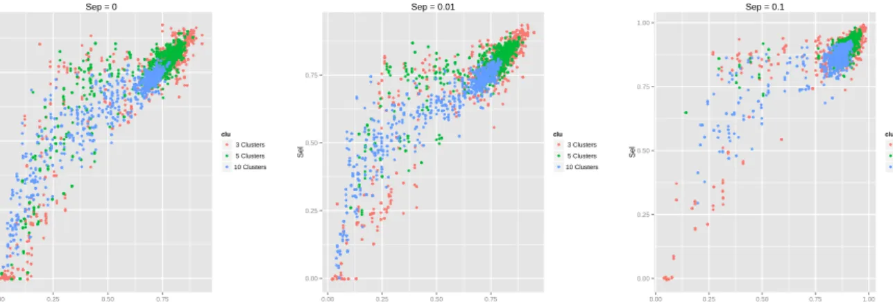
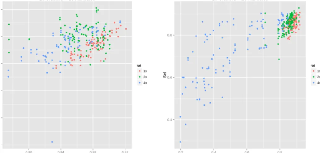
Figure 4 compares the similarity to the true labels of the partition with only the selected at-tributes, with the similarity of the partition obtained with all the attributes. Each graphic compares clusters with 3, 5 and 10 partitions with different number of attributes and different ratio of irrelevant attributes. Separation values are 0, 0.01 and 0.1.

Results show that the larger is the cluster separation, the closer is the partition obtained with only the selected attributes to the true partition. This improvement is obtained even when the partition with all the attributes is not so good. It also can be observed a tendency to obtain a better partition after the selection even when clusters are highly overlapped. For similarities under 0.75 a large number of clusterings are largely improved beyond the similarity of the partition with all attributes. This means that a very good reference partition is not strictly necessary for selecting attributes.

The distribution of the similarity of the partitions to the true partition with and without attribute selection also is affected by cluster separation. In figure 5 is represented the distribution of similarities to the true partition for the three values of cluster separation. The graphic shows that the similarity to the true partition is higher when attributes are selected. This difference of distribution is reduced with the cluster separation.

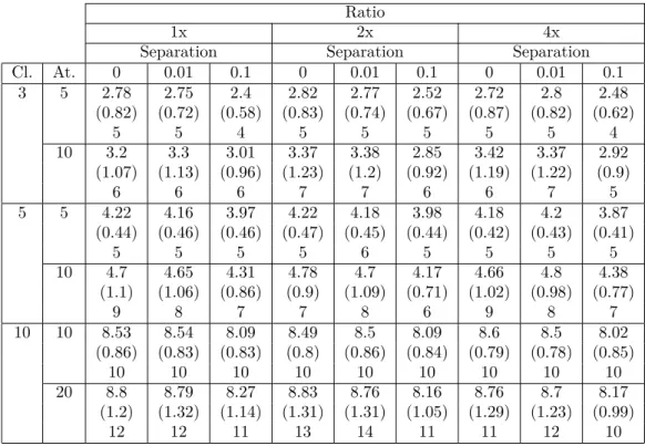
Finally tables 1 and 2 show the number of selected attributes and the irrelevant attributes in-cluded in the set of selected attibutes for different number of clusters, number of attributes, ratio of irrelevant attributes and cluster separation. These tables show the mean, the standard deviation and the maximum value.