This is a repository copy of
Joint Hypergraph Learning and Sparse Regression for Feature
Selection
.
White Rose Research Online URL for this paper:
http://eprints.whiterose.ac.uk/102293/
Version: Accepted Version
Article:
Zhang, Zhihong, Bai, Lu, Liang, Yuanheng et al. (1 more author) (2016) Joint Hypergraph
Learning and Sparse Regression for Feature Selection. Pattern Recognition. pp. 291-309.
ISSN 0031-3203
https://doi.org/10.1016/j.patcog.2016.06.009
Reuse
Unless indicated otherwise, fulltext items are protected by copyright with all rights reserved. The copyright exception in section 29 of the Copyright, Designs and Patents Act 1988 allows the making of a single copy solely for the purpose of non-commercial research or private study within the limits of fair dealing. The publisher or other rights-holder may allow further reproduction and re-use of this version - refer to the White Rose Research Online record for this item. Where records identify the publisher as the copyright holder, users can verify any specific terms of use on the publisher’s website.
Takedown
If you consider content in White Rose Research Online to be in breach of UK law, please notify us by
Joint Hypergraph Learning and Sparse Regression for
Feature Selection
Zhihong Zhanga, Lu Baib,∗, Yuanheng Lianga, Edwin Hancockc
aXiamen University, Xiamen, China
bCentral University of Finance and Economics, Beijing, China.
cUniversity of York, York, UK.
Abstract
In this paper, we propose a uniÞed framework for improved structure estimation and feature selection. Most existing graph-based feature selection methods utilise a static representation of the structure of the available data based on the Laplacian matrix of a simple graph. Here on the other hand, we perform data structure learning and feature selection simultaneously. To improve the estimation of the manifold representing the structure of the selected features, we use a higher order description of the neighbour-hood structures present in the available data using hypergraph learning. This allows those features which participate in the most signiÞcant higher order relations to be se-lected, and the remainder discarded, through a sparsiÞcation process. We formulate a single objective function to capture and regularise the hypergraph weight estimation and feature selection processes. Finally, we present an optimization algorithm to re-cover the hyper graph weights and a sparse set of feature selection indicators. This process offers a number of advantages. First, by adjusting the hypergraph weights, we preserve high-order neighborhood relations reßected in the original data, which cannot be modeled by a simple graph. Moreover, our objective function captures the global discriminative structure of the features in the data. Comprehensive experiments on 9 benchmark data sets show that our method achieves statistically signiÞcant improve-ment over state-of-art feature selection methods, supporting the effectiveness of the proposed method.
∗Corresponding author
Email address:[email protected](Lu Bai)
*Manuscript
Keywords: Feature selection, Hypergraph learning, sparse regression
1. Introduction
Feature selection aims to locate an optimal set of features using a selection crite-rion. It is an important technique widely used in pattern analysis. It reduces data di-mensionality by removing irrelevant and redundant features, and brings about a number of immediate beneÞts, such as speeding up a data mining algorithm, improving
predic-5
tive accuracy, and enhancing comprehensibility. According to the way in which label information is utilized, feature selection algorithms can be categorized as a) supervised algorithms, b) unsupervised algorithms or c) semi-supervised algorithms. Examples of supervised feature selection algorithms include the Fisher Score (FScore) [1], similar-ity preserving feature selection (SPFS)[2], minimum redundancy maximum relevance
10
(mRMR) [3], local-learning based feature selection (LLFS) [4], robust feature selec-tion viaℓ2,1-norm minimization (L21RFS) [5] and the Trace ratio [6], which only use labeled training data for feature selection. When sufÞcient labeled training samples are to used, supervised feature selection is a reliable alternative, which selects discrim-inative features by exploiting class labels. However, labeling a large set of training
15
samples manually is unrealistic in many real-world applications. In unsupervised fea-ture selection on the other hand, there is no label information, and the feafea-tures are selected which best preserve the data similarity or manifold structure. Examples in-clude the Laplacian score (LapScore) [7], spectral feature selection (SPEC) [8], multi-cluster feature selection (MCFS) [9], joint embedding learning and sparse regression
20
(JELSR) [10]. Recent work on semi-supervised learning has indicated that it is bene-Þcial to leverage both labeled and unlabeled training data for data analysis. Motivated by the progress of semi-supervised learning, considerable effort has been devoted to semi-supervised feature selection. Recent reported algorithms include discriminative semi-supervised feature selection via manifold regularization (FS-Manifold) [11],
lo-25
cality sensitive semi-supervised feature selection (LSDF) [12], the spectral analysis of semi-supervised feature selection [13] and the noise insensitive trace ratio criterion (TRCFS)[14]. Usually, these methods use graph representations to characterize the
manifold structure.
However, there are two common problems with the aforementioned methods. First,
30
the graph construction process is independent of a speciÞc learning process. Once a graph is determined that characterizes the initial manifold structure of the data, it re-mains Þxed in the following ranking or regression steps of feature selection. Therefore, the performance of feature selection is largely determined by the effectiveness of the graph construction. A typical example is thek-nearest neighbor graph used in Locality
35
Preserving Projection (LPP) [15]. LPP Þrst constructs ak-nearest neighbor graph (in-cluding its edge weights) based on the given raw data, and then seeks an optimal linear transformation with the aim to preserve such a neighborhood graph or the geometry of a given set of data. This initial graph is based on the characterization of ÒlocalityÓ which is unnecessary to be optimal, since it is difÞcult to set the parameters in advance
40
(e.g., the neighborhood size and heat kernel width). In fact, these parameters have a signiÞcant impact on the ultimate performance of the algorithm. Second, in many situations the graph representation can lead to a substantial loss of information. This is because in real-world problems objects and their features tend to exhibit multiple relationships rather than simple pairwise ones. For example, consider the problem of
45
classifying faces which are viewed under different lighting conditions. See Fig. 1 for an illustration. It is well known that images of the same objects may appear drastically different under different lighting conditions [16, 17]. In this scenario, the pairwise similarity measures for images of the same person may exhibit signiÞcant random-ness. This misleading result is due to the fact that the set of images of a Lambertian
50
surface under arbitrary lighting lies on a 3D subspace in the image space [18] where multiple relationships exist. As a result, higher order relations cannot be meaningfully characterized by pairwise similarity measures.
A natural way of remedying the information loss described above is to represent the data set as a hypergraph instead of a graph. Hypergraph representations allow
ver-55
tices to be multiply connected by hyperedges and can hence capture multiple or higher order relationships between features. Due to their effectiveness in representing mul-tiple relationships, hypergraph based methods have been applied to various practical problems, such as partitioning circuit netlists [19], clustering [20, 21], clustering
cate-Figure 1: Shown above are images of Þve persons under varying illumination conditions. Is it possible to group them into clusters based on pairwise similarity measure?
gorial data [22], and image segmentation [23]. For multi-label classiÞcation, Sun et al.
60
[24] construct a hypergraph to exploit the correlation information contained in differ-ent labels. In this hypergraph, instances correspond to the vertices and each hyperedge includes all instances annotated with a common label. With this hypergraph represen-tation, the higher-order relations among multiple instances sharing the same label can be explored. Following the theory of spectral graph embedding [25], they transform the
65
data into a lower-dimensional space through a linear transformation, which preserves the instance-label relations captured by the hypergraph. The projection is guided by the label information encoded in the hypergraph and a linear Support Vector Machine (SVM) is used to handle the multi-label classiÞcation problem. Huang et al. [26] used a hypergraph cut algorithm [21] to solve the unsupervised image categorization problem,
70
where a hypergraph is used to represent the complex relationships between unlabeled images based on shape and appearance features. SpeciÞcally, they Þrst extract regions of interest (ROI) for each image, and then construct hyperedges among images based on shape and appearance features in their ROIs. Hyperedges are deÞned as either a) a group formed by each vertex (image) or b) its k-nearest neighbors (based on shape
75
or appearance descriptors). The weight of each hyperedge is computed as the sum of the pairwise afÞnities within the hyperedge. In this way, the task of image
categoriza-tion is transferred into a hypergraph particategoriza-tion problem which can be solved using the hypergraph cut algorithm.
One common feature of these existing hypergraph representations is that they
ex-80
ploit domain speciÞc and goal directed representations. SpeciÞcally, most of them are conÞned to uniform hypergraphs where each of the hyperedges have the same cardinal-ity and therefore do not lend themselves to generalization. The reason for this lies in the difÞculty in formulating a nonuniform hypergraph in a mathematically elegant way for the purpose of computation. There has yet to be a widely accepted and consistent
85
way for representing and characterizing nonuniform hypergraphs, and this remains an open problem when exploiting hypergraphs for feature selection.
To address these shortcomings, an effective method for hypergraph construction is needed, such that the ambiguities of relational order can be overcome. In this paper, we improve the hypergraph construction approach presented above using a sparse
repre-90
sentation model. SpeciÞcally, a hypergraph is constructed using each sample as a node, and a hyperedge includes a sample and its correlated samples, with the corresponding non-zero elements extracted in the sparse vector. Instead of generating a single hy-peredge for each sample, we generate a group of hyhy-peredges by varying regularization parameter values to give different sparsity solutions of the model. This makes our
ap-95
proach much more robust than previous hypergraph methods, because we do not need to tune the neighborhood size as a parameter. However, with this hypergraph construc-tion approach, a large number of remaining hyperedges are generated with redundancy. In addition, they have different effects in classiÞcation accuracy. For example, hyper-edges that are generated from samples close to the classiÞcation boundary may link
100
samples from different classes. Since samples connected by a hyperedge are expected to be from the same class, the hyperedges that link samples from different classes will be less informative or may even have derogatory effects. Therefore, in order to modulate the effects of different hyperedges, we place a regularizer on the hyperedge weights. In this way, the effects of different hyperedges can be adaptively modulated
105
and useless hyperedges can be discarded (i.e., the weights of redundant hyperedges will be 0), and thus, we can select the most effective hyperedges.
learning and feature selection simultaneously. The structures are adaptively learned from the results of hypergraph learning, and the informative features are selected to
110
preserve the reÞned structures of data. The hypergraph can well keep high-order neigh-borhood relationship reßected by the original data, which cannot be modeled by a simple graph. Moreover, rather than just targeting the locality preserving power char-acterized by hypergraph learning, our objective function also considers global discrim-inative structure of data. Concretely, global discrimdiscrim-inative information in our
frame-115
work is preserved by exploiting the underlying pairwise sample similarity. The sample similarity measure may introduce the discriminative information when the data labels are known. Comprehensive experiments on seven benchmark data sets show that our method achieves statistically signiÞcant improvement over state-of-art feature selection methods, suggesting the effectiveness of the proposed method.
120
2. Related Work
In this section, we Þrst establish a list of the main notations used in the paper and summarized in Table.1. Then, we review some of the well-known algorithms for learning-based feature selection, all of which are closely related to our proposed method.
125
1) LapScore: Laplacian score [7] uses a k-nearest neighbor graph to model the local geometric structure of the data and selects the features most consistent with the graph structure. Consider a datasetX = [x1, . . . , xn]T, in order to approximate the
manifold structure of the dataset, ak-nearest neighbor graph is built, which contains an edge with weightwij
g betweenxi andxj ifxi is among thek nearest neighbors ofxj or conversely. There are different similarity based methods that can be used to determine the edge weights. In general, the Euclidean distance is widely used as similarity measure. Therefore, the elementwij
g of the weight matrixWgcan be deÞned as below, wij g = ⎧ ⎨ ⎩ e−∥xi−xj∥ 2
t , ifxiandxjare neighbors
0, otherwise.
. (1)
wheretis a suitable constant. A feature that is consistent with the graph structure can be thought of as the one for which two data points are close to each other if and only
Table 1: Important notations used in this paper and their deÞnitions
d The dimension of input data, i.e. the number of all features of input data.
n The number of data points. NoF The number of selected features.
k Dimensionality of embedding. m The number of hyperedges.
l The number of selected labeled data out of all dataX.
X X= [x1, . . . , xn]T ∈ ℜn×dis the input data matrix. Each rowxi∈ ℜd
denotes a data point, fori= 1, . . . , n.
Wg Wgis the weight matrix of graph where each edge weigh is represented
bywij
g. Here we assumewijg is symmetric wherewgij=wjig
fr fr = (fr1, . . . , frn)T ∈ ℜn is ther-th feature vector of data (r =
1, . . . , d). It is also ther-th column of the data matrixX, i.e.,X =
[f1, . . . , fd].
D Dis the diagonal degree matrix of graph whereDii=$ jwijg
Y Y= [y1, y2, . . . , yn]T ∈ ℜn×kis the data matrix of embedding W W= [w1, w2, . . . , wk]∈ ℜd×kis the transformation matrix De The diagonal matrix of the hyperedge degrees
Dv The diagonal matrix of the hypergraph vertex degrees H The incidence matrix of the hypergraph
WH The diagonal weight matrix and its(i, i)-th element is the weight of the
i-th hyperedge
ˆ
LH The normalized Laplacian matrix of hypergraph S S∈ ℜd×kis the sparse transformation matrix
A A∈ ℜl×nis a binary selection matrix. It selects the labeled data out of all dataX
K Kis a predeÞned similarity matrix.
w(e) The weight of hyperedgee δ(e) The degree of the hyperedgee
if there is an edge between these two points. Letfridenote thei-th sample of ther-th feature andfr = (fr1, . . . , frn)T. To select a good feature, we need to minimize the following objective function:
130 SCLs= $ ij(fri−frj)2wijg V ar(fr) . (2)
whereV ar(fr)is the estimated variance of ther-th feature. Features with larger vari-ance are preferred, as they are expected to have more representational power. Given
Wg, its corresponding degree matrix Dii = $
jwgij and Laplacian matrix L =
D−Wg, the variance of weight data can be calculated based onDwhich models
the importance of the data points.
V ar(fr) = ˜frTDf˜r, (3) where ˜ fr =fr− fT rD1 1TD11, (4)
Here, we center the data by subtracting the mean from each featurefrusing Equation (4). This is done to prevent a non-zero constant vector such as1to be assigned a zero
Laplacian score, since such a feature obviously does not contain any information. For a good feature, the largerwij, the smaller(fri−frj), and thus it is easy to see that,
%
ij
(fri−frj)2wijg = 2frTLfr= 2 ˜frTLf˜r, (5)
Finally, the Laplacian score of ther-th feature is reduced to
SCLs(fr) = ˜ fT rLf˜r ˜ fT r Df˜r , (6)
2) MCFS and MRSF: MCFS and MRSF are learning based feature selection
meth-135
ods that Þrst compute an embedding and then use regression coefÞcients to rank each feature. In the Þrst step, both methods compute a low dimensional embedding rep-resented by the co-ordinate matrixY. One simple way in deriving low dimensional embedding is to use the Laplacian Eigenmap (LE) [27], a well known dimensional-ity reduction method. Denote byY = [y1, y2, . . . , yn]T andˆyias transpose of the
i-th row ofY. The idea common to both MCFS and MRSF is to regress allxi toyˆi.
Their differences are used to determine sparseness constraints. MCFS [9] usesℓ1-norm regularization and can be regarded as solving the following problems in sequence:
Y =arg min YYT=Itr( YLYT) W=argmin W ∥ XW−Y∥2 2+α∥W∥1 (7) Similarly, MRSF Þrst computes the embedding by Eigen decomposition of the graph Laplacian and then regression is withℓ2,1-norm regularization. In other words, MRSF 145
can be regarded as solving the following two problems in sequence:
Y =arg min YYT=Itr( YLYT) W=argmin W ∥ XW−Y∥2 2+α∥W∥2,1 (8) MCFS and MRSF employ different sparseness constraints, i.e.,ℓ1andℓ2,1 respec-tively, in constructing a transformation matrix which is used for selecting features. Nevertheless, the low dimensional embedding, i.e.,Y, is determined in the Þrst step
and remains Þxed in the subsequent ranking or regression step. As a result the
per-150
formance of feature selection is largely determined by the effectiveness of graph em-bedding. However, it would be better to learn a graph structure closely linked with the feature selection process.
3) JELSR [28]: Instead of simply using the graph Laplacian to characterize high dimensional data structure and then performing regression, JELSR (joint embedding learning and sparse regression) uniÞes embedding/learning and sparse regression steps in constructing a new framework for feature selection :
(W, Y) =arg min
W,YYT=Itr(
YLYT) +β(∥XW−Y∥2
2+α∥W∥2,1) (9) whereα andβ are balance parameters. The objective function in Eq.(9) is convex with respect toWandY. As a result,WandY can be updated in an alternative
155
way. As we can see from Eq.(29) in [28], the sparse regression of objective function, i.e. the value ofW, also affects the low dimensional embedding, i.e.,Y. Alternative
methods, such as MCFS and MRSF, simply minimizetr(YLYT). Although JELSR
on the transformed data, without making the best use of the original data and the graph
160
edge weights also not learned by the algorithm. This easily leads to the instability performance, especially when encountering a ÒbadÓ transformation matrix.
4) LPP [15]: LPP (locality preserving projection) constructs a graph by incorpo-rating neighborhood information derived from the data. Using the graph Laplacian, a transformation is computed to map the data into a subspace by optimally maintaining the local neighborhood information. LPP optimizes a linear transformationW
accord-ing to min W n % i,j=1 ∥xiW−xjW∥2wijg s.t. WTXTDXW= 1 (10) where wij
g is the graph edge weight which can be computed by Eq.1 and Dii = $
jwgij. The basic idea underlying LPP is to Þnd a transformation matrixW, which transforms the high-dimensional dataXinto a low-dimensional matrixXW, so as to
165
maximally preserve the local connectivity structure ofXwithXW. Minimizing (10)
ensures that, ifxiandxjare close, and as a resultxiWandxjWare close too. As described above, LPP seeks a low-dimensional representation with the purpose of preserving the local geometry in the original data. However, such Òlocality geome-tryÓ is completely determined by the artiÞcially constructed neighborhood graph. As
170
a result, its performance may drop seriously if given a ÒbadÓ graph. Therefore, it is better to optimize the graph and learn the transformation simultaneously in a uniÞed objective function.
Our proposed method can be discriminated from the previous methods in the fol-lowing senses:(1) Our propose method selects features to respect both the global and
175
local manifold structure, while most previous feature selection methods only incorpo-rates the local manifold structure; (2) The local structure in previous methods is based on ak-nearest neighbor graph, while our proposed method learns a hypergraph, which can model high-order neighborhood relationship reßected by the original data. (3) JELSR [28] iteratively performs spectral embedding for clustering and sparse spectral
180
matrix) is not changed during iterations. Our proposed method can adaptively improve the local structure characterization using hypergraph learning.
3. Hypergraph Learning
In this section, we review the deÞnitions of hypergraphs and hypergraph Laplacian.
185
Then, we present our hypergraph construction and learning method.
3.1. Hypergraph Fundamentals
A hypergraph is deÞned as a tripletGH = (V, E, w), whereV ={1, . . . , n}is the node index set,Eis a set of non-empty subsets ofV or hyperedges andwis a weight function which associates a real value with each edge. A hypergraph is a generalization
190
of a graph. Unlike graph edges which consist of pairs of vertices, hyperedges are arbitrarily sized sets of vertices. Each hyperedgeeis assigned a positive weightw(e). The degree of a hyperedgee, denoted asδ(e), is the number of vertices ine. For a vertexv∈V, the degree is deÞned to bed(v) =$
v∈e,e∈Ew(e). The diagonal matrix representations forδ(e),d(v),w(e)are denoted byDe,Dv andWH, respectively.
195
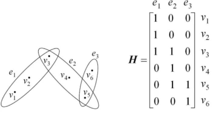
Examples of a hypergraph are shown in Fig. 2(a). For the hypergraph, the vertex set is
V ={v1, v2, v3, v4, v5, v6}, where each vertex represents a sample, and the hyperedge set isE = &
e1 = {v1, v2, v3}, e2 = {v3, v4, v5}, e3 = {v5, v6}'. The number of vertices constituting each hyperedge represent the order of the relationship between samples.
200
The hypergraphGH can be represented by a vertex-edge incidence matrixH ∈
R|V|×|E|(see Fig. 2(b)) is deÞned as follows:
h(v, e) = ⎧ ⎨ ⎩ 1, ifv∈e 0, otherwise. (11)
According to the deÞnition ofH,d(v) =$
e∈Ew(e)h(v, e)andδ(e) = $
v∈Vh(v, e).
3.2. Hypergraph Laplacian
Although the incidence matrix Hcan fully describe the characteristics of a
(a) Hypergraph Example (b) Incidence Matrix
Figure 2: An Example of Hypergraph.
vertex-to-vertex relationships. To obtain a vertex-to-vertex representation, we need to
205
establish the adjacency matrix and Laplacian matrix for a hypergraph. To achieve this goal, one possible method is to construct a graph with edges weighted by the quotient of the corresponding hyperedge weight and cardinality, e.g., clique expansion [29] and star expansion [29]. As an alternative, one approach is to adopt a matrix representation determined from the adjacency matrix and the associated Laplacian matrix for a
hyper-210
graph, e.g. the normalized Laplacian [21]. In this paper, we adopt the method proposed in [21] to build the hypergraph Laplacian. SpeciÞcally, the normalized Laplacian ma-trix of a hypergraph is deÞned asLˆH=I|V|−D−12
v HWHD−e1HTD
−1 2
v , whereDv is the diagonal vertex degree matrix whose diagonal elementd(vi)is the summation of thei-th row ofH, andDeis the diagonal edge degree matrix whose diagonal element
215
δ(ej)is the summation of thej-th column ofH.
3.3. Hypergraph Construction and Learning
For our hypergraph construction, we regard each sample in the data set as a vertex on hypergraphGH = (V, E, w), whereV = {x1, x2, . . . , xn}is the vertice set. In-spired by the recent developments on sparse representation andℓ1-regularized models [30], we propose to generate hyperedges by linking correlated samples. SpeciÞcally, each sample can be regarded as a response vector, and can be estimated by a linear
combination of remainingn−1samples, i.e.,
xi=Piαi+εi, i= 1,2, . . . , n (12)
wherePi = [x1, x2, . . . , xi−1,0, xi+1, . . . , xn] denotes a data set including all the samples except thei-th sample (we put 0 in its location), andαi essentially contains the combination coefÞcients for different samples in approximatingxi, andεi ∈ ℜn is a noise term. A natural method for determining sparse solutions ofαiis formed by solving the following problem:
min
αi
∥xi−Piαi∥2+λ∥αi∥1 (13)
whereλ > 0is a regularization parameter controlling the sparsity ofαi. Due to the nature of theℓ1-norm penalty, some coefÞcients will be shrunk to zero ifλis large enough. In this case, we can generate a hyperedge containing the most correlated
220
samples (corresponding to the non-zero coefÞcients inαi) with respect toxi. Different
λvalues correspond to different sparsity solutions. So instead of generating a single hyperedge for each samplexi, we generate a group of hyperedges by varying the value ofλover a speciÞed range. SpeciÞcally, in our experiments, we varyλfrom0.1to0.9
with an incremental step of0.1.
225
With this hypergraph construction approach, a large set of remaining hyperedges are generated with redundancy. In addition, they have varying effects on the classi-Þcation. For example, several hyperedges that are generated from samples close to the classiÞcation boundary and they link samples from different classes. Therefore, an effective method for modulating the effects of different hyperedges is needed, such
230
that the weights of redundant hyperedges will be 0, and allowing to select the effective hyperedges.
The importance of preserving local geometric data structure has been well recog-nized in the recent literature on dimensionality reduction [31] [32] [15] [33]. The local geometric structure of data refers to the local neighborhood relationships for a set of a
235
dataset, which can be characterized through theknearest neighbors of each sample. By evoking by the principle that nearby points should have similar properties, we deÞne a
regularizer on the hypergraph: Ω= 12 $ e∈E $ xi,xj∈V w(e)h(xi,e)h(xj,e) δ(e) ×(xiS−xjS)2 = STXTLˆ HXS = STXT(I |V|−D −1 2 v HWHD−e1HTD −1 2 v )XS (14)
whereSis a linear transformation matrix. The weight of the hyperedgeeis assigned
a term2δ1(e) $ xi,xj∈V(e)
(xiS−xjS)2. Here,V(e)is used to denote the set of vertices connected to hyperedgee. As a result, this term measures the feature smoothness on the samples inV(e). Intuitively, hyperedges connecting to the samples from the same class are informative by minimizing (14) with respect toWH. We ensure that, ifxi
andxjare close, thenxiSandxjSwill also be close. Therefore, we use the following objective function to learn the weights of the hyperedgesWH
min WH tr(STXTLˆHXS) +γ∥diag(WH)∥2 s.t. $m j=1 WHj= 1, WHj ≥0, j= 1, . . . , m (15)
wheremis the number of hyperedges and diag(WH)indicates the diagonal vector of WH, i.e.,(W1
H, WH2, . . . , WHm). In order to control the model complexity motivated
240
by the success of sparse learning, we add two constraints m $ j=1
WHj = 1andWHj ≥0in (15). In particular, the Þrst constraint Þxes the summation of the weights. The second constraint avoids negative weights. Thus, we can see that the solution ofWHis on a
simplex and enjoys the property of sparseness, i.e., the weights assigned to redundant hyperedges will be set to 0.
245
4. Proposed Framework for Feature Selection
Turning our attention to the task of feature selection, we expect that the trans-formation matrixSin (15) satisÞes the sparsity property for feature selection. More
concretely, we expect that only a few elements inSare nonzero. As a result the
cor-responding featuresXSare selected since these features are sufÞcient to preserve the
regularizer to enforce row sparsity ofS, and thus has the effect of feature selection
and helps to avoid selecting redundant features. This paper introduces a novel fea-ture selection framework: joint hypergraph learning and sparse regression (referred to as JHLSR). Rather than simply targeting the locality preserving power characterized by hypergraph learning, our proposed model also accommodate the sample similarity structure which can be computed using a predeÞned similarity measure. In order fulÞll this goal, we propose to unify hypergraph learning and sample similarity preserving in forming a new framework as
min S,WH ∥(AXS)(AXS)T−K∥2 F+µtr(S TXTLˆ HXS) +λ∥S∥2,1+γ∥diag(WH)∥2 s.t. $m j=1 WHj= 1, WHj ≥0, j= 1, . . . , m (16)
whereA ∈ ℜl×nis a binary selection matrix andKis a predeÞned similarity matrix.
It selects the labeled data out of all dataXwhen both labeled and unlabeled data are
available.S∈ ℜd×kwheredis the number of features inXandkdenotes the
dimen-sions of the transformed data. ∥·∥F denotes the Frobenius matrix norm and∥·∥2,1is theℓ2,1-norm ofS. The Þrst term in (16) stands for the global structure preservation by emphasizing the pairwise sample similarity, while the second term exploits the local geometric structure of data. The third term is theℓ2,1-norm regularization term, which is added to promote row-sparsity. The last term is the diagonal vector of hyperedge weightWHand enjoys the sparse property, i.e., the weights of useless hyperedges will
be set to 0. To be more speciÞc, the Þrst term aims to selectk(k < d) features, based on which best preserves the sample similarity as speciÞed by a predeÞned similarity ma-trixK. Here,Kis constructed using the Fisher Kernel in supervised learning [2] and
by a Gaussian Kernel in unsupervised learning. However,∥(AXS)(AXS)T−K∥2 F is not convex with respect toS. To solve this problem, the method in [2] addresses the
following convex optimization problem instead:
min
S ∥
AXS−Φ∥2
F+λ∥S∥2,1 (17) whereΦis obtained by decomposingKasK=ΦΦT. Note that∥S∥
2,1is convex. Nevertheless, its derivative does not exist whensˆi= 0fori= 1,2, . . . , d. Therefore,
we use the deÞnitiontr(STUS) = ∥S∥
2,1/2in [28] whenˆsiis not equal to 0. The
U∈ ℜd×dis diagonal withi-th diagonal element where
Uii=
1
2∥ˆsi∥2
(18)
Based on the deÞnitions in (17) and (18), our proposed objective function (16) can be rewritten as min S,WH ∥AXS−Φ∥2 F+µtr(STXTLˆHXS) +λtr(STUS) +γ∥diag(WH)∥2 s.t. $m j=1 WHj= 1, WHj ≥0, j = 1, . . . , m (19)
From (19), it is clear that the proposed objective function has a regularizer on the hyperedge weights and simultaneously optimizes both the transformation matrixSand
the hyperedge weightsWH. In this way, the effects of different hyperedges can be
adaptively regulatedÕ. For those hyperedges that are informative, higher weights will
250
be assigned. In addition, our method sparsiÞes the transformation matrixS, i.e., it
optimizesSby maximally preserving both the local geometrical structure of the data
characterized byˆLHand the sample similarity of the labeled data characterized byK.
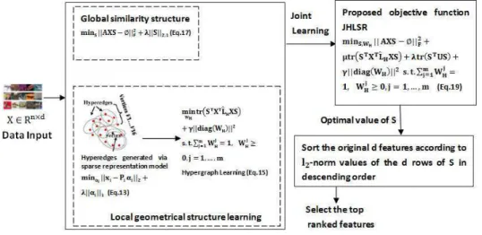
Figure 3: Flowchart of the proposed method
pro-pose a global and local structure preservation framework for feature selection which
255
integrates both global sample similarity structure and local geometrical structure to conduct feature selection (see Eq.19). Concretely, global discriminative information in our framework is preserved by exploiting the underlying sample similarity (see Eq.17). The sample similarity measure may introduce the discriminative information when the data labels are known. Local geometrical structure of data refers to the local
neigh-260
borhood relationship of a dataset, which can be captured by the results of hypergraph learning (see Eq.15). SpeciÞcally, a hypergraph is constructed using each sample as a node, and a hyperedge includes a sample and its correlated samples, with the corre-sponding non-zero elements extracted in the sparse vector (see Eq.13).
5. Optimization Algorithm
265
The initial value for each hyperedge weight is set according to the rules given in [34]. First, the |V|×|V| afÞnity matrix A is calculated according to Aij =
exp(
−∥vi−vj∥2
σ2
)
whereσis the average distance among all vertices. Then, the initial weight for each hyperedge isWi
H = $
vj∈eiAij. To obtain the global minimal
solu-tion of (19), we need an iterative and interleaved optimizasolu-tion process, which can be
270
summarized as in Algorithm 1. In each iteration step, the sparse matrixSis calculated
with the current valueWH, as in equation (21). The diagonal matrixWHis updated
based on the merely calculated value ofSas in equation (27). After obtainingWH,
we then update the normalized Laplacian matrixLˆHin (23).
We Þrst ÞxWHand solve forS. In other words, we need to solve the following
subproblem:
min
S ∥
AXS−Φ∥2
Taking the derivative with respect toSand setting it to zero, we have ∂ ∂S * ∥AXS−Φ∥2 F +µtr(STXTLˆHXS) +λtr(STUS) + = 0 ⎧ ⎪ ⎪ ⎪ ⎪ ⎪ ⎪ ⎪ ⎪ ⎪ ⎨ ⎪ ⎪ ⎪ ⎪ ⎪ ⎪ ⎪ ⎪ ⎪ ⎩ ∂ ∂S∥AXS−Φ∥ 2 F =2(XTATAX)S−2ATXTΦ, ∂ ∂Str(S TUS) =2US, ∂ ∂Str(S TXTLˆ HXS) =2(XTLˆHX)S. S=-XT(ATA+µLˆ H)X+λU .−1 ATXTΦ (21)
We then ÞxSand solve forWH. The subproblem becomes
min WH µtr(STXTLˆHXS) +γ∥diag(WH)∥2 (22) Let ˆ LH=I|V|−D−12 v HWHD−e1H TD−12 v (23)
Then solving the minimization problem in Eq.(22) with respect toWHis equivalent
to the following problem,
min WH / −µtr(STXTD −1 2 v HWHD−e1HTD −1 2 v XS) +γ∥diag(WH)∥2 0 s.t. m $ j=1 WHj= 1, WHj ≥0, j= 1, . . . , m (24) SinceWHandD−1
e are both diagonal matrices, we letR=STXTD
−1
2
v HwhereR is the matrix[rT
1, . . . , rmT]T andri = [r1i, r2i, . . . , rmi ]. The Þrst term appearing in Eq.(24) can be written as
tr(STXTD −1 2 v HWHD−e1HTD −1 2 v XS) =tr(RWHD−e1RT) (25)
In Eq.(25), its matrix form becomes tr(RWHD−1 e R T ) =tr(R∗ ⎡ ⎢ ⎢ ⎢ ⎣ W1 H 0 0 0 . .. 0 0 0 Wm H ⎤ ⎥ ⎥ ⎥ ⎦ ∗ ⎡ ⎢ ⎢ ⎢ ⎣ δ(e1)−1 0 0 0 . .. 0 0 0 δ(em)−1 ⎤ ⎥ ⎥ ⎥ ⎦ ∗RT) =W1 H -%m i=1 (r1 i)2 . δ(e1)−1+· · ·+WHm -%m i=1 (rm i )2 . δ(em)−1 Therefore, the minimization problem in Eq.(24) can be rewritten as
min WH 7 −µ 8 W1 H -%m i=1 (r1 i)2 . δ(e1)−1+· · ·+WHm -%m i=1 (rm i )2 . ∗δ(em)−1 9 +γ∥diag(WH)∥2 : s.t. $m j=1 WHj= 1, WHj ≥0, j= 1, . . . , m (26)
We use the coordinate descent algorithm to solve the above minimization problem. At each iteration, two elements are selected for updating, and the remainder are Þxed. For example, in an iteration, thep-th and theq-th elements, i.e.,WHp andWHq, are selected. According to constrain
m $ j=1
WHj = 1, the summation ofWHp andWHq will not change after this iteration step. Hence, we have
⎧ ⎪ ⎪ ⎪ ⎪ ⎪ ⎪ ⎪ ⎪ ⎪ ⎪ ⎪ ⎪ ⎨ ⎪ ⎪ ⎪ ⎪ ⎪ ⎪ ⎪ ⎪ ⎪ ⎪ ⎪ ⎪ ⎩ WHp∗= 0, WHq∗=WHp +WHq, if 2γµ(WHp +WHq) +(Sq−Sp)≤0 WHp∗=WHp +WHq, WHq∗= 0, if 2γ µ(W p H+W q H) +(Sp−Sq)≤0 WHp∗= (2γ/µ)(W p H+W q H)+(Sq−Sp) 4γ/µ , else WHq∗=WHp +WHq −WHp∗ (27) whereSp = −( $mi=1(r p i)2 ) ∗δ(ep)−1andSq = −( $mi=1(r q i)2 ) ∗δ(eq)−1. Note 275
that, in the Þrst line of Eq.(27), we can see thatWHp∗will be set to 0. This indicates the solution ofWH has the potential to be sparse, i.e., redundant hyperedges will be removed.
After the optimal value ofSis obtained, we then sort the originald features
ac-cording toℓ2-norm values of thedrows ofSin descending order, and then select the 280
top ranked features.
Algorithm 1:Joint Hypergraph Learning and Sparse Regression (JHLSR)
Input:X,K,Aand regularization parameterµ,λandγ.WHwith initial values,
hypergraph normalized LaplacianˆLH, the matricesDv,DeandH
accordingly.
Output: the otpimalWHand sparse matrixS
Step 1: Sparse matrixSupdate. ;
1: repeat
2: computeSt1+1by Eq.21;
3: calculate the diagonal matrixUt1+1, where thei-th diagonal element is
1 2∥sˆt1 +1 i ∥2 ; 4: t1=t1+ 1; 5: untilconvergence;
Step 2:WHupdate. Update the weightsWHwith the iterative coordinate
descent method introduced in (27) ;
Step 3:LˆHupdate. Update the normalized Laplacian matrixLˆHin (23)
accordingly ;
Step 4: Lett2=t2+ 1. ift2> T, quit iteration and output the results, otherwise go toStep 1.
6. Convergence and Complexity Analysis
In this section, we will analyze the properties of the JHLSR algorithm according to three criteria. We Þrst provide the convergence analysis and then discuss computational complexity and parameter determination problems.
285
6.1. Convergence Proof
Since we have solve JHLSR in an alternative way, we would like to show its conver-gence behavior. The converconver-gence ofAlgorithm 1can be guaranteed if the following
properties be satisÞed.
Theorem 1: The iterative procedure, i.e.,Step 1inAlgorithm 1, will monotonically
290
decrease the objective function value in Eq.20.
Theorem 2: WhenSis Þxed,Step 2inAlgorithm 1will monotonically decrease the
objective function value in Eq.19.
Proofs: The proof of Theorem 1 and Theorem 2 are provided in the Appendix A and Appendix B respectively.
295
From Theorem 1 and Theorem 2, we can see that the iterative procedure inAlgorithm 1
will monotonically decrease the objective function and converge to a global optimum. The following experiments also conÞrm that the proposed method converges rapidly, typically with a number of iterations is less than 4.
6.2. Complexity Analysis 300
At each iteration, the main computation ofStep 1inAlgorithm 1is to solve the
d×dmatrix inverse problem in Eq.21. For many feature selection tasks, the feature dimensionalitydis much larger than the number of samplesn. The inverse of a large matrix can considerably increase the computational cost. According to [5], we have the following identity:
305 -XT(ATA+µLˆH)X+λU .−1 XT=ΩXT -(ATA+µLˆH)XΩXT+I .−1 (28)
whereΩ = 1λU−1andI is ann×nidentity matrix. From Eq.28, we can convert ad×dmatrix inverse problem to ann×none. In doing so, the time complexity of
Step 1inAlgorithm 1at each iteration isO(
min(n, d)3)
. And the computational cost ofStep 2isO(m2), wheremis the number of hyperedges. The computational cost of the hypergraph construction process in Eq.13 isO(r3+n2), whereris the number 310
of nonzero coefÞcients inα. Thus, the computational complexity ofAlgorithm 1is
max;O(
min(n, d)3)
, O(m2), O(r3+n2)<.
6.3. Parameter Determination
A parallel issue to optimizing the JHLSR algorithm is selecting optimal values of the parametersµ,λandγ. The parameterλandγ are regularization parameters
controlling the sparsity ofSandWH, and the parameterµis used to trade off the
importance of data similarity preservation and local geometric structure preservation. In order to assign an appropriate value ofµ, we employ a cross-validation procedure forµestimation. In addition, another two parameters, i.e., λandγ are empirically determined by grid search.
320
7. Experiments and Comparisons
In this section, we discuss the merits and limitations of the proposed feature se-lection approach, including a convergence analysis, computational complexity, and pa-rameter determination. A comprehensive experimental study on a variety of data sets is conducted in order to compare our feature selection approach with several
state-of-325
the-art methods in supervised, unsupervised, and semi-supervised modes.
7.1. Experimental Setting
From (16), we observe that theA∈ ℜl×nis a binary selection matrix and it selects the labeled data out of all dataXwhen both labeled and unlabeled data are available. Awill degenerate to an identity matrix when only with labeled or unlabeled data are
330
available. According to the value ofA, the objective function (19) can implement feature selection in supervised, unsupervised and semi-supervised way. Here, we refer to our proposed method in these three modalities as Sup-JHLSR, Un-JHLSR and Semi-JHLSR respectively. The initial value for each hyperedge weight is set according to the rules given in [34].
335
To demonstrate the effectiveness of the proposed approach, we conduct experi-ments on 9 benchmark data sets, i.e., a) the Prostate-GE [5], b) malignant glioma (GLIOMA) data set [35], c) SMK-CAN [36], d) COIL-20 [37], e) handwritten digit image data set MNIST [38], f) Caltech256-2000 [39], g) Scene15 [40], h) ORL [7] and i) ALLAML [5]. Table. 2 summarizes the extent and properties of each of the 9
data-340
sets. For each dataset,50%of samples are randomly selected as training data, and the remaining are treated as test data in both supervised and the unsupervised modalities. In the semi-supervised case,5%and40%samples are randomly selected as labeled and
unlabeled data, respectively, and the remaining are used as test data. We repeat this procedure 10 times and obtain 10 random partitions of the original data. The above
345
feature selection algorithms are evaluated on each partition and the averaged results are reported.
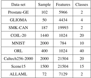
Table 2: Summary of 9 benchmark data sets
Data-set Sample Features Classes Prostate-GE 102 5966 2 GLIOMA 50 4434 4 SMK-CAN 187 19993 2 COIL-20 1440 1024 20 MNIST 2000 784 10 ORL 400 1024 40 Caltech256-2000 2000 21504 20 Scene15 1500 21504 15 ALLAML 72 7129 2 7.2. Experiment setup
In order to explore the discriminative capabilities of the information captured by our method, we use the selected features for the purpose of classiÞcation. We compare the
350
classiÞcation results from our proposed method (Sup-JHLSR, Un-JHLSR and Semi-JHLSR) with twelve representative feature selection algorithms.
For supervised learning, six alternative feature selection algorithms are selected as baselines. Compared with our proposed method Sup-JHLSR, most of these methods focus on selecting features that preserve the sample similarity, and neglect the local
355
geometric structure of data. We will brießy introduce these methods one by one. •Fscore[1]: Fisher Score is a classical feature selection algorithm. It conducts feature selection by evaluating the importance of features one by one. In contract to LapScore and SPEC, Fscore is supervised with class label.
•SPFS [2]: The basic idea of SPFS is to pursue a transformation matrix, which
transform the high-dimensional data to a low-dimensional data, to maximally preserve the global similarity structure of original data.
•mRMR [3]: mRMR is a mutual information based method which is designed to select features that have the maximal statistical dependency on the classiÞcation vari-able, while simultaneously minimizing the redundancy among the selected features.
365
•LLFS [4]: LLFS selects features which best preserve the global similarity struc-ture of the original data.
•L21RFS [5]: L21RFS shares the spirit of similarity preservation is SPFS. The major difference between L21RFS and SPFS is that the regression loss in SPFS is measured by the Frobenius norm, while theℓ2,1-norm is adopted in L21RFS.
370
•Trace ratio [6]: The trace ratio criterion locates a feature subset for which the within class pairwise afÞnities are large, while the between class separation is large.
For unsupervised learning, four alternative feature selection algorithms are selected as baselines. A commonly used criterion in these alternative methods is to select the features which best preserve the manifold structure derived from the Laplacian of a
375
graph, where the graph is constructed before hand. However, they separate the pro-cesses of learning the graph and feature ranking. In practice, the ideal graph is difÞcult to deÞne in advance. Because one needs to assign appropriate values for parameters such as the neighborhood size or the heat kernel parameter involved in graph construc-tion, the process is conducted independently of subsequent feature selection. As a result
380
the performance of feature selection is largely determined by the effectiveness of graph construction. Our proposed method Un-JHLSR performs data manifold structure learn-ing and feature selection simultaneously.The structures are adaptively learned from the results of hypergraph learning, and the informative features are selected to preserve the reÞned structures of data.
385
• LapScore [7]: LapScore selects features which can best preserve the locality relationship revealed by weight matrix of a predeÞned graph.
•SPEC [8]: SPEC is a framework for feature selection based on spectral graph theory. It Þrstly constructs a normalized graph Laplacian and then deÞnes different metrics to measure the importance of each feature. SPEC also can be regarded as an
390
•MCFS [9]: Multi-Cluster Feature Selection (MCFS) selects features by sequen-tially conducting manifold learning and spectral regression.
•JELSR [10]: which joint embedding learning with sparse regression to perform feature selection.
395
We also compare our obtained results with two state-of-art semi-supervised feature selection methods:
• LSDF [12]: Locality sensitive semi-supervised feature selection (LSDF) is a semi-supervised feature selection approach based on within-class and between-class graph construction.
400
•TRCFS [14]. Noise insensitive trace ratio criterion for feature selection (TRCFS) is a recent semi-supervised algorithm based on noise insensitive trace ratio criterion.
A 10-fold cross-validation strategy using the C-Support Vector Machine (C-SVM) [41] is employed to evaluate the classiÞcation performance. We perform the cross-validation on the test samples taken from the feature selection process. SpeciÞcally, the
405
entire sample is randomly partitioned into 10 subsets and then we choose one subset for test and use the remaining 9 for training, and this procedure is repeated 10 times. The Þnal accuracy is computed by averaging the accuracies from each of the random subsets.
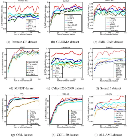
7.3. ClassiÞcation Evaluation 410
Each subÞgure shows the classiÞcation accuracy versus the number of selected features for each dataset in turn.
1)Results for the Supervised Case (Sup-JHLSR): The classiÞcation accuracies obtained with different feature subsets based on supervised learning are shown in Fig.4. From the Þgure, it is clear that our proposed method Sup-JHLSR is, by and large,
su-415
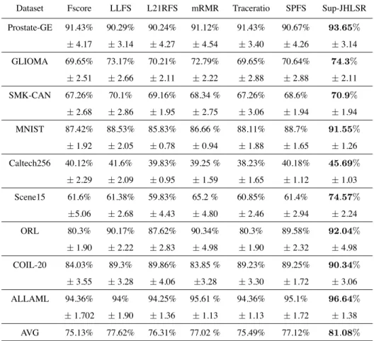
perior to the alternative supervised feature selection methods on all the 9 benchmark datasets. Following [2], Table. 3 reports the Òaggregated Ó SVM classiÞcation ac-curacy of different algorithms on each data set. The aggregated SVM classiÞcation accuracy is obtained by averaging the averaged accuracy achieved by SVM using the top 10,20,. . .,200 features selected by each algorithm. The boldfaced values are the
420
0 50 100 150 200 0.86 0.88 0.9 0.92 0.94 0.96 Prostate−GE C − SVM cl a ssi fi ca ti o n a ccu ra cy
Num of selected feature
Fscore L21RFS LLFS MRMR Sup−JHLSR SPFS Trace ratio
(a) Prostate-GE dataset
0 50 100 150 200 0.5 0.55 0.6 0.65 0.7 0.75 0.8 GLIOMA C − SVM cl a ssi fi ca ti o n a ccu ra cy
Num of selected feature Fscore L21RFS LLFS MRMR Sup−JHLSR SPFS Trace ratio (b) GLIOMA dataset 0 50 100 150 200 0.58 0.6 0.62 0.64 0.66 0.68 0.7 0.72 0.74 SMK−CAN C − SVM cl a ssi fi ca ti o n a ccu ra cy
Num of selected feature Fscore L21RFS LLFS MRMR Sup−JHLSR SPFS Trace ratio (c) SMK-CAN dataset 0 50 100 150 200 0.5 0.6 0.7 0.8 0.9 1
Num of selected feature
C − SVM cl a ssi fi ca ti o n a ccu ra cy MNIST Sup−JHLSR Trace ratio LLFS MRMR FScore SPFS L21RFS (d) MNIST dataset 0 50 100 150 200 0.32 0.34 0.36 0.38 0.4 0.42 0.44 0.46 0.48 Caltech256 C − SVM cl a ssi fi ca ti o n a ccu ra cy
Num of selected feature
Fscore L21RFS LLFS MRMR Sup−JHLSR SPFS Trace ratio
(e) Caltech256-2000 dataset
0 50 100 150 200 0.45 0.5 0.55 0.6 0.65 0.7 0.75 0.8
Num of selected feature
C − SVM cl a ssi fi ca ti o n a ccu ra cy Scene15 Sup−JHLSR Trace ratio LLFS MRMR SPFS L21RFS Fscore (f) Scene15 dataset 0 50 100 150 200 0.5 0.6 0.7 0.8 0.9 1 ORL C − SVM cl a ssi fi ca ti o n a ccu ra cy
Num of selected feature Fscore L21RFS LLFS MRMR Sup−JHLSR SPFS Trace ratio (g) ORL dataset 0 50 100 150 200 0.5 0.6 0.7 0.8 0.9 1 COIL−20 C − SVM cl a ssi fi ca ti o n a ccu ra cy
Num of selected feature Fscore L21RFS LLFS MRMR Sup−JHLSR SPFS Trace ratio (h) COIL-20 dataset 0 50 100 150 200 0.90 0.92 0.94 0.96 0.98
Num of selected feature
C − SVM cl a ssi fi ca ti o n a ccu ra cy ALLAML Sup−JHLSR SPFS L21RFS MRMR Trace ratio LLFS FScore
(i) ALLAML dataset
Figure 4: Accuracy rate vs. the number of selected features on 9 benchmark datasets by supervised learning.
The bottom row of Table. 3 shows the averaged classiÞcation accuracy for all the algorithms over the 9 datasets. Our method improved the classiÞcation accuracy by 5.95%(Fscore), 3.46%(LLFS), 4.77%(L21RFS), 4.06%(mRMR), 5.59% (Tracera-tio) and 3.96%(SPFS), respectively, compared to the averaged classiÞcation accuracy
425
of all competing methods over the 9 datasets. Meanwhile, our method gives a lower standard deviation and hence more stable than the alternatives. Overall, Fscore gives the worst performance. This may be explained by the fact that it is unable to handle feature redundancy and is prone to select redundant features. SPFS and L21RFS both select a feature subset in which the pairwise similarity between high dimensional
Table 3: Study of supervised cases: aggregated SVM classiÞcation accuracy (MEAN±STD). The last row shows the averaged classiÞcation accuracy of all the algorithms over the 9 datasets.
Dataset Fscore LLFS L21RFS mRMR Traceratio SPFS Sup-JHLSR Prostate-GE 91.43% 90.29% 90.24% 91.12% 91.43% 90.67% 93 .65% ±4.17 ±3.14 ±4.27 ±4.54 ±3.40 ±4.26 ±3.14 GLIOMA 69.65% 73.17% 70.21% 72.79% 69.65% 70.64% 74 .3% ±2.51 ±2.66 ±2.11 ±2.22 ±2.88 ±2.88 ±2.11 SMK-CAN 67.26% 70.1% 69.16% 68.34 % 67.26% 68.6% 70 .9% ±2.68 ±2.86 ±1.95 ±2.75 ±3.06 ±1.94 ±1.94 MNIST 87.42% 88.53% 85.83% 86.66 % 88.11% 88.7% 91 .55% ±1.92 ±2.05 ±0.78 ±0.94 ±1.88 ±1.65 ±1.26 Caltech256 40.12% 41.6% 39.83% 39.25 % 38.23% 40.18% 45 .69% ±2.29 ±2.09 ±0.95 ±1.59 ±1.65 ±1.12 ±1.03 Scene15 61.6% 61.38% 59.83% 65.2 % 60.85% 61.4% 74 .57% ±5.06 ±2.68 ±4.43 ±4.80 ±2.46 ±2.94 ±2.24 ORL 80.3% 90.17% 87.62% 90.34% 80.3% 89.58% 92 .04% ±1.90 ±2.22 ±2.83 ±4.98 ±1.90 ±2.32 ±4.98 COIL-20 84.03% 89.3% 89.86% 83.85 % 89.23% 89.25% 90 .34% ±3.55 ±3.28 ±4.06 ±3.28 ±3.30 ±1.72 ±3.06 ALLAML 94.36% 94% 94.25% 95.61 % 94.36% 95.1% 96 .64% ±1.702 ±1.90 ±1.36 ±1.13 ±1.13 ±1.72 ±1.38 AVG 75.13% 77.62% 76.31% 77.02 % 75.49% 77.12% 81 .08%
ples is maximally preserved. They show inferior performance to our Sup-JHLSR. This indicates that it is important to preserve the sample similarity in identifying discrimi-native features when the labels of the data are known. From Fig.4 and Table. 3, we ob-served that those methods which incorporate manifold regularization outperform these methods that do not, i.e., our proposed method Sup-JHLSR is superior to both SPFS
435
and L21RFS in terms of accuracy values for all datasets studied. A possible explana-tion is that the manifold regularizaexplana-tion term causes data space locality informaexplana-tion to be preserved in the low dimensional representations. Furthermore, it is demonstrated that the data space geometrical information is crucial for good classiÞcation performance.
0 50 100 150 200 0.5 0.6 0.7 0.8 0.9 1
Num of selected feature
C − SVM cl a ssi fi ca ti o n a ccu ra cy Prostate−GE Semi−TRCFS Semi−JHLSR LSDF
(a) Prostate-GE dataset
0 50 100 150 200 0.4 0.45 0.5 0.55 0.6 0.65 0.7 0.75 0.8
Num of selected feature
C − SVM cl a ssi fi ca ti o n a ccu ra cy GLIOMA Semi−TRCFS LSDF Semi−JHLSR (b) GLIOMA dataset 0 50 100 150 200 0.45 0.5 0.55 0.6 0.65
Num of selected feature
C − SVM cl a ssi fi ca ti o n a ccu ra cy SMK−CAN Semi−TRCFS LSDF Semi−JHLSR (c) SMK-CAN dataset 0 50 100 150 200 0.55 0.6 0.65 0.7 0.75 0.8 0.85 0.9 0.95
Num of selected feature
C − SVM cl a ssi fi ca ti o n a ccu ra cy MNIST Semi−JHLSR LSDF Semi−TRCFS (d) MNIST dataset 0 50 100 150 200 0.2 0.25 0.3 0.35 0.4 0.45 0.5
Num of selected feature
C − SVM cl a ssi fi ca ti o n a ccu ra cy Caltech256 Semi−TRCFS Semi−JHLSR LSDF
(e) Caltech256-2000 dataset
0 50 100 150 200 0.45 0.5 0.55 0.6 0.65 0.7 0.75
Num of selected feature
C − SVM cl a ssi fi ca ti o n a ccu ra cy Scene15 Semi−TRCFS LSDF Semi−JHLSR (f) Scene15 dataset 0 50 100 150 200 0.55 0.6 0.65 0.7 0.75 0.8 0.85 C − SVM cl a ssi fi ca ti o n a ccu ra cy
Num of selected feature ORL Semi−JHLSR LSDF Semi−TRCFS (g) ORL dataset 0 50 100 150 200 0.6 0.65 0.7 0.75 0.8 0.85 C − SVM cl a ssi fi ca ti o n a ccu ra cy
Num of selected feature COIL−20 Semi−JHLSR LSDF Semi−TRCFS (h) COIL-20 dataset 0 50 100 150 200 0.65 0.70 0.75 0.8 0.85 0.9 0.95 1
Num of selected feature
C − SVM cl a ssi fi ca ti o n a ccu ra cy ALLAML Semi−JHLSR LSDF Semi−TRCFS
(i) ALLAML dataset
Figure 5: Accuracy rate vs. the number of selected features on 9 benchmark datasets by semi-supervised learning.
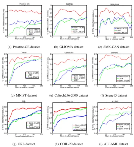
2)Results for the Semi-supervised Case (Semi-JHLSR): The classiÞcation
ac-440
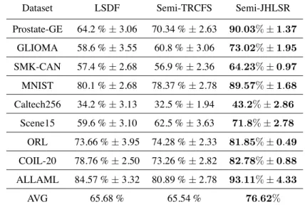
curacies for the different feature subsets obtained using semi-supervised learning are shown in Fig.5 and Table. 4. Again, we observe that our proposed method Semi-JHLSR outperforms the alternatives. The aggregated SVM classiÞcation accuracy in Table. 4 also clearly shows that the proposed method outperforms each of the competing semi-supervised methods for all datasets studied, and the improvement is in the range from
445
4.02%to 25.83%. Based on these results, we observe that simultaneously preserving both the sample similarity and the local geometric structure of data is necessary in identifying discriminative features.
Table 4: Study of Semi-supervised cases: aggregated SVM classiÞcation accuracy (MEAN±STD). The last row shows the averaged classiÞcation accuracy of all the algorithms over the 9 datasets.
Dataset LSDF Semi-TRCFS Semi-JHLSR Prostate-GE 64.2 %±3.06 70.34 %±2.63 90.03%±1.37 GLIOMA 58.6 %±3.55 60.8 %±3.06 73.02%±1.95 SMK-CAN 57.4 %±2.68 56.9 %±2.36 64.23%±0.97 MNIST 80.1 %±2.68 78.37 %±2.78 89.57%±1.68 Caltech256 34.2 %±3.13 32.5 %±1.94 43.2%±2.86 Scene15 59.6 %±3.10 62.5 %±3.63 71.8%±2.78 ORL 73.66 %±3.95 74.28 %±2.33 81.85%±0.49 COIL-20 78.76 %±2.50 73.26 %±2.82 82.78%±0.88 ALLAML 84.57 %±3.32 80.89 %±2.78 93.11%±4.33 AVG 65.68 % 65.54 % 76.62%
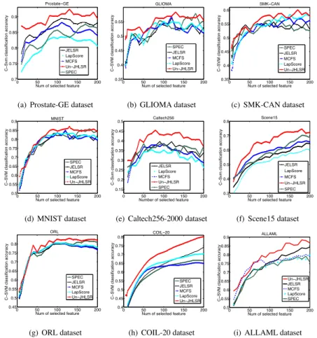
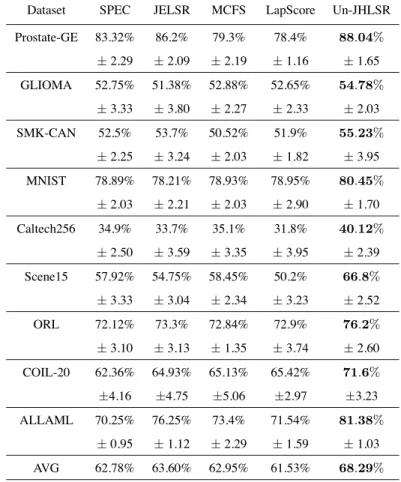
3)Results for the Unsupervised Case (Un-JHLSR): From Fig.6, the proposed method Un-JHLSR still maintains the best classiÞcation accuracy on each of the 9
450
benchmark data sets. The aggregated SVM classiÞcation accuracy of different algo-rithms on each data set is shown in Table. 5. From the results, we draw the following two observations: (1) Firstly, the joint manifold characterization and feature selection methods outperform the methods which separate these two procedures, i.e., Un-JHLSR and JELSR are superior to MCFS and LapScore in terms of accuracy in most cases.
455
(2) Secondly, the proposed method Un-JHLSR shows a signiÞcant improvement over the graph based method JELSR. There are three reasons for this improvement in per-formance. First, The local structure in JELSR is based on ak-nearest neighbor graph, while UN-JHLSR leans a hypergraph. Compared with graph regularization, hyper-graph regularization imposes a much stronger constraint on the data samples. Instead
460
of approximating them in terms of pairwise interactions which can lead to a substantial loss of information, the hypergraph representation is effective in capturing the high-order relations among samples. Thus the structural information latent in the data can be effectively preserved. Second, JELSR iteratively performs spectral embedding for
0 50 100 150 200 0.7 0.75 0.8 0.85 0.9 Prostate−GE C − Svm cl a ssi fi ca ti o n a ccu ra cy
Num of selected feature JELSR LapScore MCFS Un−JHLSR SPEC
(a) Prostate-GE dataset
0 50 100 150 200 0.35 0.4 0.45 0.5 0.55 GLIOMA C − SVM cl a ssi fi ca ti o n a ccu ra cy
Num of selected feature SPEC JELSR MCFS LapScore Un−JHLSR (b) GLIOMA dataset 0 50 100 150 200 0.35 0.4 0.45 0.5 0.55 0.6 SMK−CAN C − SVM cl a ssi fi ca ti o n a ccu ra cy
Num of selected feature SPEC JELSR MCFS LapScore Un−JHLSR (c) SMK-CAN dataset 0 50 100 150 200 0.5 0.55 0.6 0.65 0.7 0.75 0.8 0.85 0.9 MNIST C − SVM cl a ssi fi ca ti o n a ccu ra cy
Num of selected feature SPEC JELSR MCFS LapScore Un−JHLSR (d) MNIST dataset 0 50 100 150 200 0.15 0.2 0.25 0.3 0.35 0.4 0.45 0.5 Caltech256 C − Svm cl a ssi fi ca ti o n a ccu ra cy
Number of selected feature JELSR LapScore MCFS Un−JHLSR SPEC
(e) Caltech256-2000 dataset
0 50 100 150 200 0.3 0.4 0.5 0.6 0.7 0.8 Scene15 C − Svm cl a ssi fi ca ti o n a ccu ra cy
Num of selected feature JELSR LapScore MCFS Un−JHLSR SPEC (f) Scene15 dataset 0 50 100 150 200 0.45 0.5 0.55 0.6 0.65 0.7 0.75 0.8 ORL C − SVM cl a ssi fi ca ti o n a ccu ra cy
Num of selected feature SPEC JELSR MCFS LapScore Un−JHLSR (g) ORL dataset 0 50 100 150 200 0.4 0.45 0.5 0.55 0.6 0.65 0.7 0.75 0.8 COIL−20 C − SVM cl a ssi fi ca ti o n a ccu ra cy
Num of selected feature SPEC JELSR MCFS LapScore Un−JHLSR (h) COIL-20 dataset 0 50 100 150 200 0.5 0.55 0.6 0.65 0.7 0.75 0.8 0.85 0.9
Num of selected feature
C − SVM cl a ssi fi ca ti o n a ccu ra cy ALLAML Un−JHLSR JELSR MCFS LapScore SPEC
(i) ALLAML dataset
Figure 6: Accuracy rate vs. the number of selected features on 9 benchmark datasets by unsupervised learning.
clustering and sparse spectral regression for feature selection. However, the local
struc-465
ture itself (i.e. the Laplacian matrix) is not changed during iterations of the algorithm. Our proposed method JHLSR can adaptively improve the local structure by learning the weights of hypergraph. Third, unlike JELSR which only incorporating the local manifold structure, our proposed method JHLSR integrates the merits of local mani-fold structure and global discriminative sample similarity. Thus, it performs better than
470
the traditional methods.
Taken together, the above experimental results for the supervised, unsupervised, and semi-supervised feature selection modalities demonstrate the effectiveness and
ef-Table 5: Study of Unsupervised cases: aggregated SVM classiÞcation accuracy (MEAN±STD). The last row shows the averaged classiÞcation accuracy of all the algorithms over the 9 datasets.
Dataset SPEC JELSR MCFS LapScore Un-JHLSR Prostate-GE 83.32% 86.2% 79.3% 78.4% 88 .04% ±2.29 ±2.09 ±2.19 ±1.16 ±1.65 GLIOMA 52.75% 51.38% 52.88% 52.65% 54 .78% ±3.33 ±3.80 ±2.27 ±2.33 ±2.03 SMK-CAN 52.5% 53.7% 50.52% 51.9% 55 .23% ±2.25 ±3.24 ±2.03 ±1.82 ±3.95 MNIST 78.89% 78.21% 78.93% 78.95% 80 .45% ±2.03 ±2.21 ±2.03 ±2.90 ±1.70 Caltech256 34.9% 33.7% 35.1% 31.8% 40 .12% ±2.50 ±3.59 ±3.35 ±3.95 ±2.39 Scene15 57.92% 54.75% 58.45% 50.2% 66 .8% ±3.33 ±3.04 ±2.34 ±3.23 ±2.52 ORL 72.12% 73.3% 72.84% 72.9% 76 .2% ±3.10 ±3.13 ±1.35 ±3.74 ±2.60 COIL-20 62.36% 64.93% 65.13% 65.42% 71 .6% ±4.16 ±4.75 ±5.06 ±2.97 ±3.23 ALLAML 70.25% 76.25% 73.4% 71.54% 81 .38% ±0.95 ±1.12 ±2.29 ±1.59 ±1.03 AVG 62.78% 63.60% 62.95% 61.53% 68 .29%
Þciency of the proposed JHLSR framework.
7.4. Convergence Results 475
In this section, we provide some numerical results to illustrate the convergence behavior of our algorithm JHLSR. Two datasets, i.e., COIL-20 and GLIOMA, are em-ployed. SinceS is used for feature selection, we would like to measure the variance between two sequentialSusing the following metric:
0 2 4 6 8 10 12 14 16 18 20 0 2 4 6 8 10 12
14 Divergence on COIL−20 in supervised case
(a) COIL-20: Supervised case
0 2 4 6 8 10 12 14 16 18 20 0 2 4 6 8 10 12 14 16
18 Divergence on COIL−20 in Semi−supervised case
(b) COIL-20: Semi-supervised case 0 2 4 6 8 10 12 14 16 18 20 0 2 4 6 8 10 12 14 16
18 Divergence on COIL−20 in Un−supervised case
(c) COIL-20: Un-supervised case 0 2 4 6 8 10 12 14 16 18 20 0 2 4 6 8
10 Divergence on GLIOMA in Supervised case
(d) GLIOMA: Supervised case
0 2 4 6 8 10 12 14 16 18 20 0 1 2 3 4 5 6 7
8 Divergence on GLIOMA in Semi−supervised case
(e) GLIOMA: Semi-supervised case 0 2 4 6 8 10 12 14 16 18 20 0 2 4 6 8 10
12 Divergence on GLIOMA in Un−supervised case
(f) GLIOMA: Un-supervised case
Figure 7: Convergence behavior of JHLSR. There are mainly 20 iterations.x-axis represents the number of iterations andy-axis represents the divergence between two sonsecutiveSmeasure by Eq.29. As observed, JHLSR always converge within 4 iterations.
As seen from Fig.7, the divergence between two consecutiveS converges to zero, which means that the Þnal results will not be changed drastically. Convergence is fast, requiring less than 4 iterations.
7.5. Effect of Adaptive Structure Learning by Hypergraph
To further illustrate the effectiveness of JHLSR in preserving the local manifold
480
structure of the data, we compare JHLSR with regular hypergraph learning (HYPER) [21] (i.e. with no learning of the hyperedge weights) and a graph based version of the proposed algorithm (referred to as GRAPH). The main experimental results are presented in Fig.8 and a few interesting observations can be made. First, JHLSR con-sistently outperforms HYPER and GRAPH on all the datasets studied. The main
rea-485
son is that JHLSR can represent diverse relations among data samples, and adaptively improve the local structure from the results of hypergraph learning. Second, JHLSR consistently performs better than the conventional hypergraph learning algorithm (i.e. HYPER), and this result suggests that the simultaneous learning of hyperedge weights and feature selection is a better strategy. Third, for the supervised case, there are few
490
differences among the three methods, since the label information is more crucial than modeling the local manifold structure of data for the subsequent classiÞcation task.
0 50 100 150 200 0.2 0.25 0.3 0.35 0.4 0.45 Caltech256 C − SVM cl assi fi cat ion accuracy
Num of selected feature Sup−JHLSR GRAPH
HYPER
(a) Caltech256: Supervised case 0 50 100 150 200 0.2 0.25 0.3 0.35 0.4 0.45 0.5 Caltech256 C − SVM cl assi fi cat ion accuracy
Num of selected feature Semi−JHLSR HYPER GRAPH (b) Caltech256: Semi-supervised case 0 50 100 150 200 0.15 0.2 0.25 0.3 0.35 0.4 0.45 0.5 Caltech256 C − Svm cl assi fi ca ti on accuracy
Number of selected feature Un−JHLSR GRAPH HYPER (c) Caltech256: Un-supervised case 0 50 100 150 200 0.4 0.45 0.5 0.55 0.6 0.65 0.7 0.75 0.8 C − SVM cl assi fi cat ion accuracy
Num of selected feature Scene15 sup−JHLSR GRAPH HYPER (d) Scene15: Supervised case 0 50 100 150 200 0.4 0.45 0.5 0.55 0.6 0.65 0.7 0.75 0.8 SVMs cl assi fi cat ion accuracy
Num of selected feature Scene15
Semi−JHLSR GRAPH HYPER
(e) Scene15: Semi-supervised case 0 50 100 150 200 0.3 0.4 0.5 0.6 0.7 C − SVM cl assi fi cat ion accuracy
Num of selected feature Scene15 Un−JHLSR GRAPH HYPER (f) Scene15: Un-supervised case 0 50 100 150 200 0.4 0.45 0.5 0.55 0.6 0.65 0.7 0.75 0.8 C − SVM cl a ssi fi ca ti o n a ccuracy
Num of selected feature SMK−CAN sup−JHLSR GRAPH HYPER (g) SMK-CAN: Supervised case 0 50 100 150 200 0.4 0.45 0.5 0.55 0.6 0.65 0.7 C − SVM cl a ssi fi ca ti o n a ccuracy
Num of selected feature SMK−CAN Semi−JHLSR GRAPH HYPER (h) SMK-CAN: Semi-supervised case 0 50 100 150 200 0.25 0.3 0.35 0.4 0.45 0.5 0.55 0.6 C − SVM cl a ssi fi ca ti o n a ccuracy
Num of selected feature SMK−CAN
Un−JHLSR GRAPH
HYPER
(i) SMK-CAN: Un-supervised case
Figure 8: Accuracy rate vs. the number of selected features on three benchmark datasets by different methods (JHLSR,HYPER,GRAPH).
However, in the semi-supervised and unsupervised cases, JHLSR gains a signiÞcant improvement over HYPER and GRAPH. This is because when the labeled data are scarce, feature selection aims to select the features that well maintain the underlying
lo-495
cal manifold structure. In this case, the local structure itself (i.e. the Laplacian matrix) in HYPER is not changed during iterations of the algorithm. JHLSR can adaptively improve the local manifold structure by updating the hyperedge weights.