Discussion Papers in Economics
Discussion Paper No. 11/03
Identifiability and estimation
of the sign of a covariate effect
in the competing risks model
S.M.S. Lo and R.A. Wilke
April 2011
Identifiability and estimation of the sign of a covariate effect
in the competing risks model.
∗
Simon M.S. Lo
†Ralf A. Wilke
‡April 2011
∗We thank Lutz D¨umbgen for helpful discussions and the participants at numerous seminars for their comments.
Wilke is supported by the Economic and Social Research Council through theBounds for Competing Risks Duration Models using Administrative Unemployment Duration Data(RES-061-25-0059) grant.
†Lingnan University, Rm 218, Ho Sin Hang Building, Lingnan University, Hong Kong, E–mail:
‡University of Nottingham, School of Economics, University Park, Nottingham NG7 2RD, United Kingdom,
Abstract
It is well known that the competing risks model is identified if the dependence structure between risks (the copula function) is known or assumed. Special cases include indepen-dence of risks or independent censoring. If the copula function is not specified, parameters of interest are only set identified. As these sets are often wide in applications, it is difficult to obtain informative results. In this paper we strike a balance between imposing too much and too little structure. By establishing a general link between observable changes in sub-distributions (cumulative incidence curves) and the sign of changes in marginal sub-distributions (the causal treatment effect) we are able to show the identifiability of the latter if the copula function is independent of the varying covariate. This has two important implications: First, it is possible to obtain informative results even if the copula function is mainly unspecified or unknown. Second, the sign of the covariate effect tends to be invariant with respect to the chosen dependence structure. Our method is computationally very simple and our sim-ulations suggest that it identifies and consistently estimates the sign of the treatment effect for large sets of duration times. An application to unemployment duration data illustrates the usefulness of our method for empirical research.
Keywords: dependent censoring, nonparametric estimation, bootstrap JEL: C14, C24, C41
1
Introduction
The non-identifiability of the competing risks model (Cox, 1962; Tsiatis, 1975) implies that data alone is only partly informative for the identification of the parameters of interest. If we are, for example, interested in the marginal distribution of a latent competing variable, this functional can only be bounded (Peterson, 1976). See also Manski (2003) for partially identified probability distributions. Honor´e and Lleras-Muney (2006) consider the accelerated failure time model and obtain tighter bounds on the marginal effect from discrete covariates. Point identification can be achieved by making assumptions on the marginal distributions and the dependence structure between the competing risks (Abbring and van den Berg, 2003) or by fully specifying a the dependence structure (a copula function) between the competing risks (Zheng and Klein, 1995). By performing a sensitivity analysis, Lo and Wilke (2010) observe that the sign of a covariate effect
-thecausal treatment effect - is often the same for any assumed copula function while the magnitude of the effect varies considerably. Basing on this observation we take a different route in this paper by focusing on the identifiability of the sign of a covariate effect rather than its magnitude. Indeed, we can show that it is identifiable by exploiting variation in the cumulative incidence curves (CIC) and the survival function of the observed failure time under a mild condition. Our simulations and illustrations with data suggest that our identification approach provides substantially more informative results than the Peterson bounds. Our method is very simple and general as it is fast to compute and it works with existing non-, semi- and parametric estimators for the CICs (e.g. Jeong and Fine, 2007, and Peng and Fine, 2009). Although our approach is less informative than point estimates, we claim that it still is very informative for research in various disciplines such as biometrics, econometrics and social sciences. We therefore conceive our novel approach as a useful tool for a wide research community.
The structure of this paper is as follows: the next section introduces the model and presents our main identification results. Section 3 suggests nonparametric estimation and inference procedures. Section 4 presents simulation results. Section 5 illustrates our method by estimating the effect of various covariates on the job finding probability for unemployed individuals in Germany.
2
Identifiability
We first consider a model with two latent competing random variables T1 and T2 ∈ IT ⊂ R+. A model with more than two competing risks is considered in Section 2.2. T1 and T2 are times
to failure or times to the events 1 and 2 respectively. While T1 and T2 are not observable,
T = min(T1, T2) and δ = argminjTj are observed. There is one observable binary covariate x
which takes valuesx=x0 (control group) andx=x1 (treatment group). Data on (T, δ, x) enable
the identifiability of the unknown cumulative incidence curves Qj(t;x) = Pr(T ≤ t, δ = j| x),
the unknown cause-specific crude hazard functions λj(t;x) = lim∆→0Pr(t ≤ T ≤ t + ∆, δ =
j|T ≥ t, x)/∆ for risk j = 1,2 and the unknown survival function S(t;x) = Pr(T > t| x) of
T = min(T1, T2) for all t. The marginal distribution functions Fj(t;x) = Pr(Tj ≤ t| x) and the
marginal survival functions Sj(t;x) = 1−Fj(t;x) are also unknown for all j and t but they are
not identifiable from data alone (Cox, 1962; Tsiatis, 1975).
all j.
Let be S−1 the inverse of the functional S. We denote ∆
xFj(t) = Fj(t;x1)−Fj(t;x0) as the covariate or treatment effect onFj(t;x0) and its direction bysign|∆xFj(t)|. The operatorsign|w|
equals to the sign of the variablew. It is +1, 0 or -1 ifwis positive, zero or negative respectively.
In our model ∆xFj(t) is unknown and not identified. However, in the following we show that
sign|∆xFj(t)| can be identified from the CICs and the survival function for some duration time
under a very mild condition. Note that in contrast to popular semiparametric models such as the proportional hazard model there is no restriction on the nature of the treatment effect acting on the duration time as the sign of ∆xFj(t) can vary with t.
An integral part of the competing risks model is the dependence structure between the risks which is determined by the survival copula C(s1, s2;x) = Pr(S1 ≤s1, S2 ≤s2;x). The competing risks model is fully characterised by
Q1(t;x) = ∫ζ21(s1;x) 0 ∫1 S1(t;x)C ′′(s 1, s2;x) ds1 ds2; S(t;x) = C{S1(t;x), S2(t;x);x}, (1)
whereζ21(s1;x) =S2{S1−1(s1;x);x}is a unique link function that defines the relationship between
S1(t;x) andS2(t;x) for alltandx(Lemma A1 of Zheng and Klein, 1995). For more details see also
Lo and Wilke (2010). The probability density function of the copula is denoted byC′′(s1, s2;x) =
∂2C(s
1, s2;x)/∂s1∂s2. Model (1) implies that S1(t;x) and S2(t;x) are determined jointly by the copula functionS(t;x) = C{S1(t;x), S2(t;x);x}and the link functionS2(t;x) = ζ21{S1(t;x);x}as
Qj(t;x) and S(t;x) are directly identified from the data. When the copula function is known, the
link function is fixed byQ1(t;x). Then the two unknownsS1(t;x) andS2(t;x) can be determined by solving the two equations for allt.
In this paper we consider a model with an unknown copula functionC(s1, s2;x). For this reason
ζ21 and Fj for all j are not identified. Without imposing additional assumptions, the treatment
effect can only be bounded by using the Peterson bounds for the marginal distributions:
∆xQj(t)−Qi(t;x0) ≤∆xFj(t)≤ ∆xQj(t) +Qi(t;x1) (2) with ∆xQj(t) = Qj(t;x1)−Qj(t;x0) for j = 1,2 and j ̸=i. We denote IPj as the nonparametric
identification set for sign|∆xFj(t)|. IPj consists of all t for which ∆xQj(t)−Qi(t;x0) > 0 or ∆xQj(t) +Qi(t;x1)<0 or the two former being equal to zero. As the Peterson bounds are often
wide,IPj is likely small and no informative result can be obtained in an application. In the following
we show that it is possible to obtain a considerably larger, although different, identification set by imposing a restriction on the unknown copula function.
Assumption 2 C(s1, s2;x1) = C(s1, s2;x0) = C(s1, s2).
Despite being difficult to test in applications, most popular parametric, semi-, and non-parametric duration models make stronger assumptions on the dependence structure which imply Assumption 2. This includes the Kaplan-Meier estimator, the accelerated failure time model and the (mixed) proportional hazard model. For more details see Bond and Shaw (2006). In their paper they derive bounds for covariate-time transformations under a condition which implies Assumption 2. Although Assumption 2 limits the covariate effect to Fj(t;x) for all j, ζ21(s1;x) and S(t;x) still
change withx. Assumption 2 is a crucial condition for our approach to identification, as it builds up observable linkages between the observable changes in the CICs and the unobserved changes in the marginal distributions. It can be seen from (1) that, when the integrandC′′ is unaffected by the treatment, the direction of the covariate effect onQ1(t;x) and F1(t;x) can be analyzed by the
changes in the size of the two domains in the integration function ofQ1(t;x). For the purpose of illustration let us consider a special case where the treatment acts positively onF1(t) while keeping
F2(t) constant for all t. In this case,S1(t;x1)< S1(t;x0) for all t, and ζ21(s1;x1)> ζ21(s1;x0) for alls1. Thus, Q1(t;x1) = ∫ ζ21(s1;x1) 0 ∫ 1 S1(t;x1) C′′ ds1 ds2 > ∫ ζ21(s1;x0) 0 ∫ 1 S1(t;x1) C′′ ds1 ds2 > ∫ ζ21(s1;x0) 0 ∫ 1 S1(t;x0) C′′ ds1 ds2 =Q1(t;x0).
Therefore,Q1(t;x) increases withF1(t;x) for allt. This special case illustrates that there is a link
between the direction of the covariate effect on Fj and the sign of the effect onQj.
To fully develop this observation into a general result, we exploit the fact that S1(t;x) and
S2(t;x) are jointly determined by the copula function and the link function. We consider an analytical 2-part decomposition of the change in the marginal distributions, where we isolate two effects. The first part is the counterfactual movement of the marginal distributions due to the change in the link function fromζ21(s1;x0) toζ21(s1;x1) while keeping the copula function constant
that S1 and S2 become the solutions of (i) C{S1(tc;x1), S2(tc;x1)}=C{S1(t;x0), S2(t;x0)} or
S(tc;x1) = S(t;x0) (3)
and (ii)S2(tc;x1) = ζ21{S1(tc;x1);x1}. This is denoted as the copula effect.
Definition 1 The copula effect of a covariate change from x0 to x1 on the marginal distribution
in model (1) is defined by ∆c
xFj(t) = Fj(tc;x1)−Fj(t;x0), with tc satisfying condition (3). The difference betweentcandthas an interpretation of a quantile treatment effect at theS(t;x
0 )-quantile. tc and t are generally different if the link function ζ
21(s1;x) changes in response to a covariate change, except when t=tc= 0 at S(t;x
0) =S(tc;x1) = 1.
The second part of the decomposition characterises the changes in the marginal distributions to [S1(t, x1), S2(t, x1)] which are due to the change from S(t;x0) toS(t;x1) while keeping the link function unchanged. S1 and S2 become solutions to (i) C{S1(t;x1), S2(t;x1)} =S(t;x1) and (ii)
S2(t;x1) =ζ21{S1(t;x1);x1}. We denote this as the marginal distribution effect.
Definition 2 The marginal distribution effect of a covariate change fromx0 tox1 on the marginal
distributionFj(t, x0) in model (1) is defined by ∆mxFj(t) =Fj(t;x1)−Fj(tc;x1), with tc satisfying
condition (3).
A graphical presentation of ∆m
xFj(t) and ∆cxFj(t) is given in the supplemental material. We
obtain the following useful results.
Lemma 1 Under Assumptions 1 and 2 we have for all t∈IT in Model (1):
1. ∆cxFj(t) and ∆mxFj(t) are unique for all j.
2.
∆xFj(t) = ∆cxFj(t) + ∆mxFj(t) for all j. (4)
3. sign|∆c
xFj(t)| and sign|∆mxFj(t)| determine the sign of ∆xFj(t) for at least one j.
The uniqueness follows from the uniqueness oftc. The decomposition in (4) follows directly from
Definitions 1 and 2. For more details on the proof see the Appendix. As a next step we define observable analogues of the marginal distribution effect and the copula effect.
Definition 3 We define ∆cxQj(t) = Qj(tc;x1)−Qj(t;x0)as the copula effect on the CIC for risk
j = 1,2 for all t in model (1), with tc satisfying the condition (3).
Definition 4 We define ∆mxQj(t) = Qj(t;x1)−Qj(tc;x1) as the marginal distribution effect on
the CIC for risk j = 1,2 for all t in model (1), with tc satisfying condition (3).
A graphical illustration of ∆m
xQj(t) and ∆cxQj(t) is also given in the supplemental material. The
following two lemmas establish systematic relationships between the unobserved sign|∆c xFj(t)|
and sign|∆m
xFj(t)| and the observable analogues based on the CICs.
Lemma 2 In model (1) under Assumptions 1 and 2, we have for j = 1,2 and for all t
sign|∆mxFj(t)| = sign|∆mxQj(t)|. (5)
Lemma 2 can be proved by using Definitions 2 and 4. Fj(t;x) and Qj(t;x) are both strictly
increasing functions int, and thus sign|∆m
xFj(t;x)| equals sign|∆xmQj(t;x)|for any tc and t. As
the equivalent result for the copula effect does not hold for allt, we consider a restricted set only.
Definition 5 Let {´tk} for k = 0,1,2, . . . be a finite sequence of t ∈ IT such that ∆cxQj(´tk) = 0
with´t0 = 0. Let {`tk} for k= 1,2, . . . be a finite sequence oft ∈IT such that|∆cxQj(t)| has its first
local maximum in the interval (´tk−1,´tk]. Moreover, IIj = ∪
k≥0[´tk,t`k+1]⊂IT.
IIj is observable since ´tk and `tk are observed for allk. The following result suggests that IIj is the
identification set for the sign of the copula effect on the marginal distributions for riskj.
Lemma 3 In model (1) under Assumptions 1 and 2, we have for j = 1,2 and for all t ∈IIj
sign|∆cxFj(t)| = sign|∆cxQj(t)|. (6)
The proof of Lemma 3 can be found in the Appendix. The intuition behind Lemma 3 can be illustrated by a special case where the link function ζ21(s1, x) is a monotone function in x. We have for alls1 either (i)ζ21(s1, x1)≤ζ21(s1, x0) or (ii)ζ21(s1, x1)≥ζ21(s1, x0). Under Assumption 2, case (i) implies that the copula effect on F1(t) is negative and it is positive on F2(t) for all t.
See also Lemma A3 in the Appendix for a formal derivation. This implies S1(tc;x1) < S1(t;x0) and S2(tc;x1)> S2(t;x0) with C{S1(tc;x1), S2(tc;x1)}=C{S1(t;x1), S2(t;x1)}. It follows that
Q1(tc;x1) = ∫ ζ21(s1;x1) 0 ∫ 1 S1(tc;x1) C′′ ds1 ds2 < ∫ ζ21(s1;x0) 0 ∫ 1 S1(tc;x1) C′′ ds1 ds2 < ∫ ζ21(s1;x0) 0 ∫ 1 S1(t;x0) C′′ ds1 ds2 =Q1(t;x0).
Analogous reasoning can be applied to case (ii). And thus the sign of the copula effect on Qj(t)
and Fj(t) are the same for all t. In the general case where ζ21(s1, x) is not a monotone function,
say, ζ21(s1, x1) and ζ21(s1, x0) cross each other at a sequence of duration time {t˙k} ∈ IT for
k= 0,1,2, . . ., the relationship between the sign of|∆c
xQj(t)|and|∆cxFj(t)|can only be established
when{t˙k} is known. But as ζ21(s1, x) is unidentified,{t˙k} can only be bounded. We show in the
Appendix that ˙t is bounded by the observed interval [`tk,´tk] for all k ≥ 0. The sign of |∆cxQj(t)|
can therefore be identified for the observable sequence of sets [´tk,`tk+1] for all k ≥0 which is IIj.
According to Lemmas 1, 2 and 3,sign|∆xFj(t)|is determined bysign|∆mxQj(t)|andsign|∆cxQj(t)|
for all t ∈ IIj. Let us denote ∆xQj(t) = [∆cxQj(t),∆mxQj(t)]′. ∆xQj(t)0 means that both of
∆c
xQj(t) and ∆mxQj(t) are nonnegative but that at least one is non-zero. ∆xQj(t)0 is defined
analogously. Moreover, letIDj ⊂ IT consist of all t such that ∆cxQj(t)×∆mxQj(t)≥ 0. ThenIDj
consists of all t such that ∆m
xQj(t) and ∆cxQj(t) do not have an opposite sign. We are now able
to state our main identification result.
Proposition 1 Under Assumptions 1 and 2, the sign of the treatment effect in model (1) is
identified for allt ∈IIj ∩ IDj. We have sign|∆xFj(t)| = +1 if ∆xQj(t)0; 0 if ∆xQj(t) =0; −1 if ∆xQj(t)0. (7)
Moreover, it is identified for at least one risk j = 1,2 for all t ∈IIj.
Proposition 1 follows directly from all previous results. It suggest thatsign|∆xFj(t)| is identified
fort ∈IIj if ∆mxQj(t) and ∆mxQj(t) do not the have opposite sign.
2.1
Increasing the identification set
Proposition 1 suggests that the direction of the treatment effect is unidentified if ∆c
xQj(t) and
∆m
identification set. As it does not require any additional assumption it should always be performed. Rather than the treatment effect, we consider the reversed treatment effect
∆−xFj(t) =Fj(t;x0)−Fj(t;x1) = −∆xFj(t). (8)
The reversed treatment effect is the change inFj(t;x) from x1 tox0 and, thus, has the opposite sign than ∆xFj(t). It is obvious that Proposition 1 also holds for the reversed treatment effect by
exchanging the notationx1 andx0. We denote this property as independence of the decomposition
route. Let IIj(x) ∩
IDj(x) and IIj(−x) ∩
IDj(−x) be the identification sets for sign|∆xFj(t)| and
sign|∆−xFj(t)|respectively. We obtain the following useful result. Corollary 1 IIj(x)
∩
IDj(x)̸=IIj(−x) ∩
IDj(−x).
We prove Corollary 1 by showing that for some t the sign of the treatment effect is unidentified, while the sign of the reversed treatment effect is identified. The proof is given in the Appendix.
Corollary 1 suggests that it is always better to compute both decomposition routes and take the union of the two identification sets. Since the underlying identification approach of the Peterson bounds in (2) and our method are also different, it is advisable to determine the identification sets for all approaches and take the union of all sets for each risk
Qj =IPj ∪ { IIj(x) ∩ IDj(x) } ∪ { IIj(−x) ∩ IDj(−x) } ⊂IT.
For all t ∈ Qj\IPj we can also tighten the bounds for the magnitude. If the sign of the effect
is negative (positive) the lower (upper) bound for the magnitude is the lower (upper) Peterson bound and the upper (lower) bound is 0.
2.2
Identifiability in a multi-risks model
In this section we extend the identification result of the previous section to a model with a finite number of risksJ >2. The observed failure time becomes T = min(T1, . . . , TJ) and the indicator
function isδ= argminjTj. Model (1) becomes
Qj(t;x) = ∫ζJ j(sj;x) 0 . . . , ∫ζj+1j(sj;x) 0 ∫1 Sj(t;x) ∫ζj−1j(sj;x) 0 . . . ∫ζ1j(sj;x) 0 ∂JC(s 1,...,sJ;x) ∂s1...,∂sJ ds1. . . dsJ; S(t;x) = CJ(s 1, . . . , sj, . . . , . . . , sJ;x). (9)
The J-survival copula is
CJ(s1, . . . , sJ;x) = Pr{S1(T1;x)≤s1, . . . , SJ(TJ;x)≤sJ;x}. (10)
To carry over the identification results of the last section with J = 2, we follow the risk pooling approach by Lo and Wilke (2010). Suppose that we want to identify the sign of the treatment effect on risk j. By conceptually pooling all other risks into a single risk, we generate an unobserved new variableT−j = min(T1, . . . , Tj−1, Tj+1, . . . , TJ). This is then a two risks model with a 2-copula
C2(sj, s−j;x) = Pr{Sj(Tj;x)≤sj, S−j(T−j;x)≤s−j;x}. (11)
The unknown marginal survival function for the pooled variableT−j isS−j(t;x) = Pr(T−j > t;x).
The observed failure time is unaffected asT = min(Tj, T−j), and the indicator function is modified
as δj =j if the original δ =j and δj =−j if δ ̸= j. For any J-copula in (10), the existence of a
2-copula in (11) is guaranteed under the following assumption (Nelsen, 2006).
Assumption 3 In the competing risks model defined by (9) the survival copula belongs to the
Archimedean class.
In this case the multi-risk model can be reduced into a two risks model as (1):
Qj(t;x) = ∫ζ−j,j(sj;x) 0 ∫1 Sj(t;x)C ′′ ds j. . . ds−j; S(t;x) = C2{S j(t, x);S−j(t;x);x}, (12)
with s−j = ζ−j,j(sj;x) denotes the link function between Sj(t;x) and S−j(t;x). For more details
see Lo and Wilke (2010). Our identification approach for the two risks model can therefore be subsequently applied to (12) for j = 1, . . . , J, where the order of application does not matter.
Note, however, that only one risk is of interest in the pooled risks model as the pooled risks are generally uninformative.
3
Estimation
For simplicity we outline the estimation procedure for a two risks model. Suppose we have for x0 and x1 two finite samples of observations of T = min{T1, T2} with latent failure time identically and independently distributed as T1 ∼ F1(T1;x) and T2 ∼ F2(T2;x), δ = argminjTj
and only (T, δ, x) is observed. We suggest an estimation procedure which involves several stages. First, we estimate Qj(t;x) and S(t;x) with common nonparametric estimators (Kalbfleish and
Prentice, 2002), although any existing consistent (non-)parametric estimator could be used. These estimators are then plugged into the equations of the previous section to obtain their sample analogues. In what follows we list all steps of the estimation procedure:
1. Define an equally spaced grid{t0, t1, . . . , tM}.
2. Estimate ˆQj(t;xk) and ˆS(t;xk) for j, k = 0,1 nonparametrically at all t in{t0, t1, . . . , tM}.
3. Determinetcby solving the sample analogue of equation (3) for alltin{t
0, t1, . . . , tM}. Since
the estimated survival curves are step functions, we assume left continuity of ˆS(t;xk). Thus
for any value of ti, tj, tj+1 on the time grid such that ˆS(tj, x1)>Sˆ(ti, x0)>Sˆ(tj+1, x1). The solution to equation (3) is tc
i =tj+1.
4. Compute ∆m
xQˆj(t) by pluggingtcinto ˆQj(t;x) according to Definition 4, for alltin{t0, t1, . . . , tM}.
5. Compute ∆c
xQˆj(t) by pluggingtcinto ˆQj(t;x) according to Definition 3, for alltin{t0, t1, . . . , tM}.
6. For all j estimate IIj from the sequences {t´k} and {`tk} according to Definition 5 by using
ˆ
Qc
j(t;x). Estimate IDj by using sign|∆mxQˆj(t)| and sign|∆cxQˆj(t)| for all j.
7. The sign of the time-specific treatment effect is then determined by the sample analogues of Proposition 1.
This procedure is applicable to both directions of the decomposition ∆x and ∆−x, which results in
different identification sets for each risk. Before we consider large sample properties and inference, we briefly outline two modifications to improve the finite sample performance:
• Sampling variation in ˆQj(t) also implies some random variation in ∆cxQˆj(t). For this reason,
the estimated sequence {`tk}has also some random variation. In particular since ∆cxQˆj(t) is
not smooth and has some peaks created by the noise in the data, the estimated first local extreme value between {´tk}x and{t´k+1}x is likely to occur before the actual value of {`tk+1}. This implies that the estimated{`tk+1}as well as the size of the identification region are often downward biased in small samples. We suggest two alternative procedures to overcome this issue:
– Employ a smoothing technique for ˆQj(t) in step 5 to eliminate small peaks in ∆cxQˆj(t).
Although it can eliminate peaks due to random sampling, it can also eliminate the true extreme values if the chosen degree of smoothing is too large. As with any smoothing technique there is some arbitrariness involved and it is difficult to determine the optimal degree of smoothing.
– Impose an additional assumption that there are no multiple extreme values of ∆cxQˆj(t)
between {´tk} and {t´k+1}. In this case, we recommend in step 6 the use of thet corre-sponding to the estimated global extreme value between{t´k}and{´tk+1}as an estimator for the sequence{`tk}. This method produces good results if the true copula effect does
not have multiple local extreme values. Otherwise, the estimated{`tk}is upward biased.
3.1
Consistency
Proposition 2 Assume that Sˆ −→p S (convergence in probability) and Qˆj
p
−→ Q for all j or assume almost sure convergence. Then under Assumptions 1, 2 and 3 we have for model (12)
sign|∆xFˆj(t)| = +1 if ∆xQˆj(t)0; 0 if ∆xQˆj(t) =0; −1 if ∆xQˆj(t)0. (13)
converges in probability (or almost surely) to sign|∆xFj(t)| for all j and all t ∈IIj ∩
IDj.
Whether we have weak or strong consistency depends on the choice of the estimators for ˆS(t, x) and ˆQj(t, x). The proof is a straightforward application of the continuous mapping theorem (Van
der Vaart, 1998, Theorem, 18.11) provided thatS(t, x) and Qj(t, x) are continuous for all j.
Proof: For simplicity we only show weak consistency, i.e. sign|∆xFˆj(t)| p
−→sign|∆xFj(t)|. First
note that provided ˆS(t, x)−→p S(t, x) andS(t, x) is continuous, we have ˆS−1( ˆS(t, x
0), x1) = ˆtc p −→
tc. Then, since ˆQj(t, x) p
−→Qj(t, x),Qj(t, x) is continuous, and since ˆtc p −→ tc, we have ∆cxQˆj(t) p −→ ∆c xQj(t) and ∆mxQˆj(t) p −→ ∆m
xQj(t) for all j. Then all stochastic components in the right
3.2
Inference
Under the assumption that observations are independent, we can perform a statistical test for the sign of the treatment effect ∆xFj(t) for all j. Let us consider the case of the estimated treatment
effect being positive att. In this case we test the null hypothesis (H0) that the treatment effect ∆xFj(t) is non-positive against the alternative hypothesis (H1) that it is positive:
H0 :∆xQj(t)∈/ Ω1 and H1 :∆xQj(t)∈Ω1, (14)
where ∆xQj(t)∈Ω1 if ∆xQj(t)0. This set up is similar to the multiple end points problem,
in which the treatment and control groups are compared with more than one response variable. For a review see Silvapulle and Sen (2005, Ch.9). There is one difficulty involved in implementing this test as the parameter set in the null hypothesis does not include the boundary points which are ∆xQj(t) = (0, R+) or ∆xQj(t) = (R+,0). Thus the null hypothesis is not suitable for many statistical tests. One way to overcome this problem is to define some non-negative numberϵ such
that the two response variables of a treatment are said to be practically positive if ∆xQj(t)> ϵ
and practically noninferior if∆xQj(t)>−ϵ. In this spirit we define another parameter set of the
alternative hypothesis Ω2,
Ω2 ={∆xQj(t)∈R2 : [∆cxQj(t)>−ϵ,∆mxQj(t)>−ϵ]∩[∆cxQj(t)> ϵ∪∆mxQj(t)> ϵ]}. (15)
The parameter set of the null is represented by the shaded region in Figure 1. It is easy to see that the setΩ2 converges toΩ1 if ϵ→0. The analytic joint distribution of ∆cxQj(t) and ∆mxQj(t)
is complicated and difficult to derive. Moreover the null and alternative parameter space in (14) and (15) are some complicated composite of different one-tailed tests. We therefore suggest the convenient bootstrap test by Bloch et al. (2001) which is outlined in the supplemental material.
4
Simulations
In this section we present Monte Carlo results to demonstrate the applicability of the methods outlined in the previous sections. We consider a two risks model with a known closed form representation of the entire competing risks model, i.e. with known CICs, survival function of the minimum, marginal survival functions and copula function. We use the closed form ex-pression given in Rivest and Wells (2001) which bases on the known copula generator of the
Figure 1: Parameter space of the null hypothesis, the alternative region and the rejection region −0.4 −0.2 0 0.2 0.4 0.6 0.8 −0.4 −0.2 0 0.2 0.4 0.6 0.8 Rejection region ε ε ε ε ∆ x c ∆ x m H 1 A B 0 H 0 Qj(t) Qj(t)
Archimedean copula,ϕ(s), and the known cause-specific crude hazard functions,λj(t;x),j = 1,2.
We have S(t;x) = exp [ −∫t 0λ1(u;x) +λ2(u;x) du ] and Qj(t;x) = ∫t 0 λj(u;x)S(u;x) du. Then the marginal survival function is given by (Rivest and Wells, 2001)
Sj(t;x) = ϕ−1 [ − ∫ t 0 ϕ′[S(u;x)]S(u;x)λj(u;x) du ] . (16)
We choose a Frank’s survival copula with parameterα. Note that the Frank’s copula has the same function as its survival copula and it is the only Archimedean copula that possesses this property (Georges et al., 2001). In our simulations, the survival copula and the copula generator
ϕ are specified as C(s1, s2) = 1 αln [ 1 + (e a(1−s1)−1)(ea(1−s2)−1) ea−1 ] ; ϕ(s) = ln [ eαs−1 eα−1 ] ; ϕ−1(t) = 1 αln[1 +e t (eα−1)].
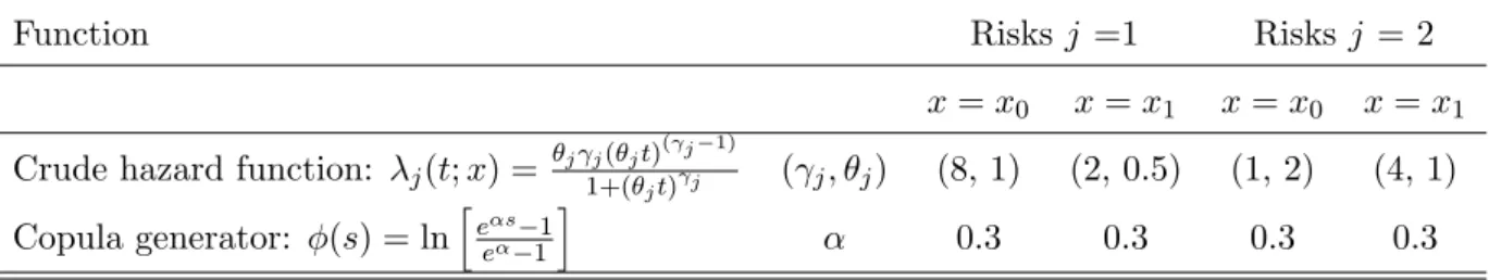
The cause-specific crude hazard functions follow log-logistic distributions with different parameters for eachj and x. The model parameters are given in Table 1. Since we know the trueS, Sj and
Qj for all j, we can easily asses the performance of our identification strategy. We first apply
our identification method to the true values of S, Qj and Sj for all j. Then we asses finite
sample performance when we use nonparametric estimators forS and Qj for all j. Although, the
identification and estimation procedures outlined in the previous section can be applied for any
Table 1: Parameters of the simulated competing risks model.
Function Risksj =1 Risks j = 2
x=x0 x=x1 x=x0 x=x1
Crude hazard function: λj(t;x) = θjγj(θjt)
(γj−1) 1+(θjt)γj (γj, θj) (8, 1) (2, 0.5) (1, 2) (4, 1) Copula generator: ϕ(s) = ln [ eαs−1 eα−1 ] α 0.3 0.3 0.3 0.3
Identifiability Since we know Qj and Sj for all j, it is straightforward to compute (tc,t,`´t),
∆c
xQj(t), ∆mxQj(t), ∆cxFj(t), ∆mxFj(t) and ∆xFj(t) for any t on our grid.
Panels (a) and (b) of Figure 2 show the treatment effect (∆xFj(t)), the Peterson bounds (P Bj)
and the corresponding nonparametric identification setsIPj. It also shows IIj(x) andIDj(x) using
the copula effect and the marginal distribution effect. The sets IPj are plotted as horizontal lines
at -1.2, and IIj(x) and IDj(x) by horizontal lines at -1.3 and -1.4 respectively. The Figure also
contains the identified sign (ISj(x)) as horizontal lines at (1,0,-1) based on the union set of IIj(x),
IDj(x) andIPj. Panels (c) and (d) contain the same sets for the reversed treatment effect ∆−x to
illustrate that the method of Section 2.1 indeed increases the union of all identification sets. It can be seen that the sign of the treatment effect for risk 1 cannot be identified from the Peterson bounds for any t, while for risk 2 a negative treatment effect is identified from duration time zero to one. It is also evident that the resulting identification sets of our procedure are larger than the sets for the Peterson bounds. When we apply the procedure of Section 2.1 to increase the identification set it becomes apparent that it results in rather different sets ISj, which indicates
the usefulness of this procedure. As the sets IP1 and IP2 are only small subsets of Q1 and Q2 respectively, we also gain more insights about the magnitude of the effect as this is bounded by 0 from above (below) for risk 1 (2) fort >1.5.
Estimation Next we simulate data with sample size 500 and estimate Qj and S as outlined in
Section 3 For inference we perform the bootstrap test outlined in Section 3.2 with 500 bootstrap samples and ϵ = 0.01. The estimation results are given in panels (e) and (f) of Figure 2. The
estimated sign (ESj) is plotted as a black horizontal line at (-1,0,1) if the estimate is significant
at the 5% level and it is plotted in grey otherwise. The sets ˆIPj and ˆQj are plotted as horizontal
lines at -1.2 and -1.5 respectively. When we compare the estimation results with the true values in panels (a)-(d), it is evident that there is no bias for the sign estimation and the identification
Figure 2: Identified sign (IS) and estimated sign (ES) of the treatment effect in a known two risks model. risk 1 risk 2 (a) (b) 0 1 2 3 4 5 −1.4 −1.3 −1.2 −1 0 1 t pp ∆xF1 ∆c xQ1 ∆m xQ1 P B1 IS1(x) IP1 II1(x) ID1(x) 0 1 2 3 4 5 −1.5 −1 −0.5 0 0.5 1 time pp t pp ∆xF2 ∆c xQ2 ∆m xQ2 P B2 I S2(x) IP2 II2(x) ID2(x) (c) (d) 0 1 2 3 4 5 −1.4 −1.3 −1.2 −1 0 1 t pp ∆xF1 ∆c −xQ1 ∆m −xQ1 P B1 IS1(−x) IP1 II1(−x) ID1(−x) 0 1 2 3 4 5 −1.5 −1 −0.5 0 0.5 1 t pp ∆xF2 ∆c −xQ2 ∆m −xQ2 P B2 IS2(−x) IP2 II2(−x) ID2(−x) (e) (f) −1.4 −1.2 −1 0 1 pp ∆xF1 ES1(insig) ES1(sig.) ˆ IP1 ˆ Q1 −1.5 −1 −0.5 0 0.5 1 pp ∆xF2 ES2(insig) ES2(sig.) ˆ IP2 ˆ Q2
sets are very similar to the true values.
5
Application
In this section we present an illustrative application to unemployment duration data from Ger-many. For the estimations we use a sample of the scientific use file version of the IAB employment sample (IABS) 2001 of the Institute for Employment Research (IAB). These administrative data are a 2% random sample of the German workforce subject to social security contributions in the period 1975-2001. The IABS contains daily information about periods of dependent employment and claim periods for unemployment compensation along with basic information about the in-dividual (such as gender, wage, age and employment history) and the employing firm (such as business sector and location). For more information on the IABS see Hamann et al. (2004). From these data we extract all unemployment periods starting in 1998 or 1999 and having a foregoing employment period. We define unemployment as receipt of unemployment compensation from the German Federal Employment Agency. This leaves us with a sample of 107,522 observations. We consider a model with two risks: employment and other exits. We analyse the effect of various binary covariate changes such as gender, calendar time and employment history of individuals on the job finding probability. Results for the second risk are not presented as it does not have a direct interpretation.
Figures 3 and 4 present estimated nonparametric cumulative incidence curves, the resulting Peterson bounds and the estimated sign (ES) of the covariate effects on the marginal distribution of job finding. ES is plotted as horizontal lines at -1, 0 and 1 in dark grey if the estimate is significant and in light grey if it is insignificant. It is apparent from the left panels of the figures that estimated CICs change considerably in female, recall, previous unemployment, low wage and winter while the effect of calender year 1999 (instead of 1998) is very small. The estimated Peterson bounds in the right panels are often wide and only partly informative. In the case of female, recall, low wage and winter the set ˆIP1(horizontal line at -1.2) partly covers the interval up
to 150-250 days while it is (almost) empty for other variables. In the case of winter the Peterson bounds suggest a change in the sign of the covariate effect at about 50 days. When applying our identification and estimation approaches of Section 3 the identification set ˆQ1 (horizontal line at -1.5) is much larger than ˆIP1 for all variables. In particular it covers almost the entire set of
durations in the case of female, recall, pervious unemployment and winter. This suggests that the identification set is enlarged substantially by imposing Assumptions 1-3 while still allowing for many different dependence structures. Due to the large sample size the estimated sign is mainly significant. For the calendar time variables winter and year 1999 we find evidence for a change in the sign of the covariate effect as unemployment duration progresses. Even though the estimated CICs for the years 1998 and 1999 are extremely similar, the set Q1 contains almost one third of all
t. For all variables the set IPj is much smaller than the set Qj. For this reason the identification
of the sign of the effect can be also used to derive considerably tighter bounds for the magnitude of the effects for many durations.
Figure 3: Cumulative incidence for job finding (left) and estimated sign of covariate effects on the marginal distribution (right).
Female 0 200 400 600 800 1000 0 0.1 0.2 0.3 0.4 0.5 0.6 0.7 0.8
unemployment duration (in days)
pp ˆ Q1(t,0) ˆ Q1(t,1) 0 200 400 600 800 1000 −1.5 −1 −0.5 0 0.5 1
unemployment duration (in days)
pp ∆c xQˆ1 ∆m xQˆ1 ˆ P B1 ES1(insig.) ES1(sig.) ˆ IP1 ˆ Q1 Recall 0 200 400 600 800 1000 0 0.1 0.2 0.3 0.4 0.5 0.6 0.7 0.8
unemployment duration (in days)
pp ˆ Q1(t,0) ˆ Q1(t,1) 0 200 400 600 800 1000 −1.5 −1 −0.5 0 0.5 1
unemployment duration (in days)
pp ∆c xQˆ1 ˆ ∆m xQ1 ˆ P B1 ES1(insig.) ES1(sig.) ˆ IP1 ˆ Q1 Previous unemployment 0 200 400 600 800 1000 0 0.1 0.2 0.3 0.4 0.5 0.6 0.7 0.8 pp ˆ Q1(t,0) ˆ Q1(t,1) 0 200 400 600 800 1000 −1.5 −1 −0.5 0 0.5 1 pp ∆c xQˆ1 ∆m xQˆ1 ˆ P B1 ES1(insig.) ES1(sig.) ˆ IP1 ˆ Q1
Figure 4: Cumulative incidence for job finding (left) and estimated sign of covariate effects on the marginal distribution (right).
Low wage 0 200 400 600 800 1000 0 0.1 0.2 0.3 0.4 0.5 0.6 0.7 0.8
unemployment duration (in days)
pp ˆ Q1(t,0) ˆ Q1(t,1) 0 200 400 600 800 1000 −1.5 −1 −0.5 0 0.5 1
unemployment duration (in days)
pp ∆c xQˆ1 ∆m xQˆ1 ˆ P B1 ES1(insig.) ES1(sig.) ˆ IP1 ˆ Q1 Winter 0 200 400 600 800 1000 0 0.1 0.2 0.3 0.4 0.5 0.6 0.7 0.8
unemployment duration (in days)
pp ˆ Q1(t,0) ˆ Q1(t,1) 0 200 400 600 800 1000 −1.5 −1 −0.5 0 0.5 1
unemployment duration (in days)
pp ∆c xQˆ1 ∆m xQˆ1 ˆ P B1 ES1(insig.) ES1(sig.) ˆ IP1 ˆ Q1 Year 1999 0 200 400 600 800 1000 0 0.1 0.2 0.3 0.4 0.5 0.6 0.7 0.8 pp ˆ Q1(t,0) ˆ Q1(t,1) 0 200 400 600 800 1000 −1.5 −1 −0.5 0 0.5 1 pp ∆c xQˆ1 ∆m xQˆ1 ˆ P B1 ES1(insig.) ES1(sig.) ˆ IP1 ˆ Q1
Appendix: Proofs
Proof of Lemma 1: 1.(a) The copula effect and the marginal distribution effect in Definitions
1 and 2 are unique for all t if tc is unique. The latter is guaranteed by the invertibility of S(t).
1.(b) Result (4) follows from Definitions 1 and 2:
∆xFj(t) = ∆cxFj(t) + ∆mxFj(t)
=Fj(tc;x1)−Fj(t;x0) +Fj(t;x1)−Fj(tc;x1) =Fj(t;x1)−Fj(t;x0).
In order to prove 1.(c) we first state and prove two additional Lemmas:
Lemma A1 Under Assumptions 1 and 2 in model (1), we have sign|∆cxF1(t)|=−sign|∆cxF2(t)|
for all t.
We prove Lemma A1 by stating the condition for tc and t to satisfy Definitions 1 and 2:
S(t;x0) = C{S1(t;x0), S2(t;x0)}=C{S1(tc;x1), S2(tc;x1)} =S(tc;x1). (17) A survival copula function is increasing in both of its arguments (see Theorems 2.2.7 and 2.4.4 in Nelsen, 2006). Then the copula effect of risk 1 being positive, i.e. S1(tc;x1) < S1(t;x0), implies
the copula effect of risk 2 being negative as S2(tc;x1)< S2(t;x0) is required for condition (17) to hold. Similar reasoning applies if the copula effect of risk 1 is negative and and the copula effect of risk 2 is positive. This proves that the copula effects for risk 1 and risk 2 have different signs for all t unless both are zero.
Lemma A2 Under Assumptions 1 and 2 in model (1), we have sign|∆m
xF1(t)|=sign|∆mxF2(t)|
for all t.
Lemma A2 bases on Lemma A1 in Zheng and Klein (1995) which suggests that s2 = ζ21(s1;x)
is unique. This guarantees uniqueness of s2 = ζ21(s1;x) for any given value s1 and vice versa.
ζ21(s1;x) is therefore a strictly increasing function in s1 for all x. Suppose we have F1(ta;x) <
F1(tb;x) for any ta, tb ∈ IT and thus S1(ta;x) > S1(tb;x). Then by s2 = ζ21(s1;x) being strictly increasing, we also have S2(ta;x) > S2(tb;x), and thus F2(ta;x) < F2(tb;x). The same reasoning
applies to the cases ofF1(ta;x)> F1(tb;x) or F1(ta;x) = F1(tb;x), which completes the proof.
These results are now used to prove 1.3). According to (4), the sign of ∆xF1(t) is determined
by the sign of the copula and the marginal distribution effect if {sign|∆c
belongs to one of the following combinations: {1,1}, {1,0}, {0,1}, {0,0}, {-1,-1},{-1,0}or {0,-1}. Otherwise ∆c
xF1(t) and ∆mxF1(t) have opposite signs, and in these cases the sign of ∆xF1(t) is undetermined (or ambiguous). In case ∆cxFj(t) = 0 for j = 1,2 or ∆mxFj(t) = 0 for j = 1,2, the
sign of ∆xF1(t) and ∆xF2(t) are unambiguously determined. If both the copula and the marginal
distribution effects are nonzero, we first consider the case that both ∆cxF1(t) and ∆mxF1(t) have the same sign. In this case, the sign of ∆xF1(t) is determined but not the sign of ∆xF2(t). It is because
−sign|∆cxF2(t)| = sign|∆cxF1(t)| = sign|∆mxF1(t)| = sign|∆mxF2(t)| according to Lemmas A1 and A2. Analogous reasoning applies if sign of ∆c
xF1(t) and ∆mxF1(t) are different. As in this case, the sign of ∆xF2(t) is determined but not the sign of ∆xF1(t). It follows that sign|∆xFj(t)| can
be always determined for at least one j fromsign|∆m
xFj(t)| and sign|∆xmFj(t)| for all t∈IT.
Lemma A3 Under Assumptions 1 and 2 in model (1), if there is some subset of duration time
M ⊆ IT such that the link function is monotone in all t ∈ M, we have Z(t) = ζ{S1(t);x1 −
S1(t);x0} > 0 or Z(t) < 0 for all t ∈ M. Then Z(t) > 0 implies ∆cxF1(t) > 0 and Z(t) < 0
implies ∆c
xF1(t)<0 for all t ∈M.
The proof of Lemma A3 uses Lemma A1 and Lemma A2. As the copula effect for risks 1 and 2 has an opposite sign for all t, we show that ∆c
xF1(t;x1) cannot be negative if Z(t) > 0. This is because ∆cxF1(t;x1) < 0 implies ∆cxF2(t;x1) > 0, which means that S1(tc;x1) > S1(t;x0) and
S2(tc;x1) < S2(t;x0) at all t. For some t > tc we have S2(t;x1) < S2(tc;x1). Moreover we know
from Lemma A2 that there exists a t such that S1(t;x1) < S1(tc;x1) and fulfills the condition
S1(t;x1) =S1(t;x0). Putting this together,
ζ21(S1(t;x1);x1) =S2(t;x1)< S2(t;x0) =ζ21(S1(t;x0);x0) = ζ21(S1(t;x1);x0).
This contradicts the initial conditionZ(t)>0 which requiresζ21(s1;x1)> ζ21(s1;x0) for all s1.
Proof of Lemma 3: The proof comprises several steps. First, we define a sequence {t˙k} and
state several useful properties of it in Lemma A4. Second, we show that sign of the copula effect can be identified, if {t˙k} was known (Lemma A5). Third, the unobserved ˙t can be bounded
by intervals with observed endpoints [`tk,t´k] (Lemma A6). Fourth, we use these results to prove
Lemma 3.
Definition A1 We denote{t˙k} ∈IT fork = 0,1,2, . . . as a finite sequence of durationst at which
Z( ˙tk) = ζ21{S1( ˙tk);x1} −ζ21{S1( ˙tk);x0} = 0 and sign|limt→+t˙
kZ(t)| ̸= sign|limt→−t˙kZ(t)| for
all k >0. We define t˙0 = 0 and the corresponding sequence {t˙ck} for the duration time tc defined
in Definition 1 such that S( ˙tc
k;x1) =S( ˙tk;x0) for all k.
Lemma A4 Under Assumptions 1 and 2, {t˙k} ∈IT has the following properties:
1. The link function S2(t) = z21{S1(t);x} at any t ∈ ( ˙tk,t˙k+1) ≡ IT˙k, is a strictly monotone
function in x, i.e. either (i) Z(t) < 0 or (ii) Z(t) > 0 for t ∈ IT˙k and for all k. The link
function is, however, generally non-monotone at any t∈ {t˙m,t˙n}, for any 1< m+ 1< n.
2. The copula effect at {t˙k} is zero for all k and all risks j, i.e.
∆cxFj( ˙tk) = Fj( ˙tkc;x1)−Fj( ˙tk;x0) = 0;
thus Sj( ˙tck;x1) =Sj( ˙tk;x0). (18)
3. The copula effect on the CIC at {t˙k} is nonzero for any k >0 and all risks j,
∆cxQj( ˙tk) = Qj( ˙tk;x1)−Qj( ˙tk;x0)̸= 0. (19)
4. For any t∈( ˙tk,t˙k+1) and k > 0,
A1(t) = ∫ ζ21(s1; x1) 0 ∫ S1( ˙tck; x1) S1(tc; x1) C′′ ds1 ds2− ∫ ζ21(s1; x0) 0 ∫ S1( ˙tk; x0) S1(t;x0) C′′ ds1 ds2. ∝ ∆cxF1(t;x). (20)
Lemma A4.1 holds for any link functions2 =ζ21(s1) that is strictly increasing ins1. According to Definition A1Z(t) changes its sign at all{t˙k}. Lemma A4.2 can be proved by Definitions 1 and
A1. [S1( ˙tck;x1), S2( ˙tkc;x1)] is the solution to (i)C{S1( ˙tck;x1), S2( ˙tck;x1)}=C{S1( ˙tk;x1), S2( ˙tk;x1)}, (ii) S2( ˙tck;x1) = ζ21{S1( ˙tck;x1);x1}, and (iii) ζ21{S1( ˙tck;x1);x1} = ζ21{S1( ˙tk;x0);x0}. (ii) and (iii) implyS2( ˙tck;x1) = S2( ˙tk;x0). As the copula function is strictly increasing in both of its arguments,
equation (i) holds only if S1( ˙tck;x1) = S1( ˙tk;x1). This leads to equation (18) and completes the proof of Lemma A4.2. Lemma A4.3 can be proved by rewriting ∆c
xQ1( ˙tk) as ∆cxQ1( ˙tk) = Q1( ˙tck;x1)−Q1( ˙tk;x0) = ∫ ζ21(s1;x1) 0 ∫ 1 S1( ˙tck;x1) C′′ ds1 ds2− ∫ ζ21(s1;x0) 0 ∫ 1 S1( ˙tk;x0) C′′ ds1 ds2 = ∫ ζ21(s1;x1) ζ21(s1;x0) ∫ 1 S1( ˙tk;x0) C′′ ds1 ds2. (21)
The last equality follows from (18). As ζ21(s1;x0) equals to ζ21(s1;x1) only at ˙tl and ˙tcl, for all
0≤l ≤k, respectively,Z(t) is nonzero at allt∈[0,t˙k]. Th is completes the proof of Lemma A4.3.
Lemma A4.4 can be shown by using equation (18) and the monotonicity property in Lemma A4.1, which implies that (i) Z(t)< 0 or (ii) Z(t)> 0 for all t ∈ ( ˙tk,t˙k+1). Case (i) implies a negative ∆c
xF1(t) as a result from Lemma A3 and A1(t) in (20) becomes
A1(t) = ∫ ζ21(s1;x1) 0 ∫ S1( ˙tk; x0) S1(tc; x1) C′′ ds1 ds2− ∫ ζ21(s1;x0) 0 ∫ S1( ˙tk;x0) S1(t;x0) C′′ ds1 ds2 < ∫ ζ21(s1;x0) 0 ∫ S1( ˙tk; x0) S1(tc; x1) C′′ ds1 ds2− ∫ ζ21(s1;x0) 0 ∫ S1( ˙tk;x0) S1(t;x0) C′′ ds1 ds2 < ∫ ζ21(s1;x0) 0 ∫ S1( ˙tk; x0) S1(t; x0) C′′ ds1 ds2− ∫ ζ21(s1;x0) 0 ∫ S1( ˙tk;x0) S1(t;x0) C′′ ds1 ds2 = 0.
This completes the proof of Lemma A4.4.
Lemma A5 Under Assumptions 1 and 2, we have for any t with t˙k =sup{t˙l|t˙l≤t},
∆cxQj(t) = ∆cxQj( ˙tk) +Aj(t); and (22)
sign|∆cxFj(t)| = sign∆cxQj(t)−∆cxQj( ˙tk).
for j = 1,2, where πc
j(t)>0 and t˙l as in Definition A1.
distin-guishing between the following two intervals fort ∈(0, t] = (0,t˙k] ∪ ( ˙tk, t]. Then ∆cxQ1(t) = Q1(tc;x1)−Q1(t;x0) = ∫ ζ21(s1;x1) 0 ∫ 1 S1(tc;x1) C′′ ds1 ds2− ∫ ζ21(s1; x0) 0 ∫ 1 S1(t; x0) C′′ ds1 ds2; = ∫ ζ21(s1;x1) 0 ∫ S1( ˙tck; x1) S1(tc;x1) C′′ ds1 ds2+ ∫ ζ21(s1;x1) 0 ∫ 1 S1( ˙tck; x1) C′′ ds1 ds2 − ∫ ζ21(s1;x0) 0 ∫ S1( ˙tk;x0) S1(t;x0) C′′ ds1 ds2− ∫ ζ21(s1; x0) 0 ∫ 1 S1( ˙tk;x0) C′′ ds1 ds2; = A1(t) + ∆cxQ1( ˙tk).
The last line follows from (19) and the definition of A1(t) in Lemma A4.4. According to Lemma
A4.4, the sign of A1(t) is equal to the sign of ∆cxF1(t). And thus ∆cxF1(t) has the same sign as ∆c
xQ1(t)−∆cxQ1( ˙tk) for any t such that ˙tk =sup{t˙l|t˙l ≤t}. This completes the proof of Lemma
A5.
Lemma A6 t˙l ∈[`tk,t´k] for l ≥k and for all k.
In order to prove Lemma A6, we show that ∆c
xQj(t) has at least one local maximum (or minimum)
for all t ∈ IT. This is when the link function ζ21(S1(t);x) is not monotone in x for all t ∈ IT according to Lemma A4.1.
First, we consider the interval t ∈ (0,t˙1) ≡ IT˙0. From (22), we have ∆cxQ1(t) = A1(t). We know from Lemma A4.4 that ∆c
xQ1(t) has the same sign as ∆cxF1(t). Without lost of generality, we consider the case Z(t) >0 for all t ∈IT˙0. According to Lemma A3 we have ∆cxF1(t) <0, and thus ∆c
xQ1(t)<0 for all t in the first interval ˙IT0. The same is true for t= ˙t1 and ∆cxQ1( ˙t1)<0. Next, we consider the interval t ∈( ˙t1,t˙2)≡IT˙1. Using Definition A1, Z(t) changes its sign in ˙IT1, and thusZ(t)<0. It follows that ∆c
xF1(t) changes its sign and becomes positive. From (22) and Lemma A4.4, att∈IT1,
∆cxQ1(t) = ∆cxQ1( ˙t1) +A1(t)> ∆cxQ1( ˙t1).
While we don’t know whether ∆c
xQ1(t) <0 reaches its local minimum and starts to move up at some `t1 (see Definition 5) prior to ˙t1, `t1 should be no later than ˙t1. We therefore have `t1 ∈(0,t˙1] and thus `t1 ≤ t˙1. At ˙t2, ∆cxQ1( ˙t2) = ∆cxQ1( ˙t1) +A1( ˙t2). It is unclear whether |A1( ˙t2)| is large enough to change the sign of ∆c
case where|A1( ˙t2)| ≥ |∆cxQ1( ˙t1)|and ∆cxQ1( ˙t2) is positive. Since ∆cxQ1( ˙t1)<0 and ∆cxQ1( ˙t2)≥0, there exists a ´t1 such that ∆cxQ1(´t1) = 0 with ´t1 ∈( ˙t1,t˙2]. It implies that ˙t1 <´t1.
Combining the above results ˙t1 can be bounded by an interval with observable endpoints [`t1,´t1). In the case where |A1( ˙t2)| < |∆cxQ1( ˙t1)|, ´t1 is only known to be in the interval ˙IT1,IT˙3 or , ˙IT5, . . .. This is because A1(t) is positive only in these intervals and thus only when ´t1 is inside these intervals that could turn ∆c
xQ1(t) to be positive. If, for instance, the actual ´t1 is inside the interval ˙IT3, the three unknowns ˙t1,t˙2 and ˙t3 and not just ˙t1 are bounded by [`t1,t´1). This, however, does not affect the identifiability of `tk and ´tk for all k and the identification results of Lemma 3,
except that the identification region will be reduced. The above reasoning can be carried over to all ˙tk which completes the proof of Lemma A6.
We now prove Lemma 3 for different intervals oftby using Lemma A6. For simplicity we focus on the case ˙tk ∈[`tk,´tk] for allk. For t∈[0,t˙1], sign|∆cxFj(t)|=sign|∆cxQj(t)| as already shown.
The lower bound of ˙t1 is `t1 and ´t0 = 0. Thus, Lemma 3 holds for t ∈ [´t0,`t1]. For t ∈ [ ˙t1,t˙2], we observe only the upper bound of ˙t1 and the lower bound of ˙t2 which is the interval [´t1,t`2].
According to Definition 5, we have the following bounds for ∆cxQ1(t) fort ∈[´t1,`t2]: ∆cxQ1(´t1)<∆cxQ1(t)<∆cxQ1(`t2) for ∆xcQ1(`t2)>0;
∆cxQ1(´t1)>∆cxQ1(t)>∆cxQ1(`t2) for ∆xcQ1(`t2)<0.
And with ∆cxQ1(´t1) = 0 and Lemma A5, we have
0<∆cxQ1(t)<∆cxQ1( ˙t1) +A1(`t2) for ∆xcQ1(`t2)>0;
0>∆cxQ1(t)>∆cxQ1( ˙t1) +A1(`t2) for ∆cxQ1(`t2)<0.
Note that ∆cxQ1(t) is zero at ´t1 with ´t1 ∈ ( ˙t1,t`2) and thus ∆cxQ1( ˙t1) and ∆cxQ1(`t2), which are nonzero, must have different directions. It follows that
0<∆cxQ1(t)< A1(`t2) for ∆cxQ1(`t2)>0
0>∆cxQ1(t)> A1(`t2) for ∆cxQ1(`t2)<0.
Using Lemma A4.4, completes the proof of Lemma 3 fort∈[´t1,`t2]. The proof is analogous for all
other values of k.
Proof of Corollary 1: We first state a Lemma that is required for the proof. As Fj(t;x) is