Clique Using
o(m)
Messages
∗
Sriram V. Pemmaraju
1and Vivek B. Sardeshmukh
21 Department of Computer Science, University of Iowa, Iowa City, USA
2 Department of Computer Science, University of Iowa, Iowa City, USA
Abstract
In a sequence of recent results (PODC 2015 and PODC 2016), the running time of the fastest algorithm for theminimum spanning tree (MST)problem in theCongested Cliquemodel was first improved toO(log log logn) fromO(log logn) (Hegeman et al., PODC 2015) and then toO(log∗n) (Ghaffari and Parter, PODC 2016). All of these algorithms use Θ(n2) messages independent of
the number of edges in the input graph.
This paper positively answers a question raised in Hegeman et al., and presents the first “super-fast” MST algorithm witho(m) message complexity for input graphs withmedges. Specifically, we present an algorithm running inO(log∗n) rounds, with message complexity O(e
√
m·n) and then build on this algorithm to derive a family of algorithms, containing for anyε, 0< ε≤1, an algorithm running inO(log∗n/ε) rounds, usingO(ne 1+ε/ε) messages. Settingε= log logn/logn
leads to the first sub-logarithmic round Congested Clique MST algorithm that uses onlyO(n)e
messages.
Our primary tools in achieving these results are
(i) a component-wise bound on the number of candidates for MST edges, extending the sampling lemma of Karger, Klein, and Tarjan (Karger, Klein, and Tarjan, JACM 1995) and
(ii) Θ(logn)-wise-independent linear graph sketches (Cormode and Firmani, Dist. Par. Databases, 2014) for generating MST candidate edges.
1998 ACM Subject Classification F.2.0 [Analysis of Algorithms and Problem Complexity] Gen-eral, C.2.4 [Computer-Communication Networks] Distributed Systems
Keywords and phrases Congested Clique, Minimum Spanning Tree, Linear Graph Sketches, Message Complexity, Sampling
Digital Object Identifier 10.4230/LIPIcs.FSTTCS.2016.47
1
Introduction
TheCongested Clique is a synchronous, message-passing model of distributed computing in which the underlying network is a clique and in each round, a message of size O(logn) bits can be sent in each direction across each communication link. The Congested Clique is a simple, clean model for studying the obstacles imposed by congestion – all relevant information is nearby in the network (at most 1 hop away), but may not be able to travel to an intended node due to the O(logn)-bit bandwidth restriction on the communication links. There has been a lot of recent work in studying various fundamental problems in the Congested Clique model, including facility location [9, 3],minimum spanning tree (MST)
∗ This work is supported in part by National Science Foundation grant CCF 1318166.
© Sriram V. Pemmaraju and Vivek B. Sardeshmukh; licensed under Creative Commons License CC-BY
[23, 13, 11, 10], shortest paths and distances [4, 14, 26], triangle finding [7, 6], subgraph detection [7], ruling sets [3, 13], sorting [28, 22], and routing [22]. The modeling assumption in solving these problems is that the input graphG= (V, E) is “embedded” in the Congested Clique – each node ofGis uniquely mapped to a machine and the edges ofGare naturally mapped to the links between the corresponding machines (see Section 1.1).
The earliest non-trivial example of a Congested Clique algorithm is thedeterministic
MST algorithm that runs in O(log logn) rounds due to Lotker et al. [23]. Using linear sketching[1, 2, 15, 24, 5] and the samplingtechnique due to Karger, Klein, and Tarjan [16], Hegeman et al. [11] were able to design a substantially faster,randomized Congested Clique MST algorithm, running inO(log log logn) rounds. Soon afterwards, Ghaffari and Parter [10] designed anO(log∗n)-round algorithm, using the techniques in Hegeman et al., but supplemented with the use ofsparsity-sensitive sketching, which is useful for sparse graphs andrandom edge sampling, which is useful for dense graphs.
Our Contributions. All of the MST algorithms mentioned above, essentially use the entire bandwidth of the Congested Clique model, i.e., they use Θ(n2) messages. From these examples, one might (incorrectly!) conclude that “super-fast” Congested Clique algorithms are only possible when the entire bandwidth of the model is used. In this paper, we focus on the design of MST algorithms in the Congested Clique model that have lowmessage complexity, while still remaining “super-fast.” Message complexity refers to the number of messages sent and received by all machines over the course of an algorithm; in many applications, this is the dominant cost as it plays a major role in determining the running time and auxiliary resources (e.g., energy) consumed by the algorithm. In our main result, we present an O(log∗n)-round algorithm that usesO(e
√
m·n) 1 messages for an n-node, m-edge input graph. Two points are worth noting about this message complexity upper bound: (i) it is bounded above by O(ne 1.5) for all values of m and is thus substantially
sub-quadratic, independent ofmand (ii) it is bounded above byo(m) for all values ofmthat are super-linear inn, i.e., whenm=ω(npoly(logn)). We then extend this result to design a family of algorithms parameterized byε, 0< ε≤1, and running inO(log∗n/ε) rounds and usingO(ne 1+ε/ε) messages. If we setε= log logn/logn, we get an algorithm running
inO(log∗n·logn/log logn) rounds and usingO(n) messages. Thus we demonstrate thee
existence of a sub-logarithmic round MST algorithm using onlyO(n·poly(logn)) messages, positively answering a question posed in Hegeman et al. [11]. We note that Hegeman et al. present an algorithm using O(n) messages that runs ine O(log5n) rounds. All of the
round and message complexity bounds mentioned above hold with high probability (w.h.p.), i.e., with probability at least 1−1
n. Our results indicate that the power of the Congested Clique model lies not so much in its Θ(n2) bandwidth as in the flexibility it provides – any communication link that is needed is present in the network, though most communication links may eventually not be needed.
Applications. Optimizing message complexity as well as time complexity for Congested Clique algorithms has direct applications to the performance of distributed algorithms in other models such as the Big Data (k-machine) model [18], which was recently introduced to study distributed computation on large-scale graphs. Via a Conversion Theorem in [18] one can obtain fast algorithms in the Big Data model from Congested Clique algorithms that
1 The notation
e
have low time complexityand message complexity. Another related motivation comes from the connection between the Congested Clique model and the MapReduce model. In [12] it is shown that if a Congested Clique algorithm runs inT rounds and, in addition, has moderate message complexity then it can be simulated in the MapReduce model inO(T) rounds.
1.1
Technical Preliminaries
Congested Clique model. TheCongested Cliqueis a set ofncomputing entities (nodes) connected through a complete network that provides point-to-point communication. Each node in the network has a distinct identifier of O(logn) bits. At the beginning of the computation, each node knows the identities of allnnodes in the network and the part of the input assigned to it. The computation proceeds in synchronous rounds. In each round each node can perform some local computation and send a (possibly different) message ofO(logn) bits to each of itsn−1 neighbors. It is assumed that both the computing entities and the communication links are fault-free. The Congested Clique model is therefore specifically geared towards understanding the role of the limited bandwidth as a fundamental obstacle in distributed computing, in contrast to other classical models for distributed computing that instead focus, e.g., on the effects of latency (theLocalmodel) or on the effects of both latency and limited bandwidth (theCongestmodel).
The input graph is assumed to be a spanning subgraph of the underlying communication network. Before the algorithm starts, each node knows the edges of the input graph incident on it and their (respective) weights. We assume that every edge weight can be represented withO(logn) bits. For ease of exposition, we assume that edge weights are distinct; otherwise, without loss of generality (WLOG) we can “pad” each edge weight with the IDs of the two end points of the edge so as to distinguish the edges by weight while respecting their weight-based ordering. We require that when the algorithm ends, each node knows which of its incident edges belong to the output MST.
Linear Sketches. A key tool used by our algorithm is linear sketches [1, 2, 24]. Let av denote a vector whose non-zero entries represent edges incident onv. Alinear sketchofavis a low-dimensional random vectorsv, typically of sizeO(poly(logn)), with two properties:
(i) sampling from the sketchsv returns a non-zero entry of av with uniform probability (over all non-zero entries inav) and
(ii) when nodes in a connected component are merged, the sketch of the new “super node” is obtained by coordination-wise addition of the sketches of the nodes in the component. The first property is referred to as`0-sampling in the streaming literature [5, 24, 15] and the second property islinearity. The graph sketches used in [1, 2, 24] rely on the`0-sampling algorithm by Jowhari et al. [15]. Sketches constructed using the Jowhari et al. [15] approach use Θ(log2n) bits per sketch, but require polynomially many mutually independent random bits to be shared among all nodes in the network. Sharing this volume of information is not feasible; it takes too many rounds and too many messages. So instead, we appeal to the `0-sampling algorithm of Cormode and Firmani [5] which requires a family of Θ(logn)-wise independent hash functions, as opposed to hash functions with full-independence. Hegeman et al. [11] provide details of how the Cormode-Firmani approach can be used in the Congested Clique model to construct graph sketches. We summarize their result in the following theorem.
ITheorem 1.1(Hegeman et al. [11]). Given an input graphG= (V, E), n=|V|, there is a Congested Clique algorithm running inO(1) rounds and usingO(n·poly(logn))messages,
at the end of which every node v ∈V has computed a linear sketch sv of av. The size of
the computed sketch of a node is O(log4n) bits. The`0-sampling algorithm on sketch sv
succeeds with probability at least 1−n−2 and, conditioned on success, returns an edge ina v
with probability in the range[1/Lv−n−2,1/Lv+n−2], whereLv is the number of non-zero
entries in av.
Concentration Bounds for sums of k-wise-independent random variables. The use of k-wise-independent random variables, fork= Θ(logn), plays a key role in keeping the time and message complexity of our algorithms low. The use of Θ(logn)-wise independent hash functions in the construction of linear sketches has been mentioned above. In the next subsection, we discuss the use of Θ(logn)-wise-independent edge sampling as a substitute for the fully-independent edge sampling of Karger, Klein, and Tarjan. For our analysis we use the following concentration bound on the sum ofk-wise independent random variables, due to Schmidt et al. [33] and slightly simplified by Pettie and Ramachandran [31].
ITheorem 1.2(Schmidt et al. [33]). LetX1, X2, . . . , Xn be a sequence of randomk-wise
independent 0-1 random variables withX =Pn
i=1Xi. Ifk≥2 is even andC≥E[X]then:
P r(|X−E[X]| ≥T)≤h√2 coshpk3/36Ci· kC eT2 k/2 .
We use the above theorem fork= Θ(logn) andC=T =E[X]. Furthermore, in all instances in which we use this bound,E[X]> k3 and therefore the contribution of the cosh(·) term is O(1), whereas the contribution of the second term on the right hand side is smaller than 1/nc for any constantc.
MST with Linear Message Complexity. The “super-fast” MST algorithms mentioned so far [23, 11, 10] use Θ(n2) messages, independent of the number of edges in the input graph. One reason for this is that these algorithms rely on deterministic constant-round Congested Clique algorithms for routing and sorting due to Lenzen [22]. Lenzen’s algorithms do not attempt to explicitly conserve messages and need Ω(n1.5) messages independent of the number of messages being routed or the number of keys being sorted. However, the above-mentioned MST algorithms do not need the full power of Lenzen’s algorithms. We design sorting and routing protocols that work in slightly restricted settings, but use only a linear number of messages (i.e., linear in the total number messages to be routed or keys to be sorted). Details of these protocols appear in the full version of the paper [30]. We use these protocols (instead of Lenzen’s protocols) as subroutines in the Ghaffari-Parter MST algorithm [10] to derive a version that uses only linear (up to a polylogarithmic factor) number of messages.
ITheorem 1.3(LinearMessages-MST). There exists a Congested Clique MST algorithm running inO(log∗n)rounds using O(m)e messages w.h.p. on an input graph withnnodes
andm edges.
1.2
Algorithmic Overview
The high-level structure of our algorithm is simple. Suppose that the input is ann-node, m-edge graphG= (V, E). We start by sparsifyingGby sampling each edge with probability pand compute amaximal minimum weight spanning forestFof the resulting sparse subgraph H. Thus H containsO(m·p) edges w.h.p. Now consider an edge{u, v} inGand add it toF; if F +{u, v} contains a cycle and {u, v} is the heaviest edge in this cycle, then by
Tarjan’s “red rule” [34] the MST ofGdoes not contain edge {u, v}. Ignoring all such edges leaves a set of edges that are candidates for being in the MST. We appeal to the well-known sampling lemma due to Karger, Klein, and Tarjan [16] (KKT sampling) that provides an estimate of the size of this set of candidates.
IDefinition 1.4 (F-light edge [16]). LetF be a forest in a graphGand letF(u, v) denote the path (if any) connectinguandvin F. LetwF(u, v) denote the maximum weight of an edge onF(u, v) (if there is no path thenwF(u, v) =∞). We call an edge{u, v} F-heavy if w(u, v)> wF(u, v), andF-light otherwise.
I Lemma 1.5 (KKT Sampling Lemma [16]). Let H be a subgraph obtained from G by including each edge independently2 with probability p and letF be the maximal minimum weight spanning forest of H. The number of F-light edges inGis at mostn/p, w.h.p.
As our next step we compute the set of F-light edges and in our final step, we compute an MST of the subgraph induced by the F-light edges. Thus, at a high level, our algorithm consists of two calls to an MST subroutine on sparse graphs, one withO(m·p) edges and the other with O(n/p) edges. In between, these two calls is the computation of F-light edges. This overall algorithmic structure is clearly visible in Lines 5–7 in the pseudocode in Algorithm 1 MST-v1.
There are several obstacles to realizing this high-level idea in the Congested Clique model in order to obtain an algorithm that is “super-fast” and yet has low message complexity. The reason for sparsifyingGand appealing to the KKT Sampling Lemma is the expectation that we would need to use fewer messages to compute an MST on a sparser input graph. However, as mentioned earlier, all of the existing “super-fast” MST algorithms use Θ(n2) messages and are insensitive to the number of edges in the input graph. In our first contribution, we develop a collection of simple, low-message-complexity distributed routing and sorting subroutines that we can use in the Ghaffari-Parter MST algorithm, allowing us to complete the two calls to the MST subroutine inO(log∗n) rounds using max{O(m·p), O(n/p)}messages. Setting the sampling probabilitypin our algorithm topn
m balances the two terms in the max(·,·) and yields a message complexity ofO(√m·n). Due to space restrictions, this contribution is briefly mentioned in Section 1.1 and is described in detail in the full version of our paper [30]. Our second andmain contribution (Section 3) is to show that the computation ofF-light can be completed in O(1) rounds, while still using O(e
√
m·n) messages. To explain the challenge of this computation we present two simple algorithmic scenarios:
Suppose that we want each nodeuto perform a local computation to determine which of its incident edges fromGareF-light. To do this, nodeuneeds to knowwF(u, v) for all neighborsv. Thusuneeds degreeG(u) pieces of information and overall this approach seems to require the movement of Ω(m) pieces of information, i.e., Ω(m) messages. Alternately, we might want each node that knowsF to be responsible for determining which edges inGareF-light. In this case, the obvious approach is to send queries of the type “Is edge{u, v}F-light?” to nodes that knowF. This approach also requires Ω(m) messages.
Various combinations of and more sophisticated versions of these ideas also require Ω(m) messages. So the fundamental question is how do we determine the status (i.e., F-light or
2 For reasons that will become clear later, our goal of keeping the message complexity low, does not allow
us to assume full independence in this sampling. Instead we use Θ(logn)-wise independent sampling and show that a slightly weaker version of the KKT Sampling Lemma holds even with limited independence sampling.
F-heavy) ofm edges while exchanging far fewer thanm messages? Below we outline two techniques we have developed in order to answer this question.
Component-wise bound on number ofF-light edges. As mentioned above, the KKT Sam-pling Lemma upper bounds the total number of F-light edges by O(n/p), which is O(√m·n) for p= pn/m. We show (in Corollary 3.5) that a slightly weaker bound (weaker by a logarithmic factor) holds even if the edge-sampling is done using an Θ(log n)-wise-independent sampler. If we could ensure that the total volume of communication is proportional to the number ofF-light edges, we would achieve our goal ofo(m) message complexity. To achieve this goal we show that the set ofF-light edges has additional structure; they are “evenly distributed” over the components ofF. To understand this imagine thatF is constructed fromH using Bor˘uvka’s algorithm. LetCi={Ci
1, C2i, . . .} be the set of components at the beginning of a phase i of the algorithm. For each componentCji ∈ Ci, the algorithm picks aminimum weight outgoing edge (MWOE)ei j from F. Components are merged using edges ei
j, j= 1,2, . . . and we get a new set of componentsCi+1. LetLi
j be the set of edges inGleaving componentC i
j with weight at
mostw(ei
j). We show in Lemma 3.4 that the set of allF-light edges is just the union of theLi
j’s, over all phasesiand components j within Phasei. Furthermore, we show in Lemma 3.2 that the size ofLi
j for any i, j is is bounded by O(1/p) w.h.p. This “evene
distribution” ofF-light edges suggests that we could make each componentCjiresponsible for identifying the Li
j-edges. Note that we don’t use distributed Bor˘uvka’s algorithm to compute F because that would take Θ(logn) rounds. We computeF inO(log∗n) rounds usingLinearMessages-MST, the modified Ghaffari-Parter MST algorithm (see Theorem 1.3.). F is then gathered at each of a small number of nodes and each node who knowsF completely simulates Bor˘uvka’s algorithmlocally on F, thus identifying the componentsCi
j and their MWOE’seij.)
Component-wise generation of F-light edges using linear sketches. Linear sketches play a key role in helping nodes in each componentCi
j collectively compute all edges inLij. For any nodev and numberx, letNx(v) denote the set of neighbors ofv that are connected tovvia edges of weight less thanx. Each nodev∈Ci
j computes aw(eij)-restricted sketch
sv, i.e., a sketch of its neighborhoodNw(ei
j), and sends it to the component leader of Ci
j who aggregates these sketches to compute a single component sketch. Sampling this sketch yields a single edge inLi
j. SinceLij hasO(1/p) edges, each nodee v∈Cji can send e
O(1/p) separatew(ei
j)-restricted sketches to the component leader ofCji and the Coupon Collector argument ensures that this volume of sketches is enough to generateall edges incident inLi
j w.h.p.
IRemark. The sampling approach of Karger, Klein, and Tarjan is used in a somewhat minor way in earlier Congested Clique MST algorithms [10, 11] and in fact in [19] it is shown that this sampling approach can be replaced by a simple, deterministic sparsification. However, KKT sampling and specifically its Θ(logn)-wise independent version that we use in the current algorithm seems crucial for ensuring low message complexity, while keeping the algorithms fast.
1.3
Related Work
It is important to point out that our algorithms are designed for the so-called KT1 [29] model, where every node initially knows the IDs of all its neighbors, in addition to its own ID. (In the Congested Clique model, this means that each node knows the IDs of allnnodes in
nodes are unaware of IDs of neighbors, then it has been shown in [11] that Ω(m) messages are needed by any Congested Clique MST algorithm (including randomized Monte Carlo algorithms, and regardless of the number of rounds) on an m-edge input graph. In fact, this lower bound is shown for the simpler graph connectivity problem.
There have also been some recent developments on simultaneously optimizing message complexity and round complexity for the MST problem in theCongestmodel. For example, in [27] it is shown that there exists a randomized (Las Vegas) algorithm that runs in
e
O(√n+ diameter(G)) rounds and usesO(m) messages (both w.h.p.). This improves thee
message complexity of the well-known Kutten-Peleg algorithm [21], without sacrificing round complexity (up to polylogarithmic factors). The Kutten-Peleg algorithm runs in O(√nlog∗n+ diameter(G)) rounds, while using O(m+n1.5) messages. Note that the algorithm in [27] simultaneously matches the round complexity lower bound [8, 32] and the message complexity lower bound [20] for the MST problem.
The above-mentioned upper and lower bound results assume the KT0 model. In the KT1 model, the message complexity lower bound of Kutten et al. [20] does not hold and King et al. [17] were able to design an MST algorithm in the KT1 Congestmodel that usesO(n) messages, though this algorithm has significantly higher round complexity thane
e
O(√n+ diameter(G)) rounds.
As mentioned earlier, Hegeman et al. [11] present a Congested Clique MST algorithm usingO(n) messages, but running ine O(log5n) rounds. One can make a few changes to the
King et al. [17]Congest-model algorithm to implement it in the Congested Clique model, requiringO(n) messages, but running ine O(log2n/log logn) rounds.
2
MST Algorithms
In this section we describe two “super-fast” MST algorithms, the first runs in O(log∗n) rounds, usingO(e
√
m·n) messages and the second algorithm running inO(log∗n/ε) rounds, usingO(ne 1+ε/ε) messages, for any 0< ε≤1.
2.1
A super-fast algorithm using
O
f(
√
mn
)
messages
Our first algorithm MST-v1, shown in Algorithm 1 has already been outlined in Sec-tion 1.2. The correctness, time complexity, and message complexity of this algorithm depends mainly on two subroutines: LinearMessages-MST(·) andCompute-F-Light(·). Recall that LinearMessages-MST(H) computes an MST on an n-node m-edge input graph H in O(log∗n) rounds using O(m) messages (Theorem 1.3). We also show thate
Compute-F-Light(G, F, p) terminates inO(1) rounds usingO(n/p) messages w.h.p. Thise
is the main result in our paper and is shown in Section 3.
I Lemma 2.1. For some constants c1, c2 > 1, (i) Pr(|E(H)| > c1 ·√mn) < n1 and (ii) Pr(|E`|> c2·
√
mnpoly(logn))< n1.
Proof. For 0 < i ≤ m, let Xi = 1 if edge i is sampled. Hence |E(H)| = PiXi and
E[|E(H)|] =√mn. Note thatXi’s are Θ(logn)-wise independent. Therefore, by Theorem 1.2 we have, Pr(|E(H)|> c1√mn)< 1n for some suitable constant c1 >1. Claim (ii) follows
from Corollary 3.5. J
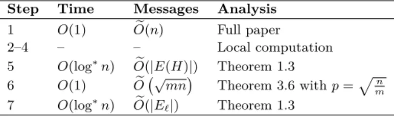
The following theorem summarizes the properties of AlgorithmMST-v1. The running time and message complexity bounds follow from Table 1.
Algorithm 1MST-v1
Input: An edge-weightedn-node,m-edge graphG= (V, E, w).
.Each node knows weights and end-points of incident edges. Every weight can be represented usingO(logn) bits.
Output: An MSTT ofG.
.Each node inV knows which of its incident edges are part ofT. .Letv∗ denote the node with lowest ID inV, known to all nodes.
1: v∗ generates a sequenceπof Θ(log2n) bits independently and uniformly at random and shares with all nodes in V.
2: p←pn m
3: Each node constructs an Θ(logn)-wise-independent sampler from π and uses this to sample each incident edge inGwith probabilityp
4: H ←the spanning subgraph ofGinduced by the sampled edges
5: F ←LinearMessages-MST(H)
6: E`←Compute-F-Light(G, F, p)
7: T ←LinearMessages-MST((V, E`, w))
8: returnT
Table 1Time and message complexity for steps in Algorithm 1MST-v1. Step Time Messages Analysis
1 O(1) Oe(n) Full paper 2–4 – – Local computation 5 O(log∗n) Oe(|E(H)|) Theorem 1.3 6 O(1) Oe √ mn Theorem 3.6 withp=pn m 7 O(log∗n) Oe(|E`|) Theorem 1.3
ITheorem 2.2. Algorithm MST-v1 computes an MST of an edge-weighted n-node, m -edge graph Gwhen it terminates. Moreover, it terminates in O(log∗n)rounds and requires
e
O(√mn)messages w.h.p.
2.2
Trading messages and time
TheMST-v2algorithm (shown in Algorithm 2) is a recursive version ofMST-v1algorithm yielding a time-message trade-off. The algorithm recurses until the number of edges in the subproblem becomes “low” enough to solve it via a call to the LinearMessages-MST subroutine. Specifically, we treat an-node graph withm=O(n1+ε) edges as a base case. For graphs with more edges we use a sampling probability ofp= 1/nε, leading to a sparse graph H with O(m/nε) edges w.h.p., which is recursively processed. The use of limited independence sampling is critical here. One simple approach to sampling an edge would be to let the endpoint with higher ID sample the edge and inform the other endpointif the outcome is positive. Unfortunately, this would lead to the use ofO(m/ne ε) messages w.h.p.,
exceeding our target ofO(ne 1+ε) messages whenmis large3. Using Θ(logn)-wise-independent
sampling allows us to complete the sampling step usingO(n) messages.e
3 This approach would have worked fine for
MST-v1, but to keep the two algorithms consistent to the extent possible, we use the Θ(logn)-wise independent sampler there as well.
Algorithm 2 MST-v2
Input: An edge-weightedn-node,m-edge graph G= (V, E, w)
.Each node knows weights and end-points of incident edges inG. Every weight can be represented usingO(logn) bits. There is a parameter 0< ε≤1, known to all nodes.
Output: An MSTT ofG.
. Each node inV knows which of its incident edges are part ofT. . Letv∗ denote the node with lowest ID in V andc≥1 is a constant.
1: if m < c·n1+εthen
2: T ←LinearMessages-MST(G)
3: returnT
4: else
5: v∗ generates a sequenceπof Θ(log2n) bits independently and uniformly at random and shares with all nodes in V
6: p←1/nε
7: Each node constructs an Θ(logn)-wise-independent sampler fromπand uses this to sample each incident edge inGwith probabilityp
8: H ←the spanning subgraph ofGinduced by the sampled edges
9: F ←MST-v2(H)
10: E`←Compute-F-Light(G, F, p)
11: T ←LinearMessages-MST((V, E`, w))
12: returnT
ITheorem 2.3. Algorithm MST-v2outputs an MST of an edge-weightedn-node,m-edge graph when terminates. Moreover, for anyε >0, it terminates afterO(log∗n/ε)rounds and uses O ne 1+ε/ε
messages, w.h.p.
Proof. If m = O(n1+ε) then the claim follows from Theorem 1.3. Let T(m) denote the time required for Algorithm 2 to compute an MST of a n-node, m-edge graph. Since
Compute-F-Light(·) runs inO(1) time andLinearMessages-MST(·) runs inO(log∗n)
time, we see that, T(m) =T(m/nε) +O(log∗n), for all largem. The first quantity is the
result of a recursive call on the sampled graphH, where each edge is sampled with probability p= 1/nε. Solving this recursion with base casem=O(n1+ε), we getT(m) =O(log∗n/ε).
The message complexity bound is obtained by similar arguments. J Setting ε= log logn/logn, we get the following result.
ICorollary 2.4. There exists an algorithm that computes an MST of ann-node, m-edge input graph and w.h.p. terminates inO(logn·log∗n/log logn) rounds andO(n)e messages.
3
Efficient Computation of
F
-light Edges
In this section we describe theCompute-F-Lightalgorithm and prove its correctness and analyze its time and message complexity. The inputs to this algorithm are the graphG, a spanning forest F of G, and a probability p. Recall that F is the maximal minimum weight spanning forest of the subgraphH obtained by sampling edges inGwith probability p, using a Θ(logn)-wise-independent sampler. The main ideas inCompute-F-Lighthave been informally described in Section 1.2. TheCompute-F-Light algorithm is described below in Algorithm 3.
Algorithm 3Compute-F-Light
Input: (i) An edge-weightedn-node,m-edge graphG= (V, E, w), (ii) A spanning forest F ofG, and (iii) a numberp, 0< p <1.
. F is a maximal minimum weight spanning forest of a subgraphH ofG, whereH is a spanning subgraph ofGobtained by sampling each edge inGwith probability p using a Θ(logn)-wise-independent sampler. Each node knows weights and end-points of incident edges from Gand F. Every weight can be represented usingO(logn) bits.
Output: F-light edges of G.
.Each node inV knows which of its incident edges fromGareF-light.
1: Let {v1, v2, . . . , vc} be set ofcommander nodes (or in short, commanders) wherec = Θ(logn). GatherF at each of these commanders.
2: Each commander simulates Bor˘uvka’s algorithm locally on input graph F. Let Ci = {Ci
1, C2i, . . .} be the set of components at the beginning of Phasei. The node with smallest ID in a component Cji is the leader of component Cji and the ID of the leader serves as the label of each component. For each component Ci
j ∈ Ci, the algorithm picks a MWOE ei
j from F. Components are merged and we get a new set of components Ci+1. If there is no incident edge on a componentCi
j inF then commander setsei
j =⊥with the understanding thatw(⊥) =∞.
3: For each componentCji, commandervi sends the following 3-tuple to each node inCji: (a) Phase numberi, (b) label of Ci
j, and (c)w(eij).
4: A nodev having received a 3-tuple (i, `, w0) associated with component Cji for some i and j computes Θlogp5ndifferent graph sketches with respect to itsw0-restricted neighborhoodNw0(v).
5: The component leader ofCi
j for eachiandj, gathers Θ
log5n p w(ei j)-restricted sketches from all the nodes inCjiand computesw(eij)-restricted sketches ofCji. Then it samples an edge from each sketch computed and notifies the end-points of all sampled edges.
6: returnUnion of sampled edges over alliover allj.
3.1
Analysis
LetCi ={Ci
1, C2i, . . .} be the set of components at the beginning of Phase iof Bor˘uvka’s algorithm being locally simulated onF. Consider the set of edges fromGwith exactly one endpoint inCi
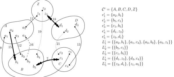
jwith weight at mostw(eij): Lij ={e={u, v} ∈E|u∈Cji, v /∈Cji andw(e)≤ w(eij)}. For example, see Figure 1.
Our first task is to bound the size ofLi
j and for this we appeal to the following lemma from Pettie and Ramachandran [31] on sampling from an ordered set.
ILemma 3.1 (Pettie & Ramachandran [31]). Let χ be a set ofntotally ordered elements and χp be a subset of χ, derived by sampling each element with probabilitypusing ak
-wise-independent sampler. Let Z be the number of unsampled elements less than the smallest element in χp. Then E[Z]≤p−1(8(π/e)2+ 1)fork≥4.
Observe that a straight-forward application of the above lemma gives usE[|Li
j|] =O(1/p). In the next lemma, we modify the proof of Lemma 3.1 in Pettie & Ramachandran [31] to obtain a bound on size ofLij that holds w.h.p.
ILemma 3.2. Pr There exist iandj: |Li
j|> c·log 3
A B C D Z a1 a2 a3 a4 a5 b1 b2 b3 b4 b5 c1 c2 c3 c4 d1 d2 d3 z1 z2 z3 9 15 12 16 11 19 18 21 13 7 Ci={A, B, C, D, Z} ei 1={a2, b1} ei 2={b5, c1} ei 3={c1, b5} ei 4={d1, z3} ei 5={z3, d1} Li 1={{a2, b1},{a1, c3},{a3, b2},{a5, z1}} Li 2={{b5, c1}} Li 3={{c1, b5}} Li 4={{d1, z3},{d3, c4}} Li 5={{z3, d1},{z1, a5}}
Figure 1Illustration of notation and terminology used in Algorithm 3Compute-F-Light. At the beginning of Phaseiof Bor˘uvka’s algorithm, there are 5 components{A, B, C, D, Z}. Each component’s MWOE inF is shown as thick directed arc. Solid arcs show edges inGthat are in respectiveLij’s and hence identified as beingF-light. Dashed arcs (e.g.,a4b3) represent edges that
the algorithm ignores; these edge are notF-light. Dotted arcs (e.g.,b4z2, c2d2) represent edges in
Gwhose status has not yet been resolved by the algorithm. After the merging of components is completed, we end up with two components{ABC, DZ}.
Proof. Fix a Phase i and a component Ci
j in that phase. Let X be the set of all edges fromGhaving exactly one endpoint inCi
j. LetXtbe an indicator random variable defined as Xt = 1 if the tth smallest edge in X is sampled, and 0 otherwise. For any integer `, 1≤`≤ |X|, letS`=P
`
t=1Xtcount the number of ones inX1, . . . , X`. Note thatLij⊆X is a set of all edges with weight at mosteij, the MWOE fromCji inF. This implies that the lightest edge inX that is sampled isei
j, otherwise Bor˘uvka’s algorithm would have chosen a different MWOE. In other words,Xk= 0 for allk≤` if the rank ofeij in the ordered setX is`+ 1 or more. Therefore, Pr |Li
j|> `
=P r(S`= 0).
Observe that,S`is a sum of 0-1 random variables which are Θ(logn)-wise-independent and
E[S`] =p`. By Theorem 1.2, we have Pr(S`= 0)< n13 for` > c·log
3n/pfor some constant c >1. The lemma follows by applying union bound over all phases and components. J ILemma 3.3. For any Phaseiand any component-MWOE pair(Ci
j, eij), w.h.p. O log 5n/p
w(eij)-restricted sketches ofCji are sufficient to find all edges in Lij.
Proof. Consider an oracle which when queried returns an edge in Li
j independently and uniformly at random. LetTs denote the number of the oracle queries required to obtain s=|Li
j|distinct edges (i.e., all edges inLij). Then by the Coupon Collector argument [25], P r(Ts> βslogs)< s−β+1 for anyβ >1. Also, if the oracle is not uniform, but is “almost uniform,” returning an edge in Lij with probability 1s±s−α for a constantα >2, then we getP r(Ts> βslogs+o(1))< s−β+1.
Now, to simulate atthoracle query (t∈[1, T
s]) mentioned above, we sample an unused sketch ofCi
j until we get an edge. Since sampling from a sketch fails with probability at most n−2, w.h.p.,O(1) sketches are sufficient to simulate one oracle query. Hence w.h.p., O(Ts) sketches are sufficient to simulateTsoracle queries. Therefore, with probability at least 1−s−β+1,O(βslogs) sketches are sufficient to getsdistinct edges fromLij.
By Lemma 3.2, we have w.h.p., s = |Li
j| = O log 3
n/p. Therefore by letting s = Θ log3n/p
and β = O(logn) in the above argument, w.h.p., O log5n/p
sketches are sufficient to find all edges inLi
j. J
ILemma 3.4. Let E` be the set ofF-light edges inG. LetL=∪i∪jLij. Then,E`=L. Proof. We first show that L ⊆ E`. Consider a Phase i and a component-MWOE pair (Cji, eij). Consider any edgee={u, v} ∈Lij withu∈Cji, v /∈Cji. Since eij is the MWOE
fromCi
j andu∈Cji, any path inF connectinguto any nodex /∈Cji has to go through edge ei
j. Therefore, for anyx /∈Cji, wF(u, x)≥w(eij). Sincev /∈Cji we havewF(u, v)≥w(eij). Moreover, sincee∈Li
j, we havew(e)≤w(eij) impliesw(e)≤wF(u, v). Hence,eisF-light. Since this is true for anye∈Li
j, we haveLij⊆E`. Hence,L⊆E`.
Now, we show that E` ⊆ L. For any node u ∈ V, let Cq(u) denote the component containingujust before Phaseqof Bor˘uvka’s algorithm (Step 2 in Algorithm
Compute-F-Light). For the sake of contradiction, let there be an edgee={u, v} ∈E`\L. Leti be the index of the phase in which component ofuand component ofv is merged together4 (that is, for anyq < i+ 1,Cq(u)6=Cq(v) andCi+1(u) =Ci+1(v)). Consider the path F(u, v) and note that sinceCi+1(u) =Ci+1(v), the entire pathF(u, v) is inCi+1(u). Now consider the Phasei componentsCi
1, . . . , Cti, t≥2 along this pathF(u, v) (see Figure 2). WLOG, let u∈Ci
1 andv ∈Cti and suppose that the pathF(u, v) visits the components in the order u∈Ci
1, C2i, . . . , Cti−1, v ∈Cti. For example, in Figure 2 the path F(u, v) starts inC1i then goes throughC2i, then toC3i, and finally toC4i. LetF0(u, v) denote the subset of edges in F(u, v) that have endpoints in two distinct Phaseicomponents.
Now consider the MWOE’s of these components: eij is the MWOE forCjiforj= 1,2, . . . , t. There are three cases depending on how the MWOEsei
j relate to the pathF(u, v). ei
j connectsCji toCji+1 for j = 1,2, . . . , t−1. Sincee has exactly one endpoint inC1i ande /∈Li
1 (sincee /∈L), we havew(e)> w(ei1). Furthermore, due to the structure of the MWOEs: w(ei
1)> w(ei2)>· · ·> w(eit−1). This implies thatw(e) is larger than the weights of all edges in F0(u, v).
ei
jconnectsCji toCji−1forj= 2, . . . , t. Sinceehas exactly one endpoint inCtiande /∈Lit (sincee /∈L), we havew(e)> w(ei
t). Furthermore, due to the structure of the MWOEs: w(ei
t)> w(eit−1)>· · ·> w(ei2). This implies thatw(e) is larger than the weights of all edges inF0(u, v).
There is some `, 1≤` < tsuch thatei
j connectsCji toCji+1 for j = 1,2, . . . , ` andeij connectsCji to Cji−1 forj=`+ 1, . . . , t. This case is illustrated in Figure 2 with `= 2. In this case,w(e)> w(ei
1) andw(e)> w(eit) for reasons mentioned in the previous two cases. Furthermore, due to the structure of the MWOEs: w(ei
1)> w(ei2)>· · ·> w(ei`) andw(ei
t)> w(eit−1)>· · ·> w(ei`+1). This implies thatw(e) is larger than the weights of all edges inF0(u, v).
Thus in all three cases, w(e) is larger than the weights of all edges inF0(u, v). Now let eF = {u0, v0} ∈ F be the maximum weight edge in F(u, v). Since e is F-light, we have w(e)< w(eF). This inequality combined with the fact thatw(e) is larger than the weights of all edges inF0(u, v) implies thatu0 andv0 belong to the same Phasei component, i.e., Ci(u0) =Ci(v0). For example, in Figure 2,u0 andv0 are in C2i.
Let Ci(u0) = Ci(v0) = Ci
` for some ` ≤t. LetF(u, v) = F(u, u
0)∪ {u0, v0} ∪F(v0, v).
SinceeF is the heaviest edge inF(u, v), all the edges inF(u, u0) are lighter thaneF. Hence
4 If uand v are never merged into one component, i.e., they are in different components inF then
{u, v} ∈Lijwhereiis the phase in whichu’s component becomes maximal with respect toF andjis such thatubelongs toCji. This follows from the fact thateij=⊥andw(eij) =∞.
u e v ei 1 ei 2 ei 3 ei 4 eF Ci 2 C3i Ci 4 Ci 1 u0 v0
Figure 2Illustration of proof of Lemma 3.4. After Phasei, componentsC1i, C2i, C3i, C4iare merged
together using edgesei1, ei2, e3i, ei4inF. Dashed curves represent paths inF between the respective
end-points. eis anF-light edge. eF is the heaviest edge on path fromutovinF.
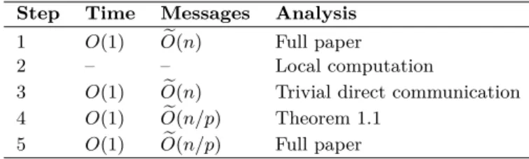
Table 2Time and message complexity for steps in Algorithm 3Compute-F-Light. Step Time Messages Analysis
1 O(1) Oe(n) Full paper
2 – – Local computation
3 O(1) Oe(n) Trivial direct communication
4 O(1) Oe(n/p) Theorem 1.1
5 O(1) Oe(n/p) Full paper
at any Phase i0< i, Bor˘uvka’s algorithm considers edges inF(u, u0) for componentCi0(u0) and edges inF(v0, v) for componentCi0(v0) before consideringe
F. The implication of this is, Ci(u) =Ci(u0) andCi(v) =Ci(v0). But, Ci(u)6=Ci(v) therefore, Ci(u0)6=Ci(v0) – a
contradiction. J
From Lemma 3.2 and Lemma 3.4 we get the following bound on the number ofF-light edges inG.
ICorollary 3.5. W.h.p., the number of F-light edges inGis Oe(n/p).
Table 2 summarizes the time and message complexity of each step of Algorithm Compute-F-Light. A naive implementation of Step 5 may require super-constant number of rounds because of receiver-side bottlenecks, but a more sophisticated implementation that appears in the full version of the paper [30] shows how to implement this step inO(1) rounds, using
e
O(n/p) messages.
From Lemma 3.4 and Table 2 we get the following result.
ITheorem 3.6. Algorithm Compute-F-Light computes allF-light edges for given graph
Gand a minimum spanning forest F of H where H is obtained by sampling each edge in
Gwith probability pusing aΘ(logn)-wise-independent sampler. Moreover, the computation takes O(1)rounds and usesOe(n/p)messages w.h.p.
References
1 Kook Jin Ahn, Sudipto Guha, and Andrew McGregor. Analyzing graph structure via linear measurements. In Proceedings of the 23rd annual ACM-SIAM Symposium on Discrete Algorithms (SODA), pages 459–467, 2012.
2 Kook Jin Ahn, Sudipto Guha, and Andrew McGregor. Graph sketches: sparsification, spanners, and subgraphs. InProceedings of the 31st Symposium on Principles of Database Systems (PODS), pages 5–14, 2012.
3 Andrew Berns, James Hegeman, and Sriram V. Pemmaraju. Super-Fast Distributed Algo-rithms for Metric Facility Location. InProccedings of the 39th International Colloquium on Automata, Languages, and Programming (ICALP), pages 428–439, 2012.
4 Keren Censor-Hillel, Petteri Kaski, Janne H. Korhonen, Christoph Lenzen, Ami Paz, and Jukka Suomela. Algebraic methods in the congested clique. In Chryssis Georgiou and Paul G. Spirakis, editors,Proceedings of the 2015 ACM Symposium on Principles of Dis-tributed Computing, PODC 2015, Donostia-San Sebastián, Spain, July 21-23, 2015, pages 143–152. ACM, 2015. doi:10.1145/2767386.2767414.
5 Graham Cormode and Donatella Firmani. A unifying framework for`0-sampling algorithms.
Distributed and Parallel Databases, 32(3):315–335, 2014.
6 Danny Dolev, Christoph Lenzen, and Shir Peled. “Tri, Tri Again”: Finding Triangles and Small Subgraphs in a Distributed Setting. In Proceedings of the 26th International Symposium on Distributed Computing (DISC), pages 195–209, 2012.
7 Andrew Drucker, Fabian Kuhn, and Rotem Oshman. The communication complexity of distributed task allocation. InProceedings of the 30st ACM Symposium on Principles of Distributed Computing (PODC), pages 67–76, 2012. doi:10.1145/2332432.2332443. 8 Michael Elkin. An Unconditional Lower Bound on the Time-Approximation Trade-off for
the Distributed Minimum Spanning Tree Problem.SIAM J. Comput., 36(2):433–456, 2006. doi:10.1137/S0097539704441058.
9 Joachim Gehweiler, Christiane Lammersen, and Christian Sohler. A Distributed O(1)-approximation Algorithm for the Uniform Facility Location Problem. In Proceedings of the 18th Annual ACM Symposium on Parallelism in Algorithms and Architectures (SPAA), pages 237–243, 2006. doi:10.1145/1148109.1148152.
10 Mohsen Ghaffari and Merav Parter. MST in Log-Star Rounds of Congested Clique. InProc. of the 2016 ACM Symposium on Principles of Distributed Computing, PODC’16, 2016. 11 James W. Hegeman, Gopal Pandurangan, Sriram V. Pemmaraju, Vivek B. Sardeshmukh,
and Michele Scquizzato. Toward Optimal Bounds in the Congested Clique: Graph Connec-tivity and MST. InProceedings of the 2015 ACM Symposium on Principles of Distributed Computing, PODC’15, pages 91–100. ACM, 2015. doi:10.1145/2767386.2767434. 12 James W. Hegeman and Sriram V. Pemmaraju. Lessons from the Congested Clique
Applied to MapReduce. In Proceedings of the 21th International Colloquium on Struc-tural Information and Communication Complexity (SIROCCO), pages 149–164, 2014. doi:10.1007/978-3-319-09620-9_13.
13 James W. Hegeman, Sriram V. Pemmaraju, and Vivek B. Sardeshmukh. Near-Constant-Time Distributed Algorithms on a Congested Clique. In Proceedings of the 28th Interna-tional Symposium on Distributed Computing (DISC), pages 514–530, 2014.
14 Stephan Holzer and Nathan Pinsker. Approximation of Distances and Shortest Paths in the Broadcast Congest Clique. CoRR, abs/1412.3445, 2014.
15 Hossein Jowhari, Mert Sağlam, and Gábor Tardos. Tight Bounds for Lp Samplers, Find-ing Duplicates in Streams, and Related Problems. InProceedings of the Thirtieth ACM SIGMOD-SIGACT-SIGART Symposium on Principles of Database Systems, PODS’11, pages 49–58. ACM, 2011. doi:10.1145/1989284.1989289.
16 David R. Karger, Philip N. Klein, and Robert E. Tarjan. A Randomized Linear-time Algorithm to Find Minimum Spanning Trees. J. ACM, 42(2):321–328, March 1995. doi: 10.1145/201019.201022.
17 Valerie King, Shay Kutten, and Mikkel Thorup. Construction and impromptu repair of an mst in a distributed network with o(m) communication. InProceedings of the 2015 ACM
Symposium on Principles of Distributed Computing, PODC’15, pages 71–80, New York, NY, USA, 2015. ACM. doi:10.1145/2767386.2767405.
18 Hartmut Klauck, Danupon Nanongkai, Gopal Pandurangan, and Peter Robinson. Dis-tributed Computation of Large-Scale Graph Problems. InProceedings of the 26th Annual ACM-SIAM Symposium on Discrete Algorithms (SODA), pages 391–410, 2015.
19 Janne H. Korhonen. Deterministic MST sparsification in the congested clique. CoRR, abs/1605.02022, 2016. URL:http://arxiv.org/abs/1605.02022.
20 Shay Kutten, Gopal Pandurangan, David Peleg, Peter Robinson, and Amitabh Trehan. On the complexity of universal leader election. J. ACM, 62(1):7:1–7:27, March 2015. doi: 10.1145/2699440.
21 Shay Kutten and David Peleg. Fast Distributed Construction of Smallk-Dominating Sets and Applications. J. Algorithms, 28(1):40–66, 1998. doi:10.1006/jagm.1998.0929. 22 Christoph Lenzen. Optimal Deterministic Routing and Sorting on the Congested Clique. In
Proceedings of the 31st ACM Symposium on Principles of Distributed Computing (PODC), pages 42–50. ACM, 2013. doi:10.1145/2484239.2501983.
23 Zvi Lotker, Boaz Patt-Shamir, Elan Pavlov, and David Peleg. Minimum-Weight Spanning Tree Construction inO(log logn) Communication Rounds. SIAM Journal on Computing, 35(1):120–131, 2005.
24 Andrew McGregor. Graph stream algorithms: A survey. ACM SIGMOD Record, 43(1):9– 20, 2014.
25 Rajeev Motwani and Prabhakar Raghavan.Randomized Algorithms. Cambridge University Press, New York, NY, USA, 1995.
26 Danupon Nanongkai. Distributed approximation algorithms for weighted shortest paths. InProc. of the 46th ACM Symp. on Theory of Computing (STOC), pages 565–573, 2014. 27 Gopal Pandurangan, Peter Robinson, and Michele Scquizzato. A time- and message-optimal
distributed algorithm for minimum spanning trees. CoRR, abs/1607.06883, 2016. URL: http://arxiv.org/abs/1607.06883.
28 Boaz Patt-Shamir and Marat Teplitsky. The Round Complexity of Distributed Sorting. In
Proceedings of the 30th Annual ACM Symposium on Principles of Distributed Computing (PODC), pages 249–256, 2011. doi:10.1145/1993806.1993851.
29 David Peleg. Distributed Computing: A Locality-Sensitive Approach. Society for Industrial Mathematics, 2000.
30 Sriram V. Pemmaraju and Vivek B. Sardeshmukh. Super-fast MST algorithms in the congested clique usingo(m) messages. CoRR, abs/1610.03897, 2016. URL:http://arxiv. org/abs/1610.03897.
31 Seth Pettie and Vijaya Ramachandran. Randomized minimum spanning tree algorithms using exponentially fewer random bits. ACM Trans. Algorithms, 4(1), 2008.doi:10.1145/ 1328911.1328916.
32 Atish Das Sarma, Stephan Holzer, Liah Kor, Amos Korman, Danupon Nanongkai, Gopal Pandurangan, David Peleg, and Roger Wattenhofer. Distributed Verification and Hardness of Distributed Approximation. SIAM J. Comput., 41(5):1235–1265, 2012.
33 Jeanette P. Schmidt, Alan Siegel, and Srinivasan Aravind. Chernoff-Hoeffding Bounds for Applications with Limited Independence. SIAM J. Discrete Math., 8(2):223–250, 1995. doi:10.1137/S089548019223872X.
34 Robert Endre Tarjan. CBMS-NSF Regional Conference Series in Applied Mathematics: Data Structures and Network Algorithms. Society for Industrial and Applied Mathematics, New York, NY, USA, 1983.