Full Length Review Article
PERFORMANCE STUDY AND THERMAL PROFILE CHARACTERIZATION OF LOW TEMPERATURE
VISCOSITY BATH IN DIFFERENT TEMPERATURE RANGES
*Mohy, E., Mekkawy, M. M. and Abu-Dorra, H. M.
National Institute for Standards, Tersa St., El Haram, Giza 12211, Egypt
ARTICLE INFO ABSTRACT
A new Viscosity bath has been entered the services in Thermal Metrology Laboratory-National Institute for Standards, NIS-Egypt in order to use in maintain and extend the national viscosity scale in wide temperature ranges, international comparison and routine calibration of viscometers. The medium of the bath should be homogenous enough in temperature so many thermal factors taken into account to estimate the temperature gradient, homogeneity, stability and thermal profile distribution with the related uncertainty to each parameter. The study carried out by two Standards Platinum Resistance Thermometer (SPRT) calibrated at fixed point according to ITS-90.
Copyright © 2015 Mohy et al. This is an open access article distributed under the Creative Commons Attribution License, which permits unrestricted use, distribution, and reproduction in any medium, provided the original work is properly cited.
INTRODUCATION
Viscosity laboratory decided to extend the national viscosity scale in low temperature range down to -30oC, new viscosity bath works with low temperature range using dry denatured ethanol is used as the bath medium because its property to absorb moisture from the atmosphere is removed from it. The oil bath model Koehler LKV4000 low temperature kinematic viscosity bath contains several upper holes to receive four viscometers at the same time, there isan additional small hole to insert the Standard Platinum Resistance Thermometers (SPRTs) to measure the temperature variation during the viscosity measurements. The cooling unit within the bath
stabilize the bath temperature to desired setting within
± 0.02⁰C. The bath is filled with approximately 14L of ethanol
as a medium to put inside it the viscometers in order to calibrate glass viscometer under test with references known oils or even known viscometers with unknown oils under test. the main target is realize the kinematic viscosity tests with glass capillary viscometers according to the ASTM D445 (ASTM, 1992) test method and related test specifications. The SPRTs SN 234, 247 has been calibrated at fixed point according to ITS-90 (Preston-Thomas, 1990).
*Corresponding author: Mohy, E., National Institute for Standards, Tersa St., El Haram, Giza 12211, Egypt
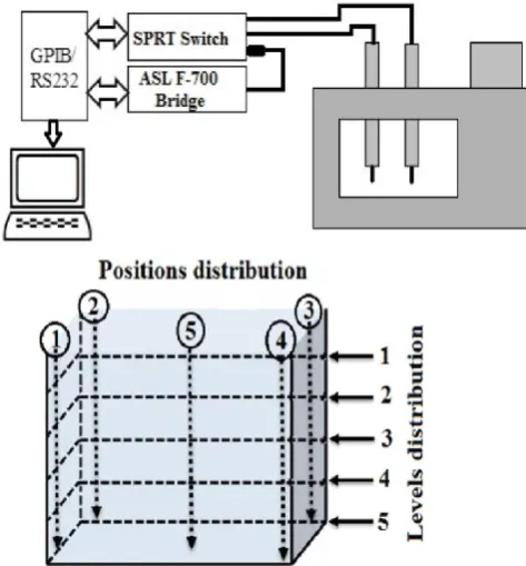
Experimental arrangement
The bath filed with 14L of ethanol then the SPRTs have been inserted into the medium at different positions and levels. Five levels taken into the account from the top side down to the bottom separate equally from each other’s, at each level the thermometer inserted in five positions as four at the corners and one at the center of the level as shown in Figure 1. So, twenty five position introduced into the study at each
temperature set point, the range of interest is from -30 oC up to
10 oC. The measurements carried out at -30oC, -20oC, -10 oC
and 10 oC. The two SPRT connected at the same time to
resistance bridge model ASL F700 conjugated with standard resistor and the measuring system connected to PC working under LABVIEW environment.
Metrological Characterizations
Homogeneity is the main parameter should be studied to optimize and establish a suitable uniform medium realize the National Viscosity Scale. In order to find a closed value to the homogeneity as possible, thermal gradient taken into account and observed as a change of a temperature readings of a thermometer according to a change of its position inside a calibration bath (Pornpatkul, 2012). Basic gradients that can
ISSN: 2230-9926
International Journal of Development Research
Vol. 5, Issue, 02, pp. 3317-3321, February,2015
DEVELOPMENT RESEARCH
Article History:
Received 22nd November, 2014
Received in revised form 28th December, 2014
Accepted 15th January, 2015
Published online 27th February, 2015
be observed are vertical and horizontal gradient but sometimes more appropriate to define axial and a radial gradient.
[image:2.595.315.539.254.657.2]Figure 1. Schematic diagram of levels and position distribution
Table 1. Temperature distribution measurements using SPRT SN 234
L Temperature〈 〉*
SPRT 234
1 P T -30.00 -20.00 -10.00 10.00
1 〈 〉 -30.00138 -20.02123 -10.02138 10.02811
2 〈 〉 -30.00149 -20.02127 -10.02154 10.02823
3 〈 〉 -30.00152 -20.02129 -10.02167 10.02841
4 〈 〉 -30.00144 -20.02139 -10.02172 10.02852
5 〈 〉 -30.00131 -20.02156 -10.02183 10.02857
2 P T -30.00 -20.00 -10.00 10.00
1 〈 〉 -30.00121 -20.02134 -10.02136 10.02822
2 〈 〉 -30.00124 -20.02156 -10.02176 10.02847
3 〈 〉 -30.00157 -20.02144 -10.02149 10.02833
4 〈 〉 -30.00156 -20.02165 -10.02159 10.028342
5 〈 〉 -30.00192 -20.02154 -10.02158 10.02897
3 P T -30.00 -20.00 -10.00 10.00
1 〈 〉 -30.00198 -20.02183 -10.02222 10.02865
2 〈 〉 -30.00204 -20.02194 -10.02234 10.02860
3 〈 〉 -30.00213 -20.02211 -10.02256 10.02880
4 〈 〉 -30.00209 -20.02256 -10.02277 10.02832
5 〈 〉 -30.00221 -20.02252 -10.02281 10.02854
4 P T -30.00 -20.00 -10.00 10.00
1 〈 〉 -30.00202 -20.02238 -10.02321 10.02910
2 〈 〉 -30.00218 -20.02241 -10.02333 10.02930
3 〈 〉 -30.00232 -20.02244 -10.02345 10.02949
4 〈 〉 -30.00241 -20.02253 -10.02377 10.02961
5 〈 〉 -30.00221 -20.02259 -10.02281 10.02983
5 P T -30.00 -20.00 -10.00 10.00
1 〈 〉 -30.00265 -20.02244 -10.02312 10.03017
2 〈 〉 -30.00273 -20.02257 -10.02319 10.03032
3 〈 〉 -30.00279 -20.02269 -10.02341 10.03048
4 〈 〉 -30.00281 -20.02274 -10.02369 10.03069
5 〈 〉 -30.00280 -20.02272 -10.02389 10.03083
Uncertainty contribution of an axial gradient is determined as maximum temperature difference between two different positions in axial direction. The radial gradient is a maximum temperature difference between two different positions in a radial direction. So, three thermal factors were discussed as follows;
Thermal profile distribution
Consider that the temperature denotes to the temperature
at level Lx and position Py, the two SPRT measure the temperature at different positions and levels as shown in Table 1 and 2.
Table 2. Temperature distribution measurements using SPRT SN 247
L Temperature〈 〉 SPRT 247
1 P T -30.00 -20.00 -10.00 10.00
1 〈 〉 -30.00184 -20.02176 -10.02196 10.02844
2 〈 〉 -30.00190 -20.02182 -10.02178 10.02867
3 〈 〉 -30.00201 -20.02174 -10.02181 10.02843
4 〈 〉 -30.00199 -20.02191 -10.02190 10.02887
5 〈 〉 -30.00188 -20.02185 -10.02198 10.02889
2 P T -30.00 -20.00 -10.00 10.00
1 〈 〉 -30.00170 -20.02158 -10.02176 10.02860
2 〈 〉 -30.00178 -20.02174 -10.02181 10.02866
3 〈 〉 -30.00198 -20.02179 -10.02189 10.02895
4 〈 〉 -30.00192 -20.02168 -10.02197 10.02887
5 〈 〉 -30.00197 -20.02194 -10.02191 10.02893
3 P T -30.00 -20.00 -10.00 10.00
1 〈 〉 -30.00214 -20.02196 -10.02285 10.02897
2 〈 〉 -30.00243 -20.02218 -10.02239 10.02914
3 〈 〉 -30.00258 -20.02254 -10.02263 10.02945
4 〈 〉 -30.00278 -20.02279 -10.02279 10.02976
5 〈 〉 -30.00292 -20.02289 -10.02289 10.028
983
4 P T -30.00 -20.00 -10.00 10.00
1 〈 〉 -30.00219 -20.02213 -10.02253 10.02945
2 〈 〉 -30.00234 -20.02229 -10.02274 10.02968
3 〈 〉 -30.00256 -20.02237 -10.02281 10.02979
4 〈 〉 -30.00289 -20.02259 -10.02289 10.02987
5 〈 〉 -30.00299 -20.02287 -10.02292 10.02999
5 P T -30.00 -20.00 -10.00 10.00
1 〈 〉 -30.00398 -20.02368 -10.02389 10.03633
2 〈 〉 -30.00421 -20.02382 -10.02417 10.03651
3 〈 〉 -30.00437 -20.02397 -10.02444 10.03723
4 〈 〉 -30.00461 -20.02418 -10.02464 10.03820
5 〈 〉 -30.00482 -20.02479 -10.02492 10.03915
*<> brackets indicates to the average
Temperature Stability
The stability of the bath shows lower variation within the regulation specification of the bath. The fluctuation was
monitored at different positions and levels as shown in
Figure 2 for SPRT SN-234 at setting point -10.0oC. The
[image:2.595.39.279.388.767.2]=(∆ ∆ ) (1)
During the progressive study of the performance of the Bath, it
[image:3.595.312.554.49.192.2]is found that the stability was better than 0.015oC.
Figure 2. Temperature stability at the center of the bath at -10 oC.
Thermal Gradient
The vertical gradient in a bath is termed “axial uniformity”. The horizontal gradient in a bath is termed “radial uniformity” (EURAMET, 2011).
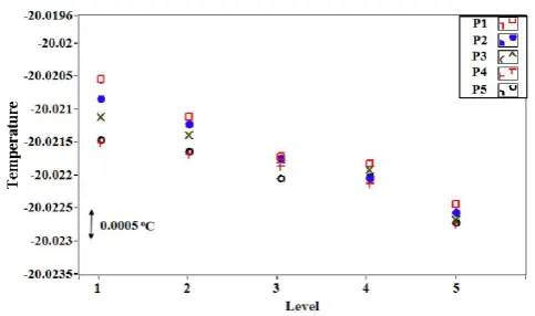
Vertical Thermal Gradient
[image:3.595.41.290.115.265.2]Figures from 3to 10 show the temperature gradient due to thermometer depths through five levels at different setting points for SPRTs SN 234 and SN 247.
[image:3.595.317.551.234.370.2]Figure 3. Thermal axial gradient at -30.0 oC for SPRT SN 234.
Figure 4. Thermal axial gradient at -30.0 oCfor SPRT SN 247.
Figure 5.Thermal axial gradient at -20.0 oC for SPRT SN 234.
[image:3.595.321.549.416.548.2]Figure 6. Thermal axial gradient at -20.0 oC for SPRT SN 247.
Figure 7. Thermal axial gradient at -10.0 oC for SPRT SN 234.
[image:3.595.41.284.572.704.2] [image:3.595.319.548.588.722.2]Figure 9. Thermal axial gradient at 10.0 oC for SPRT SN 234.
Figure 10. Thermal axial gradient at 10.0 oC for SPRT SN 247.
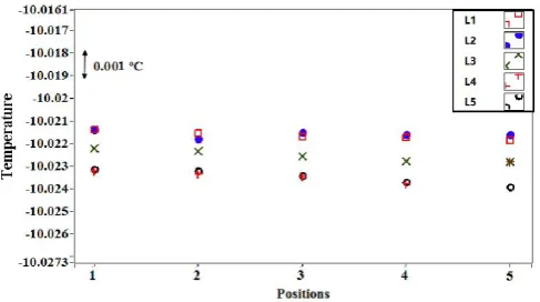
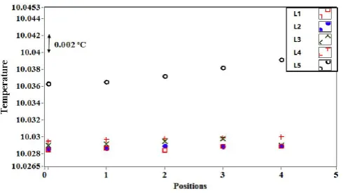
Horizontal Thermal Gradient
[image:4.595.42.281.218.349.2]Figures from 11 to 18 show the temperature gradient due to thermometer positions at each level at different setting points for SPRTs SN 234 and SN 247.
Figure 11. Thermal radial gradient at -30.0 oC for SPRT SN 234.
[image:4.595.310.552.224.356.2]Figure 12. Thermal radial gradient at -30.0 oC for SPRT SN 247.
[image:4.595.310.554.390.526.2]Figure 13. Thermal radial gradient at -20.0 oC for SPRT SN 234.
[image:4.595.309.554.558.693.2]Figure 14. Thermal radial gradient at -20.0 oC for SPRT SN 247.
Figure 15. Thermal radial gradient at -10.0 oC for SPRT SN 234.
[image:4.595.38.286.611.749.2]Figure 17. Thermal radial gradient at 10.0 oC for SPRT SN 234.
Figure 18. Thermal radial gradient at 10.0 oC for SPRT SN 247.
In order to calculated the thermal gradient which define from the following equation
= + +
The study was carried out on two dimensions vertical and horizontal.
The axial thermal gradient = 0.014. The Radial thermal gradient = 0.012.
Uncertainty Estimation
The combined standard uncertainty of a measurement result is taken to represent the estimated standard deviation of the result. It is obtained by combining the individual standard
uncertainties ui, whether arising from Type A and Type B
evaluation (GUM, 1995).
( ) = ∑ ( )(2)
Combined uncertainty calculated from
[image:5.595.40.285.217.355.2]= + + + . + . + .
Table 3. Uncertainty for a metrology bath with a standard thermometer as the readout
Uncertainty Contributors Symbol Uncertainty (°C)
Stability uSt 0.015
Radial uniformity uRa. 0.012
Axial uniformity uAx 0.014
Reference SPRTs calibration certificates uC.C 0.001
Thermometry Bridge uT.B 0.00027
Heat Flux from ambient uH.F 0.0022
Combined Standard Uncertainty (UC) 0.023894
Expanded Uncertainty (k=2) 0.047788
Conclusion
An intensive work was carried out on studying the new metrological viscosity bath to realize the national viscosity scale in wide temperature ranges. The results show that the
bath worked with stability better than 0.015 oC. Thermal
profile distribution achieved by two SPRTs calibrated at ITS-90 to calculate the thermal gradient homogenty. Thermal axial
and radial gradient equivalent to 0.014 oC and 0.012 oC
respectively.
REFERENCES
ASTM D2162, 1992. Basic calibration of master viscometers and viscosity oil standards.
Preston-Thomas, H. 1990. International Temperature
Scale1990 (ITS-90), National Research Council of Canada, Ottawa, KIA OSI, Canada.
Pornpatkul, C. 201. Temperature Sensor Calibration by Liquid Bath Control System, ICEAST 2012, International Conference on Engineering Applied Sciences and Technology, Nov 21-24, Bangkok, Thailand.
Ghazanfar, M. 2013. A Simple Method for the Calibration of an Open Surface Water Bath IOP Conf. Series: Materials
Science and Engineering 51, 012015
doi:10.1088/1757899X/51/1/012015
EURAMET/cg-13/v.2.0, Guide Line to Liquid Calibration Bath, 03/2011.
GUM: Guide to the expression of uncertainty in measurement. BIPM/IEC/IFCC/ISO/OIML/IUPAC, 1995.