Machine learning and statistical analysis in material property prediction

(1)

Copyright by Zhuoya You

(2)

The Report Committee for Zhuoya You

Certifies that this is the approved version of the following Report:

Machine Learning and Statistical Analysis

in Material Property Prediction

APPROVED BY

SUPERVISING COMMITTEE:

Wei Li, Supervisor

(3)

Machine Learning and Statistical Analysis

in Material Property Prediction

by

Zhuoya You

Report

Presented to the Faculty of the Graduate School of The University of Texas at Austin

in Partial Fulfillment of the Requirements

for the Degree of

Master of Science in Engineering

(4)

Abstract

Machine Learning and Statistical Analysis

in Material Property Prediction

Zhuoya You, M.S.E

The University of Texas at Austin, 2018 Supervisor: Wei Li

Abstract: With the development of algorithms, models and data-driven efforts in other areas, machine learning is beginning to make impacts in materials science and engineering. In this work, we review the basic steps of using machine learning in materials science. We also develop several machine learning methods to predict the two physically-distinct properties of transparent conductors: formation enthalpy, which is an indication of stability, and bandgap energy, which is an indication of optical transparency. These include regression-based models such as the ordinary least squares (OLS) regression model, stepwise selection model, Ridge model and Lasso model, and tree-based models such as the random forest model and gradient boosted model (GBM). We discuss the advantages and potential problems of each model and provide suggestions for possible applications.

(5)

Chapter 1: Introduction

Machine learning is an application of artificial intelligence (AI) in the real world. It enables systems and devices to learn automatically and improve the processes and results from past experiences without being explicitly programmed. Machine learning mostly focuses on the development of computer programs which can access input data and use algorithms to predict and forecast output values.

With the development of algorithms, models and data-driven efforts in other areas, machine learning is beginning to make impacts in materials science and engineering. Machine learning methods help provide rapid predictions based on past data rather than direct experimentation or computational simulations. Machine learning is different from the theoretical approach and laboratory experimentation, which are the traditional forms of techniques for materials research and design. Machine learning is a much more efficient approach to accelerating the innovation of materials [4].

In this work, we review the basic steps of using machine learning in materials science. We also developed several machine learning methods to predict the two physically-distinct properties of transparent conductors: formation enthalpy, which is an indication of stability, and bandgap energy, which is an indication of optical transparency. These include regression-based models such as the ordinary least squares (OLS) regression model, stepwise selection model, Ridge model and Lasso model, and tree-based models such as the random forest model and gradient boosted model (GBM). We discuss the advantages and potential problems of each model and provide suggestions for possible applications.

(7)

Chapter 2: Literature Review

Recently, data to result and prediction ideas are beginning to show great effectiveness in the field of materials science and engineering. Generally, the development and innovation of new materials is a costly trial‐and‐error process and takes a long time to conduct. Machine learning as an emerging component of computational science is making significant improvement in both efficiency and prediction accuracy in materials development, promising considerable bright future for materials research and discovery [9]. The institute of Materials Genome Initiative (MGI), which envisions the innovation, manufacturing, and development of advanced materials twice as fast as previously, also emphasized on the need for such advanced data analytics techniques [3].

There are already successful examples making effective use of machine learning in materials research. These examples include using historical data toward fast and accurate predictions of material phase diagrams, applying machine learning models to predict the crystal structure and consequent properties of materials, and developing interatomic potentials and energy functionals to enhance the efficiency and accuracy of materials simulation [6]. For instance, by using the data from the MatNavi database of Japan National Institute of Material Science, Agrawal et al. built successful machine learning models to predict the strength fatigue of steel [1]. Paul et al. developed a predictive analytics framework which embedded machine learning algorithms to perform a quantum mechanical DFT simulation [2]. Through machine learning algorithms and data engineering, Liu et al. conducted microstructure optimization of a magnetoelastic Fe-Ga alloy (Galfenol). The method can also be used to improve properties including elastic, plastic and magnetostrictive performances [11].

(8)

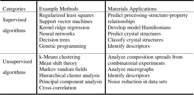
The following Table describes some typical material science applications of different machine learning algorithms [12].

Categories Example Methods Materials Applications Supervised

algorithms

Regularized least squares Support vector machines Kernel ridge regression Neural networks Decision trees Genetic programming

Predict processing-structure-property relationships

Develop model Hamiltonians Predict crystal structures Classify crystal structures Identify descriptors Unsupervised

algorithms

k-Means clustering Mean shift theory Markov random fields Hierarchical cluster analysis Principal component analysis Cross-correlation

Analyze composition spreads from combinatorial experiments

Analyze micrographs Identify descriptors

Noise reduction in data sets

(9)

Chapter 3: Basic Steps of Machine Learning in Materials Science

3.1.DATA PREPARATION

In materials science, the original datasets are usually collected from computational simulations or experimental measurements. These original datasets are often incomplete, noisy, and inconsistent. Thus, data cleaning and pre-processing are important.

3.1.1 Zero-variance predictor detection

In some situations, the data generating mechanism may create predictors that only have one constant value. These predictors are called zero-variance predictor. Such a predictor provides no explanation of the variance of response variables. In many situations, this variable may cause models to crash or the fit to be unable. Thus, these “zero-variance” predictors need to be identified and removed before modeling.

3.1.2 Identifying correlated predictors

A predictor variable may be redundant which means that it “overlaps” with other variables. If some of the predictors or variables in a dataset are highly correlated with others, there is collinearity. High level of correlation between variables can lead to multicollinearity. Multicollinearity will result in serious numerical and statistical difficulties in fitting a regression model. Thus, before a model is built redundant or collinear predictors should be deleted.

3.1.3 Variable transformation

(10)

with a spread equal to 1 or become dimensionless. It is useful for comparing variables with different units. Second, reducing skewness. Usually a symmetric distribution is much easier to deal with and more interpretable than a skewed distribution. Third, obtaining equal spreads. Homoscedastic data is easier to analyze and interpret than heteroscedastic data. Fourth, enhancing linear relationship. Finally, data transformation helps to change to additive relationships. The most often used transformations are the reciprocal, logarithm, cube root, square root, and square of the original data.

3.2MODEL CONSTRUCTION

Depending on the prerequisites and major requirement, usually we will split the cleaned dataset into two parts – the train subset and the test subset. The train sub dataset is used for developing or training the model. The test part is used as a reference to check the validation of the trained model. Model development is essentially a black box, which links input data and output data using a specific set of nonlinear or linear functions. Machine learning methods provide a way to find the coefficients, with which a certain mapping function approximates the target function as closely as possible.

We divide the machine learning models for material properties prediction in this work into two categories: 1) regression based models such as multiple linear regression, logistic regression, ridge regression, artificial neural network, and support vector regression; 2) tree base models such as decision tree, support vector classification, naive Bayes, random forest, and gradient boosted models. Each algorithm has its own scope of application, and thus there is no one algorithm that fits all problems. Model selection is important in material properties prediction.

(11)

3.3MODEL EVALUATION

Model evaluation includes the steps of validating the algorithms through different strategies and analysis of their predictive accuracy by calculating performance metrics. 3.3.1 Model Validation

The validation step is important. It helps to find the best parameters for the model. It also helps to prevent the problem of overfitting. The most commonly used strategies for the validation step are the hold-out strategy, k-fold cross-validation strategy, and bootstrap strategy [5].

In the hold-out strategy, the original dataset is randomly split into two parts. The left-in part is treated as the training set, and the left-out part is treated as validation set or test set. In this strategy, in order to keep the consistency of the data distribution, the sampling method “stratified sampling” is often used. The advantages of this strategy are that it includes the whole independent data and that it is time and cost efficient since it only needs to run once. The disadvantage of this strategy is that since this only run once, the performance valuation is subject to higher variance if the given dataset is small. The validation or test set error may tend to overestimate the test error for the model fit on the entire data set.

The K-fold cross validation strategy evaluates the data across the entire training set. The data set is randomly divided into K equal-sized folds (K-equal subsets) and each time we will leave one subset out and trains the model with the other K-1 folds [17]. Thus, the model will be trained for K times. At the end, the performance metric, such as RMSE for numeric response variables, or ROC for categorical variables is averaged across the K trainings, and through this process the best parameter combination has been

(12)

set is the entire data training. However, this strategy is not cost efficiency if the data set is very large because the model needs to be trained K times at the validation step.

The bootstrap strategy is a flexible and powerful statistical method that often used to quantify the uncertainty which associated with a given estimator or statistical learning method. The bootstrapping strategy create new data sets by sampling the observations from original dataset [16]. By using this strategy, we can get the estimator without obtain new or additional observations from the research population. Every “bootstrap data sets” is created by sampling with replacement, and its sample size of the bootstrap data set are the same as the original dataset, therefore it is very effective when the dataset is small and unable or difficult to get additional sample from the research population. However, the bootstrapping also has shortage, because the bootstrapping process may change the original distribution, so it may introduce estimation bias.

3.3.2 Performance Metrics

To measure predictive performance of different models, we need to summarize the difference between observations and predict value from models by a certain performance metric. The most commonly used metrics for evaluating model performance are the root mean square error (RMSE) and area under the receiver operating curve (AUC).

The root mean square error (RMSE) is given as:

RMSE = √1

n∑(ŷ − yi i)2

n

i=1

where ŷ_iis the estimated value from the model, 𝑦_𝑖 is the observation value, n is the number of samples available. RMSE is an error metric, which means the lower values the

(13)

RMSE, the better predictive performance the model. RMSE is the most used metrics for regression-based model.

Receiver operating curve (ROC) summarizes performance of a binary classification over all possible thresholds. ROC has “false positive rate” on the x-axis and “true positive rate” on the y-axis, each point of the curve corresponds to a choice of a threshold [13]. Area under the ROC curve (AUC) provides a summary performance measure across all possible thresholds. AUC is 1 for a perfect model and 0.5 for random predictions, AUC it is interpreted as a reward, the higher the better. The fundamental difference between RMSE and AUC is that RMSE considers absolute values of predictions, whereas AUC only consider about their relative ordering.

(14)

Chapter 4: Machine Learning Models for Material Property Prediction

4.1REGRESSION BASED MODELS

In this work we introduce four regression-based models including ordinary least squares (OLS) regression models, stepwise selection models, Ridge regression models, and Lasso regression models for material property prediction.

4.1.1 OLS regression model

Ordinary least squares (OLS) or linear least squares regression is the most basic and most commonly used prediction model. OLS is a method for estimating the unknown parameters in a linear regression model by minimizing the sum of the squares of the differences between the observed dependent predictor variable in the given dataset and those predicted by the linear function[14].

If we consider a dataset with N cases (Xi_{, y}

i), i = 1.2, … . . , N, where Xi =

(x_i1,… x_ip)T_{are the predictor variables and} _y

iare the responses. The OLS regression

model can be given by the following function:

y_i = α + β₁x_i1+ β₁₂x_i2+ ⋯ + β_px_ip+ ε_i

Here β_i, i = 1 … p are regression coefficients for each predictor, ε_iis the error term which has a normal distribution with the mean of 0 and variance of σ2_{. The}

regression model can also be written as y_i = β₀− x_iT_{β . And the objective of OLS}

regression is to solve the following function: {1 N β0,β min _{∑ (y} i− β0− xiT N 1 β)2}

OLS regression is sample, easy to interpret and sometimes it is as powerful as many complex models. However, it can cause serious difficulties in dealing with big data set. First, if the data has many independent explanatory variables, OLS regression estimator may not uniquely exist. Second, because the OLS estimates depend

(15)

on (XT_X)−1_{, we would have problems in computing βifX}𝑇_{X, if it is singular or nearly}

singular. In those cases, small changes to the elements of X will lead to large changes in XT_{X. Moreover, OLS regression has the risk of overfitting in some situation, which}

means the least square estimator β may provide a good fit to the training data, but it will give a disastrous prediction for the test data. To overcome these problems, there are two methods, stepwise predictor selection and shrinkage available.

4.1.2 Stepwise regression model

Stepwise regression is a method which fits the regression models by entering and removing predictors in a stepwise manner. In each step, whether a variable is considered to be added on or removed from explanatory variables is based on some pre-specified standards. The processes are usually taken depending on the result of F-tests or t-tests. There are three types of stepwise regression: Forward selection, Backward selection and Bidirectional elimination.

The stepwise procedures are often used on large data sets. The potential risks in stepwise regressions are: First, the final model we get after the stepwise regression is not guaranteed to be the optimal one in any specified scenario. Second, stepwise regression does not consider about a researcher's knowledge and experience about the explanatory variables. Thus, when applying this model, there is the potent risk of excluding important predictors.

4.1.3 Ridge regression model

Ridge regression is also called Tikhonov regularization. It performs regularization by adding a penalty term which is equal to the squares of the regression coefficients.

(16)

Consider a dataset with N cases (Xi_{, y}

i), i = 1.2, … . . , N, where Xi =

(xi1,… xip)T is the predictor variable and yiis the responses. Assuming that xij are

standardized, so ∑ xi _ij/N which is the mean of the distribution is equal to zero, and ∑ x_ij2_/N

i which is the variance of the distribution is equal to one. The objective of ridge

regression is to solve the following function: {1 N β0,β min _{∑ (y} i− β0− xiT N 1 β)2} subject to ∑pj=1βj2 ≤ t2 or min ∑(yi− β0 − xiT N 1 β)2+ λ ∑ βj2 p j=1

Here t and λ are the pre-specified free parameters, or tuning parameters which control balance of fit and the magnitude of regression coefficients. The optimal value of these parameters is often determined by cross validation. Ridge regression is very powerful and effective when applying to data set which suffer from multicollinearity. 4.1.4 Lasso regression model

Lasso (least absolute shrinkage and selection operator) is a regression analysis method that performs both variable selection and regularization. It is effective in improving the prediction accuracy and it also enhances the interpretability of the statistical model it produces. Lasso regression was introduced by Robert Tibshirani in 1996 [15].

Consider a dataset with N cases (Xi_{, y}

i), i = 1.2, … . . , N, where Xi =

(x_i1,… x_ip)T_{are the predictor variables and}_y

iare the responses. xij are standardized, so

that ∑ x_i _ij/N=0, ∑ x_i _ij2/N=1. Then the objective of Lasso is to solve the following function: {1 N β0,β min _{∑ (y} i− β0− xiT N 1 β)2} subject to ∑pj=1|βj| ≤ t

(17)

or min ∑(yi− β0− xiT N 1 β)2+ λ ∑ |βj| p j=1

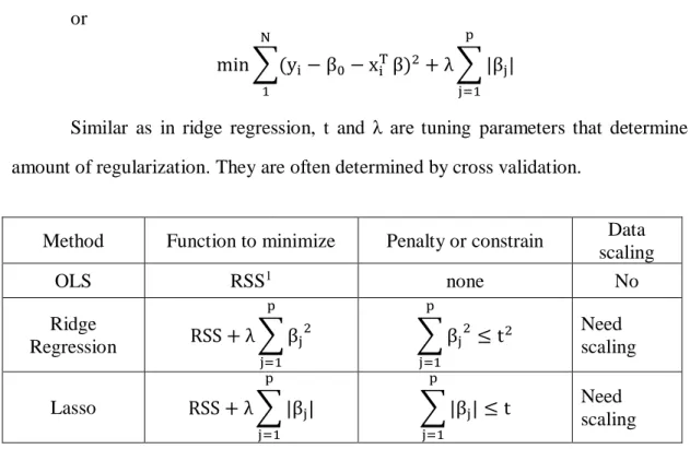
Similar as in ridge regression, t and λ are tuning parameters that determine the amount of regularization. They are often determined by cross validation.

Method Function to minimize Penalty or constrain Data scaling OLS RSS1 _none _No Ridge Regression RSS + λ ∑ βj 2 p j=1 ∑ βj2 ≤ t2 p j=1 Need scaling Lasso RSS + λ ∑ |β_j| p j=1 ∑ |β_j| ≤ t p j=1 Need scaling

Table 4.1: Comparison of OLS regression Ridge regression and Lasso Regression

The most important idea of Ridge regression and Lasso regression is shrinkage, which impose a penalty (constraint) in the objective function so that the size of the coefficients can be controlled. Shrinkage will help the training model fit not only the training data, but also the test data, which is a big issue of OLS regression with datasets with a large set of predictors. However, the potential risk is that the shrinkage process produces biased results although the variance is reduced. Unlike OLS, the coefficient of Ridge regression and Lasso regression can change with scaling. Thus, it’s important to scale the data before doing Ridge or Lasso regression.

(18)

4.2TREE BASED MODEL

Tree based methods empower predictive models with high accuracy and stability. Unlike regression based models that only can do linear relationships, tree base models can map both linear and non-linear relationships quite well. In this work we use Random Forest model and Gradient Boosted Machines which are considered to be two of the mostly used tree based learning algorithms.

4.2.1 Random forest model

Random forest or random decision forest is a versatile machine learning method for clustering, classification, regression. It can also be applied in situations that many other algorithms are unable to apply, for example, when the dataset has a large dimension, contains large number of missing values or number of outlier values [7].

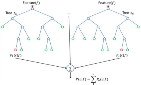
Figure 4.1: The process of Random Forest

The original algorithm of random tree was developed by Leo Breiman and Adele Cutler. The term of random decision forests was first proposed by Tin Kam Ho of Bell

(19)

Labs in 1995. By constructing a multitude of decision trees at training, a random forest model outputs a class that is the mode of the classes or the mean of predictions of the individual trees. The process is shown in Figure 4.1. The meta-algorithm of random forest is Bagging, which stands for Bootstrap Aggregating. Tt is a way to decrease the prediction variance by creating additional data for training which resamples from the original dataset [7].

4.2.2 GBM model

Gradient boosting machine or generalized boosted model (GBM) is a machine learning technique for regression and classification problems. This method builds a prediction model also in the form of decision trees [10]. The meta algorithm of GBM is boosting. The boosting process is a two-step approach. The first step is using subsets of the original data to produce a series of averagely performing models. The second step is "boost" the performance of models produced in the first step by combining them together and using an arbitrary differentiable loss function. The objective of GBM is minimizing the exponential loss function which can be expressed as following:

Loss = ∑ exp(−1 2yi ∑ am M m=1 Gm(xi N 1 ))

Here G is the classifier with possible values 1 or -1. The GBM model applies several hyper parameters in order to determine the most optimal model. The first parameter is number of trees which indicating the terminal nodes in trees. The second parameter is called regularization parameter.One regularization parameter is the number of gradient boosting iterations. Increasing iteration will reduce the error of the training model, but if the number of iterations is too high, it may cause the problem of overfitting.

(20)

method. It is regularization by shrinkage which consists in modifying the update rule. Empirical findings show that smaller learning rates will improve model generalization. The fourth parameter is maximum depth which specifies the maximum depth to which each tree will be built [10].

4.2.3 Comparison of Random forest and GBM

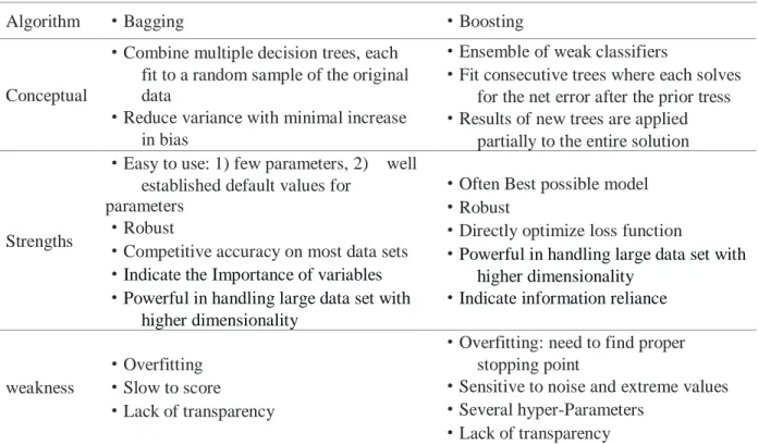
Both Random forest model and GBM model are ensemble methods, which build a classifier out of a big number of smaller classifiers. There are several differences between the two methods, which are indicated in Table (4.2).

Random forest GBM

Algorithm ·Bagging ·Boosting

Conceptual

·Combine multiple decision trees, each fit to a random sample of the original data

·Reduce variance with minimal increase in bias

·Ensemble of weak classifiers

·Fit consecutive trees where each solves for the net error after the prior tress

·Results of new trees are applied partially to the entire solution

Strengths

·Easy to use: 1) few parameters, 2) well established default values for

parameters

·Robust

·Competitive accuracy on most data sets

·Indicate the Importance of variables

·Powerful in handling large data set with higher dimensionality

·Often Best possible model

·Robust

·Directly optimize loss function

·Powerful in handling large data set with higher dimensionality

·Indicate information reliance

weakness

·Overfitting

·Slow to score

·Lack of transparency

·Overfitting: need to find proper stopping point

·Sensitive to noise and extreme values

·Several hyper-Parameters

·Lack of transparency

(21)

The fundamental difference between Random forest and GBM lies on their mega-algorithms. Random forest model grows trees in parallel. This process has low bias but high variance. Random forest is based on the algorithm of bagging which resamples the data for many times. By making uncorrelated trees, this process can maximize the decline of variance but minimal the increase of bias [8].

(22)

Chapter 5: Application of Machine Learning

in Material Property Prediction

Transparent conductors are an important class of compounds that are both electrically conductive and have a low absorption in the visible range. A combination characteristic of electrical conductive and low absorption is the key for the operation of a variety of technological devices such as photovoltaic cells, light-emitting diodes for flat-panel displays, transistors, sensors, touch screens, and lasers. However, only very small number of compounds which display both transparency and conductivity are suitable enough to be used as transparent conducting materials [12].

In this work we develop machine learning models to predict the two important physically-distinct properties of transparent conductors: the band gap energy and formation enthalpy.

5.1DATA AND VARIABLE DESCRIPTIONS

The original data is from an open big-data competition which was organized by Novel Materials Discovery Repository (NOMAD) and Kaggle for the prediction both the formation enthalpy and the bandgap energy [18]. In the data set there are 2400 observations of 13 variables, and it includes the following information: 1) space group , 2) total number of Al, Ga, In and O atoms in the unit cell, 3) relative compositions of Al, Ga, and In, 4)Lattice vectors and angles: lv1, lv2, lv3, which are lengths given in units of angstroms (unit: 10−10 meters) and α, β, γ, which are angles in degrees between 0° and 360°. We develop models to predict the two physically-distinct properties: i) formation enthalpy which is an indication of the stability of a new material and ii) the bandgap energy which is an indication of the potential for transparency over the visible range.

(23)

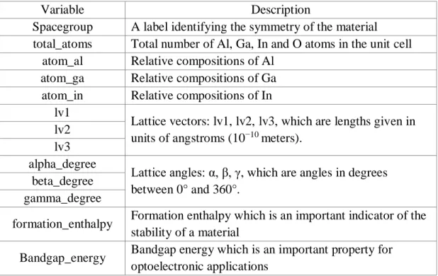
Table 5.1: Variable description

5.2DATA EXPLORATION AND VISUALIZATION

Table 5.2 and Table 5.3 show a statistical summary of numeric variables and categorical variables. Based on the skewness and kurtosis value, the distribution of observed values of formation enthalpy and bandgap energy are not symmetric or normal.

Variable Description

Spacegroup A label identifying the symmetry of the material total_atoms Total number of Al, Ga, In and O atoms in the unit cell

atom_al Relative compositions of Al atom_ga Relative compositions of Ga atom_in Relative compositions of In

lv1

Lattice vectors: lv1, lv2, lv3, which are lengths given in units of angstroms (10−10 meters).

lv2 lv3 alpha_degree

Lattice angles: α, β, γ, which are angles in degrees between 0° and 360°.

beta_degree gamma_degree

formation_enthalpy Formation enthalpy which is an important indicator of the stability of a material

Bandgap_energy Bandgap energy which is an important property for optoelectronic applications

(24)

Table 5.2: Statistical summary of numeric variables

From Table 5.3 we can see that based on the categorical variable “spacegroup” the observations are almost balanced; however, based on the categorical variable “total atoms”, the data set is unbalanced.

spacegroup 12 33 167 194 206 227

Frequency 11.93% 14.44% 12.46% 11.76% 16.33% 13.10%

total atoms 10 20 30 40 60 80

Frequency 0.43% 2.80% 10.87% 17.30% 1.60% 47.00%

Table 5.3: Statistical Summary of Categorical variables

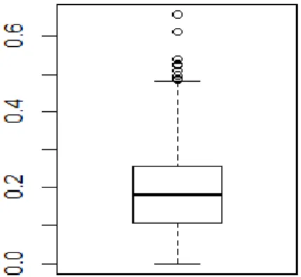
We also created histograms and boxplots to assess the distribution of the response variables of formation enthalpy and bandgap energy, so that we can have a more intuitive picture of their distribution.

Variable mean min Max Standard

deviation skew kurt

atom_al 0.385 1 0 0.266 0.175 2.115 atom_ga 0.308 1 0 0.236 0.546 2.541 atom_in 0.306 1 0 0.2631 0.681 2.589 lv1 10.030 24.913 3.037 5.645 1.748 5.137 lv2 7.087 10.290 2.942 1.890 0.064 1.943 lv3 12.5 25.346 5.673 5.450 1.054 3.252 alpha_degree 90.244 101.230 82.744 1.334 4.036 29.931 beta_degree 92.398 106.168 81.641 5.299 1.746 4.341 gamma_degree 94.787 120.054 29.727 25.868 -1.248 4.261 formation_enthalpy 0.187 0.6572 0.104 0.104 0.465 2.779 Bandgap_energy 2.077 5.2861 0 0.100 0.559 2.658

(25)

Figure 5.1: Distribution of formation enthalpy

From the histogram and boxplot (Figure 5.1) of formation enthalpy, the distribution of formation is not normal and displays a right skewed shape. And there are several outliers showing in the boxplot.

(26)

From the histogram and boxplot (Figure 5.2) of bandgap energy, the distribution of bandgap energy is not normal and also displays a right skewed shape. And there are several outliers showing in the boxplot.

Figure 5.3: Scatter plots of formation enthalpy

Figure 5.3 and Figure 5.4 are paired scatter plots of response variable and each numeric categorical variable. Based on Figure 5.3, only the explanatory variable percent of atom ga shows an approximately negative linear relationship with the response variable formation enthalpy.

(27)

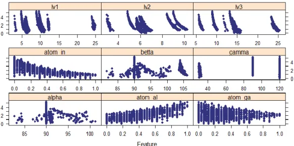
Figure 5.4: Scatter plots of bandgap energy

According to the paired scatter plot of bandgap energy (Figure 5.4), there is a negative linear relationship between percentage of atom in and bandgap energy and a positive linear relationship between percentage of atom al and bandgap energy. The percentage of atom ga has a negative correlation to bandgap energy.

(28)

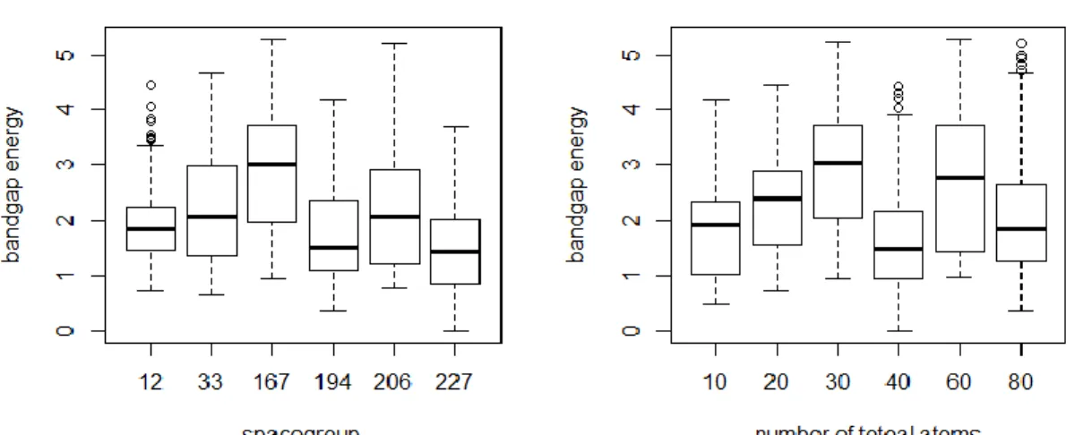
Figure 5.6: Boxplot of bandgap energy with different categorical variables

Figures 5.5 and 5.6 are group boxplots for the description of bivariate relationship between categorical explanatory variables and response variable. According to the group boxplots of formation enthalpy (Figure 5.5), we can find that the median values of formation enthalpy vary much with different categories. The space group 227 and number of total atoms 40 has the largest median values of formation enthalpy, and the space group 194 and the number of total atoms 80 has most outlier among different categories, respectively.

According to Figure 5.6, we can find that the space group 167 and number of total atoms 40 has the largest media values of bandgap energy, and the space group12 and the number of total atoms 80 has most outlier among different categories respectively. 5.3SAMPLE PREPARATION

First, we have to detect Zero-variance predictors. The result shows that none of the 11 predictors in our dataset have zero-variance. Therefore, no predictor variables need be eliminated before developing the model.

(29)

Second, we have to identify Correlated Predictors. In our original data set, among the 11 predictors, 9 of them are numeric variables. We suspect that there might be some of the features that are linearly correlated with each other.

Figure 5.7: Correlation matrix of the numeric predictors

To determine collinearity in our data, we visualized the correlation matrix of the numeric predictors (Figure 5.7). If a pair of features are highly correlated with each other, the correlation will exhibit as a dark blue (positive correlated) or dark red (negative correlated) dot. Based on the above graph, there is no highly correlated predictors (r > ± 0.85) in the data set.

Third, variable transformation is needed. According to the statistical summary and the distribution graphs (histogram and boxplot), the distribution of response variables,

(30)

conduct a log transformation of the two variables. Moreover, since some observed values of formation enthalpy and bandgap energy are zero or very close to zero, we need to add one to the original value before transformation, as the following:

𝑦_𝑛𝑒𝑤 = 𝑙𝑜𝑔 (𝑦_𝑜𝑟𝑖𝑔𝑖𝑛𝑎𝑙 + 1)

Here y_original is the observed value of formation enthalpy or bandgap energy in the original data set, y_new is the transformed value which will be used in model training. 5.4FORMATION ENTHALPY PREDICTION

5.4.1 Regression based Models

In this part we develop four regression based models to predict the formation enthalpy, including OLS regression model, forward selection model, Ridge regression model and Lasso regression model.

Variable Estimate Std.Error t statistic p-value

Intercept 0.16837 0.0016 99.540 0<2e-16 *** Spacegroup 0.0047 0.0025 1.884 0.05971 * total_atoms -0.0159 0.0065 -2.412 0.01597 ** atom_al 27.5505 10.8314 2.544 0.01107 ** atom_ga 24.2189 9.5323 2.541 0.01116 ** atom_in 27.3130 10.7347 2.544 0.01104 ** lv1 0.0208 0.0076 2.717 0.00666 *** lv2 0.0078 0.0066 1.179 0.23868 lv3 0.0535 0.0048 10.945 <2e -16 *** alpha_degree -0.0053 0.0025 -2.073 0.03831 ** beta_degree -0.0043 0.0057 -0.756 0.44958 gamma_degree -0.0147 0.0028 -5.133 3.2 e-07 *** ***, **, * indicate rejection of the null hypothesis at the 1%, 5%, 10% levels of significance Table 5.4: OLS model for formation enthalpy

(31)

According to the result shown in Table 5.4, OLS model includes all the 11 predictors in the model and no interaction between explanatory variables is considered. The residual standard error is 0.0672 on 1573 degree of freedom. And the Adjusted R-squared is 0.391, which means the OLS model explained 39.1% of the variance of the response variable. Among the 11 explanatory variables 9 of them are at least 10% significant, while lv2 and beta degree are not significant which have regression coefficient equal to 0.0078and -0.0043 respectively.

Variable Estimate Std.Error t statistic p-value

intercept 0.168384 0.0017 99.570 <2e -16 *** spacegroup 0.00535 0.0023 2.274 0.02311 ** total_atoms -0.0156 0.0065 -2.372 0.01779 ** atom_al 27.4888 10.8296 2.538 0.01124 ** atom_ga 24.1645 9.5307 2.535 0.01133 ** atom_in 27.2517 10.7330 2.539 0.01121 ** lv1 0.0175 0.0063 2.792 0.00529 *** lv2 0.0091 0.0064 1.419 0.15612 lv3 0.0538 0.0048 11.069 <2e -16 *** alpha_degree -0.0062 0.0022 -2.830 0.00472 *** gamma_degree -0.0152 0.0027 -5.497 4.5 e-08 *** ***, **, * indicate rejection of the null hypothesis at the 1%, 5%, 10% levels of significance Table 5.5: Forward selection regression for formation enthalpy

According to the result of OLS model, we find that the OLS regression process will include all explanatory variables in the model including those insignificant ones. Thus, we try the stepwise selection model to build a regression model from the 11 candidate predictor variables by entering predictors based on p-values of the F-test in a forward stepwise manner until there is no variable left to enter. The result shows as in Table 5.5 that 10 predictors entered the model. The one factor with a beta degree not

(32)

The residual standard error of forward selection model is 0.0672 with 1573 degrees of freedom and the adjusted R-squared is 0.391. These two values are the same as OLS model, which means the variable "beta degree" does not explain extra information in OLS model.

By adding a penalty term in the objective model (for ridge model the penalty is the sum of squares of the regression coefficients, for lasso model the penalty is the sum of absolute values of the regression coefficients), we also develop Ridge regression model and Lasso regression model to predict the formation enthalpy. By 10-folds cross validation, the tuning parameter λ of Ridge and Lasso were found to be 0.00435 and 0.00003 respectively. In Ridge model all the 11 explanatory variables are included, and in Lasso model there are 10 explanatory variables, while atom_al is removed.

Varable OLS Forward selection Ridge Lasso

intercept 0.16836 0.16838 0.16841 0.16840 spacegroup 0.0047 0.00535 0.0062 0.0049 total_atoms -0.0159 -0.0156 -0.0007 -0.0141 atom_al 27.5505 27.4888 0.0039 --- atom_ga 24.2189 24.1645 -0.0219 -0.0272 atom_in 27.3130 27.2517 0.0154 0.0087 lv1 0.0208 0.0175 0.0053 0.0188 lv2 0.0078 0.0091 -0.0060 0.0062 lv3 0.0535 0.0538 0.0394 0.0521 alpha_degree -0.0053 -0.0062 -0.0039 -0.0052 beta_degree -0.0043 --- -0.0031 -0.0038 gamma_degree -0.0147 -0.0152 -0.0161 -0.0151

Table 5.6: Coefficients of the regression based models for formation enthalpy Table 5.6 shows the comparison of the regression coefficients of the four

(33)

coefficients (except variable "spacegroup") of the Ridge model and the Lasso model are much smaller than that in the OLS model and forward selection models. However, since the train dataset does not have large number of predictors and there is no significant multicollinearity among these predictors, the advantage of ridge regression model in addressing the collinearity and lasso regression model in selecting effective predictors are not obvious in this work.

5.4.2 Tree based models

Random forest and GBM are two improved decision tree models. In this work we develop random forest model, GBM model, random forest model with parameter tuning, and GBM with parameter tuning to predict the formation enthalpy.

(1) Random forest and GBM

In the Random forest model, 500 decision trees are built and 3 explanatory variables are tried at each split of decision tree. The mean of squared residuals is 0.0011, which is much lower than linear regression based models. And the model explained 84.64% variance of the response variable which is much higher than OLS model and forward selection model.

For the GBM model, the optimal number of trees is 3530 which is tuned by using 3-folds cross validation with a learning rate of 0.05. The squared residual of the GBM model is 0.00075 which is smaller than Random forest model.

For random forest model, the variable importance is measured by the %IncMSE2 and IncNodePurity3, for GBM model, the variable importance is measured by the relative

(34)

influence in percentage. According to the results in Table 11, for random forest the 3 most important predictors are atom_in, altom_al and atom_ga. For GBM, the 3 most important predictors are lv3, atom_in and alpha degree.

variable

Random forest GBM

%IncMSE Rank IncNodePurity

%Relative influence Rank spacegroup 28.2820 7 0.8278 2.3022 9 total_atoms 13.1580 10 0.0928 0.1351 10 atom_al 46.3496 2 0.7856 7.2612 5 atom_ga 37.5748 3 0.8393 4.6781 7 atom_in 60.0350 1 2.0000 17.6007 2 lv1 25.2294 8 0.6989 2.3788 8 lv2 35.4440 4 1.0261 5.4977 6 lv3 32.0349 5 2.2798 31.6058 1 alpha_degree 27.5459 8 1.6733 16.2490 3 beta_degree 30.9049 6 0.5856 8.8788 4 Gamma_degree 18.8619 10 0.5044 3.4122 7

Table 5.7: Variable importance of Random forest and GBM (2) Random forest and GBM with tuning

In order to enhance the predicting performance of Random forest model and GBM model, we can tune the critical parameters of the two models.

For Random forest model, three primary features can be tuned to improve the predictive power. 1) m-try. This is the maximum number of features that Random forest allowed to try in individual tree (this number cannot exceed the total number of predictors). Increasing max features generally improves the performance of the model. However, it will decrease the speed of model and increase computation cost. 2) n-tree. This is the number of trees you want to build before taking the maximum voting or

(35)

averages of predictions. Usually, the larger the number of the trees the better performance you will get. But increasing the number of trees will make the process slower. 3) node-size. Node size is the number of nodes in the end node of a decision tree. A smaller node size makes the model more prone to capturing noise in training data, but it may cause the problem of overfitting.

Here we create a gird with m-try equal to a sequence from 1 to 10 and each time increase by 1, n-tree equal to 500 and 1000, and node-size equal to 1, 5, 25 and 50. Thus 80 random models are built, and we pick up the best model with least train RMSE 0.03350 to predict the formation enthalpy in test data.

For GBM model, the parameters for managing boosting are described below. 1) Shrinkage also called as learning-rate determines the impact of each tree on the final outcome. Lower values are generally preferred as they make the model more robust. However, Lower values would require higher number of trees to model all the relations and will be computationally expensive. 2) The parameter n-trees is the number of sequential trees to be modeled. The optimal number of trees should be tuned by using CV with a particular learning rate. 3) Bag-fraction is the fraction of observations to be selected for each tree which is done by random sampling. 4) Interaction-depth is a number of splits that the process has to perform on a tree (starting from a single node).

The girds to tune parameters for the GBM model described in the following. N-trees are from 200 to 2000 and each time increases by 400. The shrinkage is equal to 0.001, 0.05 and 1. The bag-fraction is equal to 0.5 and1. The interaction-depth is from 6 to 8, and each time increase by 1. Thus 90 GBM models are built and we will pick the optimal model with the smallest training RMSE which is 0.003305 to predict the

(36)

5.4.3 Model evaluation and comparison

To check the validation of the eight models, we made QQ plots of residuals (Figure 5.8 and Figure 5.9) and scatter plots of fitted value and observed value in test dataset (Figure 5.10).

Figure 5.8: QQ plots of regression based Models for formation enthalpy

According to the QQ plots we can see that for the four regression based models, the theoretical quantiles and sample quantiles fit a linear relationship very well, which means the distribution of residuals are normal. Because all the four models meet the assumption of Multivariate normality, they are valid in some extend.

(37)

Figure 5.9: QQ plots of tree based models for formation enthalpy

According to the QQ plots of the tree based model (Figure5.9), we can see that the theoretical quantiles and sample quantiles of the four models do not fit a linear relationship, which means the residuals of the four models are not normally distributed. Since tree based models are not based on the basic assumptions of normality like regression based model, thus we cannot evaluate tree based model according to the QQ plots.

(38)

Figure 5.10: Scatter lot of predict values vs observed values of formation enthalpy We compare the predictive performance of the eight models by plotting scatter plots with the predicted values and the observed the values of the formation enthalpy of the test dataset, and also by drawing a red line with an intercept of zero and slope of 1. If the model is a “perfect” predictive model, a plot of the predictions versus observed values would match exactly and the points will cluster around the red line. Depending on the scatter plots (Figure 5.10), we can find that the four tree based models perform much

(39)

better than the regression based models in predicting response variable. However, depending on these graph it is difficult to evaluate the performance among the four regression based models and the performance among the four tree based models. Therefore, we calculate the train RMSE and test RMSE of each model to compare their predictive performances. Since RMSE is an error metric, the lower the values, the better predictive performance is.

Regression based

model OLS Forward Ridge Lasso

Train RMSE 0.06694 0.06695 0.06888 0.06831

Test RMSE 0.06824 0.06828 0.06986 0.06940

Tree based model Random forest

Random Forest

(tuning) GBM GBM(tuning)

Train RMSE 0.01983 0.03350 0.02881 0.03305

Test RMSE 0.03547 0.03552 0.03699 0.03346

Table 5.8: RMSE of the four models for formation enthalpy

The train RMSE and test RMSE of formation enthalpy are recorded in Table 5.8. The train RMSE for regression based models are 0.06694 for OLS model, 0.06695 for forward selection model, 0.06888 for ridge model, and 0.06831 for Lasso model. In contrast, their test RMSE are 0.06824 for OLS model, 0.06828 for forward selection model, 0.06986 for ridge model, and 0.06940 for Lasso model. The train RMSE of bandgap energy for tree based models are 0.01983 for Random forest model, 0.0350 for Random forest model with tuning, 0.02881 for GBM model, and 0.03305 for GBM model with tuning. Accordingly, their test RMSE are 0.03547, 0.03552, 0.03699, and 0.03346 respectively.

(40)

It is obvious that the tree based models have better performance than regression based models since the average test RMSE of tree base models are much smaller than regression based models. Among the four regression based models, OLS model has the smallest Train RMSE and test RMSE. Besides, the test RMSE of regression based models are close to their train RMSE respectively, so there is no problem of overfitting for regression based models. For the four tree based models, based on the train RMSE and test RMSE, GBM with tuning is the best model. Although the Random forest model and GBM model with no tuning have relatively smaller train RMSE, their difference between train RMSE and test RMSE are larger. Thus, there is a problem of overfitting in Random forest and GBM.

5.5BANDGAP ENERGY PREDICTION

In this part we develop four regression based models including OLS, Forward selection model, Ridge regression and Lasso regression model, as well as four tree based models including Random forest, random forest with tuning, GBM and GBM with tuning to predict the bandgap energy.

OLS model includes all the 11 predictor variables, 8 of which are at least 10% significant, while 3 of them (atom_al, atom_ga, atom_in) are not significant. The Residual standard error of OLS is 0.1473 on 1573 degrees of freedom and the adjusted R-squared is 0.8024, which means the model explained 80.24% variance of the response variable.

The forward selection model has 10 predictors (the variable atom_in is removed), and all the 10 predictors are at least 10% significant. The Residual standard error is 0.1473 on 1573 degrees of freedom. The adjusted R-squared is 0.8025 which is very close to the adjusted R-squared of OLS model.

(41)

By 10-folds cross validation, the tuning parameter λ of Ridge model and Lasso mode were found to be 0.02816 and 0.00015, respectively. In Ridge model all the 11 explanatory variables are included, and in Lasso model there are 10 explanatory variables, while atom_ga is removed.

According to the regression coefficients in Table 5.9, after controlling the size of the coefficients using penalty terms, the regression coefficients of Ridge model and Lasso model are much smaller than that in OLS model and forward selection models.

Variable OLS Forward selection Ridge Lasso

intercept 31.020 0.91790** 0.57304 0.44141 spacegroup -0.00024*** -0.00021*** -0.00024 -0.00021 total_atoms 0.00538*** 0.00538*** 0.00098 0.0049 Atom_al -30.11 -0.4601*** 0.52313 0.46276 atom_ga -30.57 -1.078*** 005460 --- atom_in -31.18 -- -0.58959 -0.62361 lv1 -0.02199*** -0.02199*** -0.00661 -0.02077 lv2 -0.05342*** -0.05343*** -0.00372 -0.04867 lv3 -0.03330*** -0.03330*** -0.01800 -0.03214 alpha_degree 0.01910*** 0.01911*** 0.01049 0.01847 beta_degree -0.00587* -0.00587* -0.00423 -0.00554 gamma_degree 0.00168*** 0.00168*** 0.00207 0.00174 ***, **, * indicate rejection of the null hypothesis at the 1%, 5%, 10% levels of significance Table 5.9: Coefficients of regression based models4

In the Random forest model, 500 decision trees are built, and 3 explanatory variables are tried at each split of decision tree. The mean of squared residuals is 0.0086, which is much lower than regression based models. And the model explained 92.15% variance of the response variable which is much higher than OLS model or forward selection model.

(42)

The tuning parameters for the random forest model are: m-try equal to a sequence from 1 to 10 and each time increase by 1, n-tree equal to 500 and 1000, and node-size equal to 1, 5, 25 and 50. Thus 80 random models are built, and the best model has m-try equals to 2, n-tree equals to 1000, node-size equals to 1. The train RMSE of the tuned model is 0.09409 which is higher than Random forest model without tuning.

In the GBM model, the optimal number of trees is 1433 which is tuned by using 3-folds cross validation with a learning rate of 0.05. The squared residual of the GBM model is 0.00485 which is smaller than Random forest model.

The tuning parameters for the GBM model are: n-trees is from 200 to 2000 and each time increase by 400, the shrinkage are equal to 0.001, 0.05 and 1, the bag-fraction is equal to 0.5 and1, while interaction-depth is from 6 to 8, and each time increase by 1. Among the 90 GBM models, the optimal model has an interactiodepth equals to 7, n-trees equals to 200, shrinkage is 0.05 and the bag-fraction is 0.5. The train RMSE of the optimal GBM model is 0.09173.

(43)

Figure 5.11: QQ plots of residuals for regression based models

According to the QQ plots (Figure 5.12) we can see that the theoretical quantiles and sample quantiles for the four regression based models do not fit a linear relationship, which means the basic assumption of multivariate normality is not met. Because the observed data of bandgap energy is not approximately normal even after the log transformation, thus the regression based models do not do a good job in predicting bandgap energy.

(44)

Figure 5.12: Scatter plots of predict values VS observed values of bandgap energy Depending on the scatter plots (Figure 5.13) of fitted value and observed values of bandgap energy in test data set we can see that the four tree based models perform much better than the regression based models in predicting response variable. We also calculate the train RMSE and test RMSE of each model to compare their predictive performance more precisely.

Regression based model

OLS Forward Ridge Lasso

Train RMSE 0.14026 0.14033 0.14947 0.14623

Test RMSE 0.14567 0.14568 0.15506 0.15230

Tree based

model Random forest

Random Forest

(tuning) GBM GBM(tuning)

Train RMSE 0.04991 0.09409 0.07841 0.09173

Test RMSE 0.09252 0.09274 0.09261 0.09210

Table 5.10: The RMSE of the eight models for bandgap energy

The train RMSE and test RMSE of bandgap energy are recorded in Table 5.10. The train RMSE for regression based models are 0.14026 for OLS model, 0.14033 for forward selection model, 0.14947 for ridge model, and 0.14623 for lasso model, while their test RMSE are 0.14567 for OLS model, 0.14568 for forward selection model, 0.15506 for ridge model, and 0.15230 for lasso model. The train RMSE of bandgap energy for tree based models are 0.04991 for Random forest model, 0.09409 for Random forest model with tuning, 0.0781 for GBM model, and 0.09173 for GBM model with tuning; accordingly, their test RMSE are 0.09252, 0.09274, 0.09261, and 0.09210 respectively.

(45)

Based on RMSE in Table 5.10, the performance of tree based model are much better than regression based models. OLS model has the smallest train RMSE and test RMSE among the four regression based models. And there is no problem of overfitting for the four regression based models, because the test RMSE of each model is close to their train RMSE respectively. GBM with tuning is the best model among the four tree based models because it has the smallest test RMSE. Although the Random forest model and GBM model have relatively smaller train RMSE, their difference between train RMSE and test RMSE are larger. Thus there is a problem of overfitting in these two models.

(46)

Chapter 6: Conclusions and Future Work

In this report, we built four regression based models and four tree based models with the train dataset to predict formation enthalpy and bandgap energy which are two critical properties of transparent conductors. The regression based models include OLS regression model, Stepwise selection model, Ridge model and Lasso model. The tree based models include random forest model, random forest model with tuning, GBM model and GBM model with tuning.

In order to compare the model performance in predicting materials properties, we used root mean square error (RMSE) as an evaluation metric. Based on the train RMSE and test RMSE, the conclusions of model performance are consistence for formation enthalpy and bandgap energy.

First, the performances of tree based models are much better than regression based models. For formation enthalpy, the average test RMSE of tree based models is 0.03536, while the average test RMSE of regression based model is 0.06894. For bandgap energy, the average test RMSE of tree based models is 0.09249, while the average test RMSE of regression based model is 0.14961.

Second, among the four regression based models, OLS model has the smallest train RMSE and test RMSE. There is no problem of overfitting in the four regression based models since the difference between train RMSE and test RMSE of each model is small. The advantages of Ridge model and lasso model in dealing with multicollinearity and overfitting are not obvious, because our original dataset does not have a large number predictor and no significant collinearity among the eight numerical explanatory variables. Moreover, among the four tree based models, the Random forest model has the smallest train RMSE, but has the second largest test RMSE, which reflect a problem of

(47)

overfitting. Similar as the Random forest model, the GBM model also over fits the train data, since it has the second smallest train RMSE while has the largest test RMSE. Tuning critical parameters can significantly improve the problem of overfitting, since the differences between the train RMSE and the test RMSE are greatly reduced after tuning. Finally, among the eight models, GBM with tuning has the smallest train RMSE and smallest difference between the train RMSE and the test RMSE. Therefore, GBM with tuning has significant advantage over regression based machine learning and statistical analysis tools such as multivariate regression models, Ridge model and Lasso models and also other three tree based models. And it selects predictors with greater stability and transferability, with a goal to understand the inner mechanism rather than over-fitting data.

Although we have covered several machine learning models in this report, these are simple models not considering higher order effects such as interaction and squared and cubic terms. There are still many more models left to be explored, for example, Support Vector Regression, Artificial Neutral Network, K-nearest Neighbor, Extreme Gradient Boosting. These models are all models which worth trying in the future.

(48)

References

1. A. Agrawal and A. Choudhary, International Journal of Fatigue, 113 (2018). An online tool for predicting fatigue strength of steel alloys based on ensemble data mining. 2. A. Paul, P. Acar, R. Liu, American Institute of Aeronautics and Astronautics (AIAA)

Journal, 3, 56 (2018), Data Sampling Schemes for Microstructure Design with

Vibrational Tuning Constraints.

3. R. LeSar, Stat. Anal. Data Min., 1, 372 (2009). Materials Informatics: An Emerging Technology for Materials Development.

4. K. Rajan, Mater. Today, 8, 38 (2005). Materials Informatics.

5. G. Hautier, C. C. Fischer, A. Jain, T. Mueller, and G. Ceder, Chem. Mater., 22, 3762 (2010). Finding Nature’s Missing Ternary Oxide Compounds Using Machine Learning and Density Functional Theory.

6. G. Pilania, C. Wang, X. Jiang, S. Rajasekaran, and R. Ramprasad, Sci. Rep., 3, 1 (2013). Accelerating Materials Property Predictions Using Machine Learning.

7. H Tin Kam, IEEE Transactions on Pattern Analysis and Machine Intelligence, 8, 20 (1998). The Random Subspace Method for Constructing Decision Forests.

8. K. Hansen, G. Montavon, F. Biegler, S. Fazli, M. Rupp, M. Scheffler, O. A. von Lilienfeld, A. Tkatchenko, and K.‐R. Müller, J. Chem. Theory Comput., 9, 3404 (2013). Assessment and Validation of Machine Learning Methods for Predicting Molecular Atomization Energies.

9. K. Hansen, F. Biegler, R. Ramakrishnan, etc, J. Phys. Chem. Lett., 6, 2326 (2015). Machine Learning Predictions of Molecular Properties: Accurate Many‐Body Potentials and Nonlocality in Chemical Space.

10. J. H. Friedman, (February 1999), Greedy Function Approximation: A Gradient Boosting Machine.

11. L. Ruoqian, K. Abhishek, C. Zhengzhang, scientific reports, 10, (2015). A predictive machine learning approach for microstructure optimization and materials design.

(49)

12. M. Tim, G. K. Aaron, Reviews in Computational Chemistry, 29, (2016). Machine learning in materials science: recent progress and emerging applications.

13. R. Pelánek, User Modeling and User-Adapted Interaction, (2017), Bayesian Knowledge Tracing, Logistic Models, and Beyond: An Overview of Learner Modeling Techniques.

14. V. Botu and R. Ramprasad, Phys. Rev. B, 92, 094306 (2015). Learning Scheme to Predict Atomic Forces and Accelerate Materials Simulations.

15. R. Tibshirani, J. R. Stat. Soc. Ser. B Methodol., 58, 267 (1996). Regression Shrinkage and Selection via the Lasso.

16. B. Efron and G. Gong, Am. Stat., 37, 36 (1983). A Leisurely Look at the Bootstrap, the Jackknife, and Cross‐Validation.

17. S. Arlot and A. Celisse, Stat. Surv., 4, 40 (2010). A Survey of Cross‐Validation Procedures for Model Selection.

18. The dataset is from https://www.kaggle.com/c/nomad2018-predict-transparent-conductors